| Issue |
A&A
Volume 639, July 2020
|
|
|---|---|---|
| Article Number | A57 | |
| Number of page(s) | 13 | |
| Section | Cosmology (including clusters of galaxies) | |
| DOI | https://doi.org/10.1051/0004-6361/201936720 | |
| Published online | 07 July 2020 | |
Cosmic dissonance: are new physics or systematics behind a short sound horizon?
1
DARK, Niels-Bohr Institute, Lyngbyvej 2, 2100 Copenhagen, Denmark
e-mail: This email address is being protected from spambots. You need JavaScript enabled to view it.
2
Physics Department UC Davis, 1 Shields Ave., Davis, CA 95616, USA
3
STAR Institute, Quartier Agora – Allée du six Août, 19c B-4000 Liège, Belgium
4
Exzellenzcluster Universe, Boltzmannstr. 2, 85748 Garching, Germany
5
Ludwig-Maximilians-Universität, Universitäts-Sternwarte, Scheinerstr. 1, 81679 München, Germany
6
Laboratoire d’Astrophysique, École Politechnique Fédérale de Lausanne (EPFL), Obs. de Sauverny, 1290 Versoix, Switzerland
7
Kavli IPMU (WPI), UTIAS, The University of Tokyo, Kashiwa, Chiba 277-8583, Japan
8
Max-Planck-Institut für Astrophysik, Karl-Schwarzschild-Str. 1, 85748 Garching, Germany
9
Physik-Department, Technische Universität München, James-Franck-Straße 1, 85748 Garching, Germany
10
Academia Sinica Institute of Astronomy and Astrophysics (ASIAA), 11F of ASMAB, No.1, Sect. 4, Roosevelt Rd, Taipei 10617, Taiwan
11
Department of Physics and Astronomy, University of California, Los Angeles, CA 90095, USA
12
Kavli Institute for Particle Astrophysics and Cosmology and Department of Physics, Stanford University, Stanford, CA 94305, USA
13
Kapteyn Astronomical Institute, University of Groningen, PO Box 800, 9700 AV Groningen, The Netherlands
Received:
17
September
2019
Accepted:
7
May
2020
Abstract
Context. Persistent tension between low-redshift observations and the cosmic microwave background radiation (CMB), in terms of two fundamental distance scales set by the sound horizon rd and the Hubble constant H0, suggests new physics beyond the Standard Model, departures from concordance cosmology, or residual systematics.
Aims. The role of different probe combinations must be assessed, as well as of different physical models that can alter the expansion history of the Universe and the inferred cosmological parameters.
Methods. We examined recently updated distance calibrations from Cepheids, gravitational lensing time-delay observations, and the tip of the red giant branch. Calibrating the baryon acoustic oscillations and type Ia supernovae with combinations of the distance indicators, we obtained a joint and self-consistent measurement of H0 and rd at low redshift, independent of cosmological models and CMB inference. In an attempt to alleviate the tension between late-time and CMB-based measurements, we considered four extensions of the standard ΛCDM model.
Results. The sound horizon from our different measurements is rd = (137 ± 3stat. ± 2syst.) Mpc based on absolute distance calibration from gravitational lensing and the cosmic distance ladder. Depending on the adopted distance indicators, the combined tension in H0 and rd ranges between 2.3 and 5.1 σ, and it is independent of changes to the low-redshift expansion history. We find that modifications of ΛCDM that change the physics after recombination fail to provide a solution to the problem, for the reason that they only resolve the tension in H0, while the tension in rd remains unchanged. Pre-recombination extensions (with early dark energy or the effective number of neutrinos Neff = 3.24 ± 0.16) are allowed by the data, unless the calibration from Cepheids is included.
Conclusions. Results from time-delay lenses are consistent with those from distance-ladder calibrations and point to a discrepancy between absolute distance scales measured from the CMB (assuming the standard cosmological model) and late-time observations. New proposals to resolve this tension should be examined with respect to reconciling not only the Hubble constant but also the sound horizon derived from the CMB and other cosmological probes.
Key words: gravitational lensing: strong / cosmological parameters / distance scale / early Universe
© ESO 2020
1. Introduction
At the onset of matter-radiation decoupling after the Big Bang, photon-baryon fluid underwent oscillations whose characteristic physical scale is described by the so-called sound horizon,rs. This leaves a characteristic imprint on large-scale distribution of baryons, with its characteristic size fixed in the comoving coordinates and equal to the sound horizon at the drag epoch, zd, given by
 (1)
(1)
where cs is the sound speed in the primordial plasma, and H(z) is the Hubble parameter.
The sound horizon rd is robustly determined from the cosmic microwave background measurements (CMB), if the Standard Model of particle physics as well as the standard cosmological model in the pre-recombination Universe are adopted (Planck Collaboration VI 2020). Alternatively, it can be measured at later times, from the baryon acoustic oscillation (BAO) peak in the two-point spatial correlation function of galaxies and quasars. The latter is an angular measurement, which can be converted into a physical rd measurement through independent distance calibrations (see e.g. Heavens et al. 2014; Bernal et al. 2016; Verde et al. 2017; Arendse et al. 2019; Aylor et al. 2019). The parameter rd is intimately linked to the current expansion rate of the Universe, the Hubble constant H0, since BAO measurements constrain the product of H0 and rd.
Accurate distance measurements from CMB-independent observations can be used to determine rd and H0 in a way that is truly independent of early-Universe physics. Therefore, these measurements can test our understanding of the concordance cosmology and the Standard Model of particle physics, through low-redshift measurements only. Type Ia supernovae, calibrated by Cepheids with three independent distance anchors (parallaxes in the Milky Way, detached eclipsing binaries in the LMC and maser galaxy NGC 4258), provide the most precise distance calibration to date, as performed by the Supernovae and H0 for the Equation of State of dark energy project (SH0ES; Riess et al. 2019). Another powerful way of obtaining absolute distances is by using strongly lensed quasar systems, which extend to higher redshifts than the Cepheids. The H0 Lenses in COSMOGRAIL’s Wellspring collaboration (H0LiCOW, Suyu et al. 2017) has provided few-percent-level precision constraints on H0 from time-delay cosmology. Over the whole sample, the effect of known systematics is at a ≲1% level, which is currently negligible with respect to the statistical uncertainties (Millon et al. 2020). The latest results from SH0ES and H0LiCOW indicate a strong tension in the Hubble constant H0 between late-time observations (CMB-independent probes including primarily type Ia SNe, lensing and BAO) and CMB-based measurements, within a flat ΛCDM model. Previous results based on four lenses alone (Arendse et al. 2019; Taubenberger et al. 2019) resulted in a 2σ discrepancy, while a six-lens analysis (Wong et al. 2020) gave a 3σ tension. When combined with the distance-ladder results from SH0ES, the tension increases to a 5σ level, still adopting a flat ΛCDM cosmological model. It is worth noting that the tension between the late-time and CMB-based measurements of H0 is mildly lowered by the recent measurement making use of precise distance calibration from the tip of the red giant branch (TRGB), as measured by the Carnegie-Chicago Hubble Project (herafter CCHP, Freedman et al. 2019). These measurements fall between those from SH0ES and the CMB, at 1.7σ and 1.2σ differences, respectively. For the sake of completeness, it is also worth mentioning that the Planck value of the Hubble constant is recovered in a CMB-independent but model-dependent analysis of BAO observations with the prior on the baryon density from the standard Big-Bang nucleosynthesis (Cuceu et al. 2019; Addison et al. 2018).
In this work, we revisit the claimed tension between late-time observations and the CMB in terms of the sound horizon and the Hubble constant, by making use of recent updated distance calibrations from gravitational time-delay lenses (H0LiCOW), Cepheids (SH0ES), and TRGB (CCHP). Through our methods (summarised in Sect. 2.2), we obtain measurements of rd for different combinations of late-time distance calibrations in a manner that is almost completely independent of any cosmological model. Moreover, we investigate selected extensions to the standard ΛCDM model that were recently proposed as possible solutions to the Hubble tension. Such new models attempt to reconcile the tension by modifying the expansion history of the Standard Model either before or after recombination, hereafter early-time and late-time modifications, and thus increasing the Hubble constant derived from the CMB. We demonstrate that the late-time extensions fail to provide a solution to the problem, for the reason that they only succeed in alleviating the tension in H0, while the tension in rd remains unchanged. Our analysis emphasises the importance of comparing at least H0 and rd derived from late-time observations and the CMB when testing new models devised to mitigate the Hubble constant tension.
This paper is structured as follows. Section 2 describes the late-time measurements of rd and H0, including the different data sets, models and inference methods that are used. In Sect. 3, we outline how the late-time measurements are compared with CMB inference and extensions of the concordance scenario. Our results are described in Sect. 4, and our conclusions feature in Sect. 5.
2. Late-time measurements: data and methods
The values of rd and H0 can be constrained by employing several CMB-independent probes at 0 < z < 2, in this paper referred to as late-time measurements. In Sect. 2.1, we provide an overview of the data sets that we use in our analysis. Section 2.2 introduces the models we chose to fit the Hubble diagram and interpolate up to redshift zero. By choosing models that are independent of cosmology, we minimise the systematic uncertainty associated with cosmological model choices. Details about the inference are discussed in Sect. 2.3, and functional tests are shown in Appendix B.
2.1. Data sets
The shape of the late-time expansion of the Universe has been mapped precisely with type Ia supernovae (SNe). In this work, we used relative distance moduli from the Pantheon sample (Scolnic et al. 2018).
Information about rd was introduced by adding BAO measurements, which constrain the product of H0 and rd. Our main results are obtained for the Hubble parameters H(z) and the transverse comoving distances DM(z) determined from the Baryon Oscillation Spectroscopic Survey (BOSS; Alam et al. 2017). Additionally, we looked into the effect of adding BAO constraints from the correlation of Lyα forest absorption and quasars in the extended Baryon Oscillation Spectroscopic Survey (eBOSS; de Sainte Agathe et al. 2019; Blomqvist et al. 2019) and several isotropic BAO measurements. The isotropic measurements do not contain sufficient statistics to measure H(z) and DM(z) separately, but combine them in the volume-averaged distance  . We included two measurements from the reconstructed six-degree Field Galaxy Survey (Carter et al. 2018), two from eBOSS by Bautista et al. (2018), Ata et al. (2018), and three from the WiggleZ Dark Energy Survey (Kazin et al. 2014).
Both SNe and BAO measurements provide only relative distances, thus their distance scale needs to be calibrated with absolute distance measurements. Time-delay and angular-diameter distances to strongly lensed quasars, obtained by the H0LiCOW collaboration, provide such an absolute calibration of cosmological distances (see e.g. Suyu et al. 2017, and references therein). Results from a fifth and a sixth lensed quasar system were recently obtained (Chen et al. 2019; Rusu et al. 2019; Bonvin et al. 2019; Sluse et al. 2019), including new distance measurements on previous lensed quasar systems using new data and analyses (Chen et al. 2019; Jee et al. 2019). In this work, we used complete constraints on distances from observations of the six lensed quasar systems, as summarised in Wong et al. (2020). The information from the lensed quasars has been modelled self consistently, together with the relative distance indicators (SNe, BAO).
Keeping the lensing data as our primary calibration of the absolute distance scale in all fits, we also included two optional priors given by recent local determinations of the Hubble constant. The first is the latest SH0ES measurement yielding H0 = 74.03 ± 1.42 km s−1 Mpc−1 (Riess et al. 2019). The second is based on calibrating distances with the tip of the red giant branch (TRGB), a standard candle alternative to Cepheids. Here, analyses carried out by two separate groups have resulted in different values for H0: Yuan et al. (2019) found 72.4 ± 2.0 km s−1 Mpc−1, while CCHP obtained 69.6 ± 2.0 km s−1 Mpc−1 (Freedman et al. 2019, 2020). In order to include both the highest and lowest late-time measurements of H0, we chose to use the CCHP results for the TRGB and SH0ES results for Cepheids in our analysis. Since there is a partial overlap in the galaxy samples considered for the TRGB and Cepheid measurements, the two calibrations have only been applied separately.
Finally, quasars were optionally used as secondary standard candles at high redshifts, by means of a relation between their UV and X-ray luminosities (Risaliti & Lusso 2019). We did this in one of our inference runs in Table 4, as an independent check.
Our constraints on the late-time expansion are largely based on data sets and models that we explored in a previous work (Arendse et al. 2019). The difference with previous data sets is the inclusion of two additional quasar-lens measurements (Chen et al. 2019; Rusu et al. 2019), Lyα BAO measurements at z = 2.34 and 2.35, several volume-averaged BAO measurements (DV BAO), and the combination with the Cepheid distance ladder or the TRGB calibration.
2.2. Models
Measuring rd and H0 from the observations described above requires adopting a model of the expansion history. This is usually done by means of employing the standard ΛCDM model, but any tension among different rd and H0 measurements in the ΛCDM framework may mean that the ΛCDM expansion history is not necessarily an adequate model choice. Instead of employing different extensions to ΛCDM to overcome this issue, we used three different models of polynomial parametrisations, which are completely agnostic about the underlying expansion history. This allows us to make an inference of rd and H0 that is based solely on observational data, and that does not rely on cosmology.
The specifications of the three polynomial parametrisations (hereafter referred to as model 1, 2 and 3) are listed in Table 1. Model 1 adopts a polynomial expansion of H(z) (Weinberg 1972; Visser 2004), model 2 expands the luminosity distance DL1 as a polynomial in log(1 + z) (Risaliti & Lusso 2019), and model 3 describes transverse comoving distances DM by polynomials in z/(1 + z) (Cattoën & Visser 2007; Li et al. 2020). For model 1, comoving distances were obtained from H(z) through direct numerical integration of
 (2)
(2)
Three polynomial parametrisations (models 1, 2, and 3) adopted in this study to place cosmology-independent constraints on rd and H0.
and for models 2 and 3, H(z) is obtained through
 (3)
(3)
We truncated all polynomials at the lowest expansion order required by the condition that models 1, 2, and 3 recover distances in a ΛCDM model, if their free coefficients are fixed at values found by Taylor expanding the corresponding functions in the fiducial ΛCDM model (see more in Appendix B). This guarantees that expansion histories derived from the employed models converge to ΛCDM once observations become consistent exclusively with the standard model. Distances in ΛCDM are recovered with a minimum accuracy of two percent at z < 1.8, where the accuracy limit is set by the current precision of the Hubble constant measurements and the upper limit of redshift is given by the most distant lensed quasar. Including higher order terms is disfavoured by the Bayesian information criterion (BIC). In Appendix B, we also show that this convergence criterion ensures that biases in H0 are at a sub-percent level, and biases in q0 at a few-percent level.
Finally, in order to compare models 1–3 with the most commonly adopted cosmological model, the fourth family (model 4) adopts a ΛCDM parametrisation. In all cases, both flatness and departures from it are considered.
2.3. Inference
We fitted four models listed in Table 1 to observational data of type Ia supernovae, BAO, and lensed quasars. Constrained model parameters include rd, H0 and all remaining free polynomial coefficients (or density parameters in the case of a ΛCDM model). The posterior distributions of the parameters were obtained using affine-invariant Monte Carlo Markov chains (MCMC; Goodman & Weare 2010), and in particular the python module emcee (Foreman-Mackey et al. 2013). For the sake of completeness, we also derived constraints on the deceleration parameter q0 using the MCMC samples. Appendix B outlines the relations between polynomial coefficients, which are primary parameters in our fits, and q0.
The likelihoods of the distances measured from lensed quasars were either given as a skewed log-normal distribution2 (for B1608) or as samples of points from the H0LiCOW model posteriors (for RXJ1131, HE0435, PG1115, J1206, and WFI2033). The probability density was obtained by constructing a Gaussian kernel density estimator (KDE). For the lens systems HE0435 and WFI2033, only a robust measurement of their time-delay distance3 was provided, which is the only robust distance currently derived from time-delay lensing in the presence of significant perturbers at lower redshift. For the remaining four lenses (B1608, RXJ1131, PG1115, J1206), information on both their time-delay distances and their angular diameter distances was available. For the remaining observables (BAO, SNe, quasars, and SH0ES or CCHP), the general form of the likelihood for each data set is given by
 (4)
(4)
where C is the covariance matrix of the data, and r corresponds to the difference between the predicted and the observed values. The final likelihood is a product of the separate likelihoods corresponding to each data set.
A uniform prior was used for the parameters, for ease of comparison with previous works. In particular, the value of rd was kept between 0 and 200 Mpc and, if applicable, Ωk between −1 and 1 and Ωm between 0.05 and 0.5, to ensure consistency with the priors on Ωm by H0LiCOW. These priors do not skew the inference, at least with the current uncertainties. The upper and lower boundaries of rd do not influence any of the results. For the coefficients of the expansion (bi, ci, and di in Table 1), we used a uniform prior without limits. In all cases, best fit values are given by the posterior mean and errors provide 68.3 percent confidence intervals. The code to generate the results in this paper is publicly available on Github4.
3. Comparison with the CMB: data and models
The sound horizon and the Hubble constant are independently measured from the CMB. For the standard flat ΛCDM cosmological model, the Planck observations yield rd = 147.2 ± 0.3 Mpc and H0 = 67.4 ± 0.5 km s−1 Mpc−1 (Planck Collaboration VI 2020). As we demonstrate, both parameters are strongly discrepant with their counterparts determined from late-time observations. In the following sub-sections, we describe how we quantified this tension, and we outline a few popular extensions of the standard cosmological model devised to reduce the discrepancy.
3.1. Quantifying the tension
In order to check whether or not our results for rd and H0 are in agreement with those obtained by Planck, the Gaussian odds indicator τ is used (Verde et al. 2013; Bernal et al. 2016):
 (5)
(5)
Here, PA and PB denote the posterior distributions of experiments A and B, while  and
and  correspond to the same distributions after a shift has been performed, such that the maxima of PA and PB coincide. A high value for τ means that it is unlikely that both experiments measure the same quantity. In an idealised situation, when experiment A yields a measurement with infinite precision (PA is given a δ function), the odds indicator equals the ratio of probability PB evaluated at best fit values returned by both experiments. Equation (5) generalises this interpretation to cases where both measurements have non-zero uncertainties.
A more intuitive scale representing the discrepancy between two measurements is a number-of-sigma tension, and it can be directly derived from the odds ratios (see e.g. Bernal et al. 2016). First, the odds indicator was used to calculate the probability enclosed by a contour r, such that  . The probability was then converted to a number of sigma tension, using a one-dimensional cumulant (the error function).
3.2. Extensions of the ΛCDM model
Any tension between late-time measurements and CMB-based model-dependent inference may be caused by unknown systematics, or it can mean that our knowledge of the physics underlying the expansion history is incomplete. The standard flat ΛCDM model can be extended either by changing physics in the early Universe (pre-recombination; this is referred to as early-time modification) or at later epochs (post-recombination; this is referred to as late-time modification). In the first case, one can decrease the sound horizon inferred from the CMB observations by adding an energy-momentum tensor beyond the Standard Model, which effectively increases H(z) in the early Universe. In order to keep the observed angular scales imprinted in the CMB unchanged, this alteration automatically implies an increase in the value of H0. Therefore, the overall effect of early-time modifications is a shift of both rd and H0 towards the measurements from late-time observations. In the second approach, one may obtain higher values of H0 by decreasing the expansion rate at intermediate redshifts. This can be done by modifying the dark energy density such that it increases over time. Although many late-time extensions of the Standard Model can quite easily increase H0 inferred from the CMB, rd cannot be modified as appreciably as H0 – as it is primarily driven by physics in the early Universe.
In order to explore different resolutions of the tension in H0 and rd on the grounds of new physics, we considered several extensions of the standard ΛCDM model. Although the selected models do not exhaust all possible proposals from the literature, they are sufficiently representative in terms of covering most possible model-dependent alterations of H0 and rd inferred from the CMB. In what follows, the inference for early dark energy and PEDE (described below) were obtained using a Planck compressed likelihood, as detailed in Appendix A. For the remaining models, we used publicly available MCMC chains (based on Planck temperature and polarisation data) from the Planck Legacy Archive5 (Planck Collaboration VI 2020).
3.2.1. Early-time (pre-recombination) extensions
Effective number of relativistic species (Neff). In this extension of ΛCDM, there are additional relativistic particles that contribute to the radiation density of the early Universe, resulting in Neff > 3. An increased radiation density leads to a later matter-radiation equality and to an increased expansion rate in the early Universe, leaving an observational imprint on the CMB (Eisenstein & White 2004; Hannestad 2003; Mörtsell & Dhawan 2018). This in turn reduces the value of the sound horizon rd at recombination and increases H0 derived from the CMB, thereby relieving some of the tension between late-time and CMB measurements (Carneiro et al. 2019; Gelmini et al. 2019).
Early dark energy. The expansion rate in the early Universe could also be increased by the presence of a more general form of dark energy. This additional dark energy should have a noticeable contribution to the energy budget at high redshifts, but should dilute away faster than radiation to leave the evolution of the Universe after recombination unchanged (Doran et al. 2007; Linder & Robbers 2008). As a promising example of this class of models, we considered early dark energy, which behaves nominally as a scalar field ϕ with a potential V(ϕ)∝[1 − cos(ϕ/f)]3 (Poulin et al. 2019). In the effective fluid description, the energy density ρEDE evolves as
 (6)
(6)
with the scale factor a (Poulin et al. 2018). The early dark energy equation of state approaches asymptotically −1 for a ≪ ac and 1/2 for a ≫ ac. When fitting the model to the CMB data, we adopted the following flat priors in log10(ac) and fEDE = Ωϕ(ac)/Ωtot(ac): −4.0 < log10(ac) < − 3.2 and 0.1 > fEDE > 0.
3.2.2. Late-time (post-recombination) extensions
Time-dependent dark energy (wCDM). The wCDM cosmology introduces the equation of state parameter w as a free parameter (as opposed to the fixed ΛCDM value of w = −1), so that the dark energy density ρDE can change as a function of redshift as
 (7)
(7)
Phenomenologically emergent dark energy (PEDE). In the PEDE model, dark energy has no effective role in the early Universe but emerges at later times (Li & Shafieloo 2019). The redshift evolution of the dark energy density is described by
![Mathematical equation: $$ \begin{aligned} {\rho _{\rm DE} (z)} = {\rho _{\rm DE,0}} \times {[1 - \tanh (\log _{10}(1 + z))]}, \end{aligned} $$](/articles/aa/full_html/2020/07/aa36720-19/aa36720-19-eq15.gif) (8)
(8)
giving it the same number of degrees of freedom as ΛCDM. We emphasise that this parametrisation is mostly ad hoc.
4. Results and discussion
The values of the sound horizon and other parameters inferred from the six lenses, Pantheon SN sample, and BAO measurements (BOSS) using three models that employ polynomial parametrisation or a ΛCDM model are listed in Table 2. The tension with Planck flat ΛCDM and late-time extension models is displayed in the last rows and ranges from 2σ to 3σ. When combining the distance calibration from the lensed quasars with that from SH0ES (the distance ladder with Cepheids), the constraints on rd are tighter and the tension with Planck increases to 5σ, as can be seen in Table 3. The corresponding Bayesian information criterion (BIC) values are the lowest for model 4 (ΛCDM). However, the differences in BIC scores do not exceed six (substantial level on the Jeffreys scale), with a minimum difference of one for model 1 (barely worth mentioning level on the Jeffreys scale). Figure 1 compares constraints on H0, rd and Ωk from late-time observations including the prior from SH0ES to the best fit parameters derived from Planck assuming a flat ΛCDM model. For all models, the Planck parameters lie on the 5σ contour in the H0 − rd plane, demonstrating that the tension is independent of the chosen expansion family.
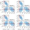 |
Fig. 1. Constraints on sound horizon rd, Hubble constant H0 and Ωk from late-time observations including BAO (BOSS), type Ia supernovae (Pantheon), gravitational lensing (H0LiCOW) and cosmic distance ladder calibrated with Cepheids (SH0ES). The panels show results for three cosmology-independent models listed in Table 1 and a ΛCDM cosmological model. The red lines indicate the best fit values obtained from Planck for a flat ΛCDM cosmological model. The contours indicate 1-, 2- and 5σ confidence regions of the posterior probability (the latter obtained by Gaussian extrapolation). All panels demonstrate a 5σ tension between rd and H0 measured from the CMB and the late-time observations. |
Posterior mean and standard deviation for the sound horizon rd, H0rd and q0 inferred from late-time observations including H0LiCOW lensing observations, Pantheon SN sample, and BAO measurements (BOSS).
In Table 4, some other combinations of data sets are explored. This includes a calibration of lenses + CCHP instead of SH0ES, inclusion of several volume-averaged and Ly-α BAO and the addition of high redshift quasars as secondary standard candles. Considering all results based on the main data sets (H0LiCOW, SN, BAO/BOSS) with the cosmic distance ladder (SH0ES or CCHP), we find rd = (137 ± 3stat. ± 2syst.) Mpc, where the systematic error accounts for differences between SH0ES and CCHP distance calibration. In addition, we ran an inference free of any SN data, thus only using lensed quasars and BAO measurements from BOSS, DV and Ly-α with a flat ΛCDM model6 This results in the following values for the cosmological parameters: rd = 138.6 ± 3.8 Mpc, H0rd = 10166 ± 142 km s−1, Ωm = 0.29 ± 0.02.
4.1. Early-time extensions
A possible solution for the tension is an extension to the early Universe physics, such as an additional component of relativistic species. Planck 2018 chains with free Neff (based on full temperature and polarisation data) were used to investigate this scenario. In Fig. 2, Planck + free Neff is compared to results from model 3 using SN + BAO with only the H0LiCOW lenses as calibrator (upper panel) and using a combination of H0LiCOW lenses and either SH0ES or CCHP as calibrators (lower panel). A higher value of Neff is shown to move the Planck value to a lower rd and a higher H0, therefore alleviating the tension to some extent. In this case, the combined analysis of Planck and low-redshift data yields Neff = 3.24 ± 0.16. This effect is only convincing when the late-time measurements are calibrated with H0LiCOW and CCHP, since the alternative Cepheid calibration is still in tension with the Planck +Neff extension (see Table 3).
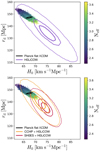 |
Fig. 2. Comparison between sound horizon rd and Hubble constant H0 measured from Planck observations of the CMB (assuming a flat ΛCDM) and late-time observations (using flat model 3) obtained by calibrating SN and BAO measurements with three different absolute distance calibrations from: gravitational lensing (H0LiCOW), the cosmic distance ladder with Cepheids (SH0ES) or the TRGB (CCHP). For the late-time data, the contours show 1-, 2- and 5σ confidence regions of the posterior probability (the latter obtained by Gaussian extrapolation). The Planck constraints (1- and 2σ confidence regions) are obtained for the standard effective number of neutrinos (black solid line) and a model with a free effective number of neutrinos (black dashed lines, colour points). |
4.2. Tension between the CMB and late-time observations
Figure 3 demonstrates the potential of the selected extensions of the standard ΛCDM model outlined in Sect. 3.2 to resolve the tension between rd and H0 measured from the CMB and late-time observations. The shaded grey contours show constraints from late-time observations using model 3 with Ωk = 0. Thanks to a polynomial parametrisation, these measurements are marginalised over a wide class of the expansion history and in this sense they are independent of cosmological model. We show results for distance calibrations based on the H0LiCOW lenses combined with SH0ES or CCHP. The contours in colour show constraints from Planck for the flat ΛCDM model (black contours) and its four extensions.
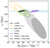 |
Fig. 3. Effects of four different extensions of the flat ΛCDM model on the sound horizon and the Hubble constant measured from the Planck data. The models considered here are ΛCDM + free Neff, early dark energy, wCDM, and PEDE. The CMB-based constraints are compared to the measurements from late-time observations (SN + BAO + H0LiCOW + SH0ES/CCHP) shown with the grey shaded contours. The late-time measurements are obtained with model 3 (see Table 1) and show the 2σ credibility regions. |
As clearly seen from Fig. 3, none of the ΛCDM extensions manage to convincingly unify the Planck measurements with the late-time ones if the SH0ES calibration is used to anchor the distance ladder. In particular, late-time extensions involving different generalisations of the cosmological constant can increase the H0 value inferred from the CMB, but they leave rd unchanged. Although early-time extensions can potentially match both H0 and rd from low-redshift probes and the CMB, that this may happen by expanding the posterior probability contours rather than shifting the best fit values (see also Bernal et al. 2016; Karwal & Kamionkowski 2016), as demonstrated in Fig. 3. In this respect, both early dark energy models and extensions with extra relativistic species are quite similar. The apparent difference between their probability contours reflect differences in the priors. While a free effective number of relativistic species can either decrease or increase the sound horizon, early dark energy (with positive energy density) can only increase the energy budget, and thus decrease the sound horizon.
Figure 4 summarises the tension in the H0 − rd plane between late-time measurements and Planck with different extensions of ΛCDM. To ensure a fair comparison, the same ΛCDM extensions are used in the late-time and CMB-based inference. Therefore, the Planck PEDE-CDM results have been compared to late-time results obtained with PEDE-CDM, and the Planck wCDM results to late-time results using wCDM. For the early-time extensions, this is not of great importance, since their effects do not influence the low-redshift measurements.
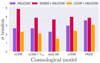 |
Fig. 4. Tension between sound horizon and Hubble constant measured from late-time observations and CMB for the following cosmological models: ΛCDM, ΛCDM + Neff, early DE, wCDM, PEDE-CDM (flatness assumed in all cases). Late-time observations include BAO, type Ia supernovae, and three different absolute distance calibrations from gravitational lensing (H0LiCOW), the cosmic distance ladder with Cepheids (SH0ES) or the TRGB (CCHP). |
By adopting different models of polynomial parametrisations (models 1, 2, and 3), we minimised the dependence on a cosmological model. Although our inference with these models does not depend on ΛCDM, it does have a weak dependency on general relativity (GR). The lensed quasars that are used to calibrate the distance ladder need GR in order to calculate the angular diameter distance, through the Ansatz that the lensing potential (used in the time-delay inference) is exactly twice the gravitational potential (used to obtain DA ∝ c3 Δt/σ2 from stellar kinematics). However, the role of this GR dependence is subdominant with current DA uncertainties (10%−20%). On the other hand, GR also enters the early-Universe expansion through the “abundances” of different components (ΩmΩde, Neff).
4.3. One lens at a time
Since H0 and rd are constants, they must be independent of the chosen indicators. If they are inferred from each indicator separately, any trend will signal residual systematics, either in the indicators themselves or in the parametrisation that is chosen to extrapolate H(z) down to H0.
The H0LiCOW collaboration has shown that if H0 is obtained from lenses in a flat-ΛCDM model, there is a weak trend in its inferred value versus redshift. Lenses of lower (higher) redshift differ more (less) from the Planck measurements (Wong et al. 2020). Even though this trend is currently not significant (given current uncertainties), it may be indicative of intrinsic systematics in the lensing inference, or in the way that time-delay distances are converted into H0 values through a flat-ΛCDM parametrisation.
Here, we repeat this test using more general models of the expansion history, specifically flat model 3 and flat PEDE-CDM model. Figure 5 shows the sound horizon rd measured from combining BAO and SNe data with lensing constraints from each lens separately. The results demonstrate that the distance calibration from H0LiCOW lenses shows a similar trend with lens redshift as the one shown by Wong et al. (2020) for a flat ΛCDM cosmology. Based on the sample-wide analysis by Millon et al. (2020), this weak trend cannot be explained simply on the basis of known systematics in the lens models or kinematics of each lens. We should emphasise, however, that this trend is not statistically significant (1.6σ) yet.
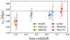 |
Fig. 5. Sound horizon rd measured from combining BAO and SNe data with H0LiCOW lensing observations of each lens separately. Here, the distance calibration is set solely by the lensing observations of each individual lens. The measured sound horizon is shown as a function of lens redshift for fits with a flat model 3 (solid error bars) and a flat PEDE-CDM model (dashed error bars). For both models, the measurements show a slight trend of rd increasing with lens redshift. The inference from models 1 and 2 is fully consistent with the model 3 results. The grey dashed line with shaded region shows Planck’s value of rd and its (sub-percent) uncertainty obtained for the standard flat ΛCDM model. |
Although the current weak trend of rd with redshift of gravitatonal lens is consistent with being a statistical fluke, it is instructive to investigate if there any expansion models that can re-absorb this (weak) trend. For example, a recent (z ≈ 0.4) change in dark energy may produce this behaviour, if the data are interpreted with expansion histories that are “too” smooth. For this reason, we examined the same lens-by-lens determination within the PEDE model family. The results are shown as dotted error-bars in Fig. 5. Even the PEDE model with accelerated late-time expansion cannot eliminate the (weak) trend in rd. The constraints set by the relative distance moduli of SN enforce PEDE to closely resemble the ΛCDM case, but with a higher matter content (Ωm ≈ 0.345) and smaller sound horizon (rd ≈ 138 Mpc). Therefore, PEDE does not resolve the current tension.
5. Conclusions and outlook
We combined the newest available low-redshift probes to obtain an estimate of the sound horizon at the drag epoch, rd. In order to minimise the dependence on a cosmological model, we used a set of polynomial parametrisations that are almost entirely independent of the underlying cosmology, as well as the standard ΛCDM model. In the H0 − rd plane, we found a tension of 5σ between Planck results using flat ΛCDM and late-time observations calibrated with H0LiCOW lenses and SH0ES. This tension is reduced to 2.4σ if CCHP results are used as a distance-ladder anchor instead of SH0ES. We investigated whether early- or late-time extensions to the standard ΛCDM model can resolve the tension, and we examined models with free Neff, early dark energy, wCDM, and PEDE-CDM. None of these model extensions provide a satisfying solution to the Hubble tension problem (see also Aylor et al. 2019; Knox & Millea 2020), except for free Neff or early dark energy in combination with low redshift data calibrated by CCHP + H0LiCOW.
These findings may indicate that: (1) extensions of early-time physics are necessary; and/or (2) that systematics from different late-time probes are becoming comparable to the statistical uncertainties. Arguments based on local under-densities or peculiar velocities cannot resolve the tension: the ≈3σ tension persists if the inverse-distance ladder is restricted to z ≥ 0.03, where the role of peculiar velocities is ≲0.1% (see also Wojtak & Agnello 2019). Multiple secondary sources of errors in redshift measurements were studied by Davis et al. (2019), but none of them seem to have any noticeable effect. Another explanation may be that the standardisation of SNe Ia is not properly understood yet (as a caveat, see Rigault et al. 2015, for example, or Khetan et al. 2020), or that there is some (hitherto undiscovered) source of systematics in one of the other used data sets. If all astrophysical systematics are exhausted, one can also consider proposals involving non-standard physics in the local Universe such as screened fifth forces, which may bias H0 measurements high via modulation of gravity-dependent pulsation periods of Cepheids (for more details see Desmond et al. 2019). For these reasons, we also provide a measurement that relies only on lenses and BAO, without any additional constraint from SNe, in Sect. 4.
The weak trend in Fig. 5 may indicate residual systematics in the lens models, or the need for different low-z expansion models, or it may vanish entirely with larger lens samples. In order to check the robustness of the trend, cosmography-grade models of more lenses are needed, over the whole 0.3 ≲ z ≲ 0.7 current redshift interval and beyond. Finally, the role of systematics in the lens-mass models can be assessed once high-S/N spatially resolved kinematics are available (Shajib et al. 2018; Yıldırım et al. 2020), which would enable more flexible dynamical models than the ones used so far on aperture-averaged velocity dispersions.
As a final remark, we emphasise that resolving the H0 tension alone is not sufficient, since different models that can shift this value are still at tension with the inferred rd from BAO and low-redshift indicators. Also, a direct combination of the inference from late-time and CMB-based measurements that may be at > 3σ tension, hence hardly compatible with one another, should be justified. Therefore, any new proposal to resolve the discrepancy between CMB-based and late-time measurements should consider both H0 and rd, and examine the separate inference upon late-time and CMB-based data.
Where the distance measures are related to each other according to DL = (1 + z)DM = (1 + z)2DA.
Full names and coordinates of each lens are given in the H0LiCOW XIII paper (Wong et al. 2020).
DΔt = (1 + zl)DA, lDA, s/DA, ls, where DA, l, DA, s and DA, ls are the angular distance to the lens galaxy, lensed quasar, and between the lens and the quasar; zl is redshift of the lens galaxy.
For the flat ΛCDM model, we adopted a prior of ΩM = 𝒰[0.05, 0.5].
Here, log(1 + z) refers to the log base 10, and not to the natural logarithm.
Acknowledgments
We thank Chiara Spiniello for useful comments on an earlier version of this manuscript, and Inh Jee and Eiichiro Komatsu for discussions on the lensing distance likelihoods. These time delay cosmography observations are associated with programs HST-GO-9375, HST-GO-9744, HST-GO-10158, HST-GO-12889, and HST-14254. Support for programs HST-GO-10158 HST-GO-12889 HST-14254 was provided to members of our team by NASA through grants from the Space Telescope Science Institute, which is operated by the Association of Universities for Research in Astronomy, Inc., under NASA contract NAS 5-26555. AA and RJW were supported by a grant from VILLUM FONDEN (project number 16599). This project is partially funded by the Danish council for independent research under the project “Fundamentals of Dark Matter Structures”, DFF–6108-00470. This project has received funding from the European Research Council (ERC) under the EU’s Horizon 2020 research and innovation programme (COSMICLENS; grant agreement No. 787886) and from the Swiss National Science Foundation (SNSF). This work was supported by World Premier International Research Center Initiative (WPI Initiative), MEXT, Japan. SH acknowledges support by the DFG cluster of excellence “Origin and Structure of the Universe” (www.universe-cluster.de). CDF acknowledges support for this work from the National Science Foundation under Grant No. AST-1715611. SHS thanks the Max Planck Society for support through the Max Planck Research Group. TT acknowledges support by the Packard Foundation through a Packard Research fellowship and by the National Science Foundation through NSF grants AST-1714953 and AST-1906976. LVEK is partly supported through an NWO-VICI grant (project number 639.043.308).
References
- Addison, G. E., Watts, D. J., Bennett, C. L., et al. 2018, ApJ, 853, 119 [Google Scholar]
- Alam, S., Ata, M., Bailey, S., et al. 2017, MNRAS, 470, 2617 [NASA ADS] [CrossRef] [Google Scholar]
- Arendse, N., Agnello, A., & Wojtak, R. J. 2019, A&A, 632, A91 [CrossRef] [EDP Sciences] [Google Scholar]
- Ata, M., Baumgarten, F., Bautista, J., et al. 2018, MNRAS, 473, 4773 [NASA ADS] [CrossRef] [Google Scholar]
- Aylor, K., Joy, M., Knox, L., et al. 2019, ApJ, 874, 4 [NASA ADS] [CrossRef] [Google Scholar]
- Bautista, J. E., Vargas-Magaña, M., Dawson, K. S., et al. 2018, ApJ, 863, 110 [NASA ADS] [CrossRef] [Google Scholar]
- Bernal, J. L., Verde, L., & Riess, A. G. 2016, J. Cosmology Astropart. Phys, 10, 019 [Google Scholar]
- Blomqvist, M., du Mas des Bourboux, H., & Busca, N. G. 2019, A&A, 629, A86 [NASA ADS] [CrossRef] [EDP Sciences] [Google Scholar]
- Bonvin, V., Millon, M., Chan, J. H. H., et al. 2019, A&A, 629, A97 [NASA ADS] [CrossRef] [EDP Sciences] [Google Scholar]
- Carneiro, S., de Holanda, P. C., Pigozzo, C., & Sobreira, F. 2019, Phys. Rev. D, 100, 023505 [CrossRef] [Google Scholar]
- Carter, P., Beutler, F., Percival, W. J., et al. 2018, MNRAS, 481, 2371 [CrossRef] [Google Scholar]
- Cattoën, C., & Visser, M. 2007, CQG, 24, 5985 [Google Scholar]
- Chen, G. C. F., Fassnacht, C. D., Suyu, S. H., et al. 2019, MNRAS, 490, 1743 [Google Scholar]
- Cuceu, A., Farr, J., Lemos, P., & Font-Ribera, A. 2019, J. Cosmology Astropart. Phys., 2019, 044 [CrossRef] [Google Scholar]
- Davis, T. M., Hinton, S. R., Howlett, C., & Calcino, J. 2019, MNRAS, 490, 2948 [NASA ADS] [CrossRef] [Google Scholar]
- de Sainte Agathe, V., Balland, C., & du Mas des Bourboux, H. 2019, A&A, 629, A85 [NASA ADS] [CrossRef] [EDP Sciences] [Google Scholar]
- Desmond, H., Jain, B., & Sakstein, J. 2019, Phys. Rev. D, 100, 043537 [NASA ADS] [CrossRef] [Google Scholar]
- Doran, M., Stern, S., & Thommes, E. 2007, J. Cosmology Astropart. Phys., 2007, 015 [Google Scholar]
- Eisenstein, D., & White, M. 2004, Phys. Rev. D, 70, 103523 [NASA ADS] [CrossRef] [Google Scholar]
- Foreman-Mackey, D., Hogg, D. W., Lang, D., & Goodman, J. 2013, PASP, 125, 306 [CrossRef] [Google Scholar]
- Freedman, W. L., Madore, B. F., Hatt, D., et al. 2019, ApJ, 882, 34 [NASA ADS] [CrossRef] [Google Scholar]
- Freedman, W. L., Madore, B. F., Hoyt, T., et al. 2020, ApJ, 891, 57 [Google Scholar]
- Gelmini, G. B., Kusenko, A., & Takhistov, V. 2019, ArXiv e-prints [arXiv:1906.10136] [Google Scholar]
- Goodman, J., & Weare, J. 2010, Commun. Appl. Math. Comput. Sci., 5, 65 [Google Scholar]
- Hannestad, S. 2003, J. Cosmology Astropart. Phys., 2003, 004 [NASA ADS] [CrossRef] [Google Scholar]
- Heavens, A., Jimenez, R., & Verde, L. 2014, Phys. Rev. Lett., 113, 241302 [NASA ADS] [CrossRef] [Google Scholar]
- Hu, W., & Sugiyama, N. 1996, ApJ, 471, 542 [NASA ADS] [CrossRef] [Google Scholar]
- Jee, I., Suyu, S. H., Komatsu, E., et al. 2019, Science, 365, 1134 [CrossRef] [Google Scholar]
- Karwal, T., & Kamionkowski, M. 2016, Phys. Rev. D, 94, 103523 [CrossRef] [Google Scholar]
- Kazin, E. A., Koda, J., Blake, C., et al. 2014, MNRAS, 441, 3524 [NASA ADS] [CrossRef] [Google Scholar]
- Knox, L., & Millea, M. 2020, Phys. Rev. D, 101, 043533 [CrossRef] [Google Scholar]
- Li, E.-K., Du, M., & Xu, L. 2020, MNRAS, 491, 4960 [Google Scholar]
- Li, X., & Shafieloo, A. 2019, ApJ, 883, L3 [CrossRef] [Google Scholar]
- Linder, E. V., & Robbers, G. 2008, J. Cosmology Astropart. Phys., 2008, 004 [CrossRef] [Google Scholar]
- Millon, M., Galan, A., Courbin, F., et al. 2020, A&A, in press, https://doi.org/10.1051/0004-6361/201937351 [Google Scholar]
- Mörtsell, E., & Dhawan, S. 2018, J. Cosmology Astropart. Phys., 2018, 025 [NASA ADS] [CrossRef] [Google Scholar]
- Planck Collaboration VI. 2020, A&A, in press https://doi.org/10.1051/0004-6361/201833910 [Google Scholar]
- Poulin, V., Smith, T. L., Grin, D., Karwal, T., & Kamionkowski, M. 2018, Phys. Rev. D, 98, 083525 [CrossRef] [Google Scholar]
- Poulin, V., Smith, T. L., Karwal, T., & Kamionkowski, M. 2019, Phys. Rev. Lett., 122, 221301 [NASA ADS] [CrossRef] [Google Scholar]
- Riess, A. G., Casertano, S., Yuan, W., Macri, L. M., & Scolnic, D. 2019, ApJ, 876, 85 [NASA ADS] [CrossRef] [Google Scholar]
- Rigault, M., Aldering, G., Kowalski, M., et al. 2015, ApJ, 802, 20 [NASA ADS] [CrossRef] [Google Scholar]
- Risaliti, G., & Lusso, E. 2019, Nat. Astron., 3, 272 [NASA ADS] [CrossRef] [Google Scholar]
- Rusu, C. E., Wong, K. C., & Bonvin, A. 2019, MNRAS, stz3451 [Google Scholar]
- Scolnic, D. M., Jones, D. O., Rest, A., et al. 2018, ApJ, 859, 101 [NASA ADS] [CrossRef] [Google Scholar]
- Shajib, A. J., Treu, T., & Agnello, A. 2018, MNRAS, 473, 210 [NASA ADS] [CrossRef] [Google Scholar]
- Sluse, D., Rusu, C. E., Fassnacht, C. D., et al. 2019, MNRAS, 490, 613 [Google Scholar]
- Suyu, S. H., Bonvin, V., Courbin, F., et al. 2017, MNRAS, 468, 2590 [Google Scholar]
- Taubenberger, S., Suyu, S. H., Komatsu, E., et al. 2019, A&A, 628, L7 [NASA ADS] [CrossRef] [EDP Sciences] [Google Scholar]
- Verde, L., Protopapas, P., & Jimenez, R. 2013, Phys. Dark Univ., 2, 166 [Google Scholar]
- Verde, L., Bernal, J. L., Heavens, A. F., & Jimenez, R. 2017, MNRAS, 467, 731 [NASA ADS] [Google Scholar]
- Visser, M. 2004, CQG, 21, 2603 [NASA ADS] [CrossRef] [MathSciNet] [Google Scholar]
- Weinberg, S. 1972, Gravitation and Cosmology: Principles and Applications of the General Theory of Relativity (Wiley-VCH) [Google Scholar]
- Wojtak, R., & Agnello, A. 2019, MNRAS, 486, 5046 [NASA ADS] [CrossRef] [Google Scholar]
- Wong, K. C., Suyu, S. H., Chen, G. C. F., et al. 2020, MNRAS, in press [arXiv:1907.04869] [Google Scholar]
- Yang, T., Banerjee, A., & Colgáin, E. 2019, ArXiv e-prints [arXiv:1911.01681] [Google Scholar]
- Yıldırım, A., Suyu, S. H., & Halkola, A. 2020, MNRAS, 493, 4783 [CrossRef] [Google Scholar]
- Yuan, W., Riess, A. G., Macri, L. M., Casertano, S., & Scolnic, D. M. 2019, ApJ, 886, 61 [CrossRef] [Google Scholar]
Appendix A: Planck compressed likelihood
Much of the constraining power of the CMB power spectrum can be compressed in three parameters: the physical density of baryons Ωbh2, which determines relative heights of the peaks in the power spectrum, and two so-called shift parameters that describe two fundamental and directly measured angular scales related to the sound horizon and the Hubble horizon at the time of decoupling. The shift parameters are defined by the following equations:
 (A.1)
(A.1)
 (A.2)
(A.2)
where z* is redshift of decoupling and DA is the comoving angular diameter distance, which for flat models considered in this work is given by
 (A.3)
(A.3)
![Mathematical equation: $$ \begin{aligned}&H^{2}(z) = H_{0}^{2}[\Omega _{\rm m}(1+z)^{3}+\Omega _{\rm DE}(z)+\Omega _{\gamma }(1+z)^{4}], \end{aligned} $$](/articles/aa/full_html/2020/07/aa36720-19/aa36720-19-eq19.gif) (A.4)
(A.4)
where Ωγ denotes the density parameter of radiation, meaning Ωγ = 2.47 × 10⁻⁵h−2.
The comoving sound horizon is given by
 (A.5)
(A.5)
Here, an additional contribution to the energy density driving the expansion comes from relativistic neutrinos. The density parameter of relativistic neutrinos Ωn is given by
 (A.6)
(A.6)
where Neff is the effective number of neutrinos, with Neff = 3.046 for the baseline model.
We computed redshift z* of decoupling employing the following fitting formula (Hu & Sugiyama 1996):
![Mathematical equation: $$ \begin{aligned} z_{*}&= 1047[1+0.00124(\Omega _{\rm b}h^{2})^{-0.738}][1+g_{1}(\Omega _{\rm m}h^{2})^{g_{2}}] \end{aligned} $$](/articles/aa/full_html/2020/07/aa36720-19/aa36720-19-eq22.gif) (A.7)
(A.7)
![Mathematical equation: $$ \begin{aligned} g_{1}&= 0.0783(\Omega _{\rm b}h^{2})^{-0.238}[1+39.5(\Omega _{\rm b}h^{2})^{0.763}]^{-1}\end{aligned} $$](/articles/aa/full_html/2020/07/aa36720-19/aa36720-19-eq23.gif) (A.8)
(A.8)
![Mathematical equation: $$ \begin{aligned} g_{2}&= 0.56[1+21.1(\Omega _{\rm b}h^{2})^{1.81}] . \end{aligned} $$](/articles/aa/full_html/2020/07/aa36720-19/aa36720-19-eq24.gif) (A.9)
(A.9)
The sound horizon imprinted in galaxy clustering and measured from BAO observations is fixed at the drag epoch, when the baryons are released from the Compton drag of the photons. The corresponding drag redshift zd can be calculated using the following fitting function (Hu & Sugiyama 1996):
![Mathematical equation: $$ \begin{aligned} z_{\rm d}&= 1345\frac{(\Omega _{\rm m}h^{2})^{0.251}[1+b_{1}(\Omega _{\rm b}h^{2})^{b_{2}})]}{ 1+0.659(\Omega _{\rm m}h^{2})^{0.828}} \end{aligned} $$](/articles/aa/full_html/2020/07/aa36720-19/aa36720-19-eq25.gif) (A.10)
(A.10)
![Mathematical equation: $$ \begin{aligned} b_{1}&= 0.313(\Omega _{\rm m}h^{2})^{-0.419}[1+0.607(\Omega _{\rm m}h^{2})^{0.674}]\end{aligned} $$](/articles/aa/full_html/2020/07/aa36720-19/aa36720-19-eq26.gif) (A.11)
(A.11)
 (A.12)
The compressed CMB likelihood is given by a three-dimensional Gaussian distribution in the three parameters mentioned above, meaning Ωnh2, ℛ, and θ*. We employed the mean values and the covariance matrix determined from publicly available MCMC models obtained for a flat ΛCDM model fitted to the Planck observations, including the temperature, polarisation, and lensing data (Planck Collaboration VI 2020): (100Ωbh2, 100θ*, ℛ) = (2.237 ± 0.015, 1.0411 ± 0.00031, 1.74998 ± 0.004) with the following correlation matrix:
 (A.13)
The compressed likelihood accurately recovers the actual constraints obtained from the complete likelihood for a flat ΛCDM model (see Fig. A.1). Only a fine adjustment of the redshift scales in both fitting formulae (δz/z ∼ 10−3, smaller relative to the values adopted in Hu & Sugiyama 1996) was applied in order to correct for a sub-percent bias in the mean values of relevant parameters. In general, both approximations used to compute z* and zdrag are accurate to within 1 per cent in a wide range of the matter and baryon density parameters (Hu & Sugiyama 1996).
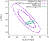 |
Fig. A.1. Comparison between constraints on rd and H0 from the full Planck likelihood (dashed lines) and the compressed likelihood (for post-recombination modifications of ΛCDM) or the extended compressed likelihood (for pre-recombination modifications of ΛCDM) used in this study (solid lines). The robustness test comprises two cases: the standard flat ΛCDM model and its extension with a free number of neutrinos. |
For early-time extensions of the standard ΛCDM cosmology (such as a model with free Neff), the compressed likelihood turns out to be insufficient, leading to a family of models with a wide range of amplitudes of the first peak in the power spectrum. In order to circumvent this problem, we extended the compressed likelihood described above by accounting for the height of the first peak in the power spectrum as an additional constraint. Bearing in mind that the amplitude scales with Ωdmh2, meaning the physical density of dark matter, a simple extension relies on adding Ωdmh2 as the fourth variable in the compressed likelihood function. Using Planck results for a ΛCDM model with a free effective number of neutrinos as a base early-time extension (inferred from the full temperature and polarisation data), we determined the mean values and the covariance matrix of the new four-parameter compressed likelihood, obtaining (100Ωbh2, 100θ*, ℛ, Ωdmh2) = (2.225 ± 0.0223, 1.0414 ± 0.00054, 1.7529 ± 0.0056, 0.1184 ± 0.0029) and the following correlation matrix:
 (A.14)
Figure A.1 demonstrates that the extended compressed likelihood accurately recovers the actual constraints on rd and H0 from Planck for a model with a free effective number of neutrinos.
Appendix B: Polynomial parametrisations
This section gives more detailed information about the polynomial parametrisations used throughout this work.
B.1. Expansion formulae
Our first model is the simplest one and adopts a polynomial expansion of H(z) in z;
![Mathematical equation: $$ \begin{aligned} {{H(z) = H_0 \left[ 1 + b_1 \, z + b_2 \, z^2 + \mathcal{O} (z^3)\right],}} \end{aligned} $$](/articles/aa/full_html/2020/07/aa36720-19/aa36720-19-eq30.gif) (B.1)
(B.1)
where H0 is the Hubble constant, and the coefficient b1 is related to the deceleration parameter q0 through
 (B.2)
(B.2)
In our second model, the luminosity distance DL is expanded as a polynomial in log(1 + z)7;
![Mathematical equation: $$ \begin{aligned}&{x = \log (1+z),} \nonumber \\&{D_L (z) = \frac{c \, \ln (10)}{H_0} \left[ x + c_2 x^2 + c_3 x^3 + c_4 x^4 + \mathcal{O} (x^5) \right],} \end{aligned} $$](/articles/aa/full_html/2020/07/aa36720-19/aa36720-19-eq32.gif) (B.3)
(B.3)
where the coefficient c2 is related to the deceleration parameter through the following relation:
 (B.4)
(B.4)
This different parametrisation was chosen in order to avoid convergence problems with the Taylor expansion around zero, when employing data with redshifts z > 1. By introducing a new variable x that satisfies x = 0 when z = 0, and x < 1 when z → 2 (where the upper limit of 2 is based on the highest lensed quasar redshift), the parametrisation is kept within the convergence radius of the Taylor expansion.
Our third model describes transverse comoving distances DM by polynomials in z/(1 + z);
![Mathematical equation: $$ \begin{aligned}&{y = \frac{z}{1+z},} \nonumber \\&{D_M (z) = \frac{c}{H_0} \left[ { y} + d_2 { y}^2 + d_3 { y}^3 + d_4 { y}^4 + \mathcal{O} ({ y}^5) \right],} \end{aligned} $$](/articles/aa/full_html/2020/07/aa36720-19/aa36720-19-eq34.gif) (B.5)
(B.5)
where the coefficient d2 is related to the deceleration parameter through
 (B.6)
(B.6)
This parametrisation was, similarly to the one in model 2, chosen to overcome convergence problems.
B.2. Truncation of the polynomials
An important thing to consider is at which order the Taylor expansions should be truncated. Higher orders of expansions can give better approximations to the shape of the data, but also introduce more free parameters and therefore larger uncertainties. In order to determine the truncation of the polynomials as given in Eqs. (B.1), (B.3), and (B.5), we performed a convergence test to check that the models can accurately recover expansion history of a fiducial flat ΛCDM cosmological model in a redshift range of observational data used in our study, for instance, z < 1.8. The test relies on comparing distances from models 1–3 to the actual distances in the fiducial model. Free parameters of the models were determined by matching coefficients of Taylor expanded Hubble parameter in models 1–3 and the fiducial model. The latter yields well-known kinematical coefficients (Weinberg 1972; Visser 2004):
 (B.7)
(B.7)
Since the errors that we obtain by combining calibrations of H0LiCOW and SH0ES are around 2% (see Table 3), we required our models to be within a 2% accuracy of ΛCDM distances in this test. The results can be seen in Fig. B.1 for Ωm = 0.3, where the shaded region corresponds to this imposed limit. It is sufficient to employ three free parameters (corresponding to a second-order polynomial) for model 1 and four free parameters (corresponding to a fourth-order polynomial) for models 2 and 3 to satisfy the convergence condition. Since a further increase of the number of free parameters is disfavoured by the BIC obtained in fits with the actual late-time observations, these polynomial truncations were adopted in our study (see Table 1). The BIC score is calculated as
 (B.8)
(B.8)
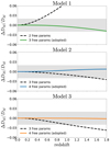 |
Fig. B.1. Relative differences between distances in a fiducial flat ΛCDM model and distances derived from models 1-3 with free parameters matched to the kinematical coefficients of the fiducial model, ΔDM/DM = (DM, expansion − DM, ΛCDM)/DM, ΛCDM. The solid lines show the results satisfying the convergence criterion, which sets the truncation of polynomials used in the adopted models in this study. |
where N is the number of data points and k is the number of all free parameters in the cosmological fits.
B.3. Test with mock distance-modulus data
As a final test for our polynomial parametrisation models, we investigated if any biases were introduced when we fitted models 1-3 to flat ΛCDM data. We transformed the Pantheon SN data set to a mock data set by replacing their binned distance modulus entries with the fiducial flat ΛCDM values (adopting H0 = 74 km s−1 Mpc−1 and Ωm = 0.3) at the same redshifts. For the errors associated with the distance moduli we keep the original Pantheon ones. By construction, best fit ΛCDM parameters are equal to their fiducial values, whereas relative shifts in best fit parameters obtained for non-ΛCDM models measure the corresponding biases. This test is similar to the one performed by Yang et al. (2019), in which they found that our model 2 introduces an artificial bias. However, their mock data set is based on Pantheon data as well as high-redshift quasar and GRB data (with zmax = 6.7), while in our work we only used sources below z = 1.8. Figure B.2 shows the best fit values for the coefficients bi, ci, and di of models 1-3, obtained with MCMC, and their true values in a flat ΛCDM cosmology. As can be seen, they are in complete agreement with each other. In fact, the relative difference in H0 between the fiducial value and those of models 1-3 is 0.03%, 0.02%, and 0.02%, respectively. This bias is about a hundred times smaller than the current precision achieved by SH0ES and H0LiCOW data (which is around 2%). The bias in q0 is larger: 2.0%, 1.2%, and 1.3% for models 1-3, but still negligible compared to our obtained errors in q0 (which are 10% at best).
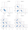 |
Fig. B.2. Best-fit values of flat ΛCDM and polynomial parametrisation models 1-3 to mock data. The mock data is generated by replacing the Pantheon distance modulus points by their fiducial flat ΛCDM values. The red lines indicate the canonical ΛCDM values of Ωm, H0 and the expansion coefficients bi, ci, and di. |
This test demonstrates that if the underlying cosmology is flat ΛCDM, then our models will not introduce any significant biases in the Pantheon redshift range. The convergence test in the previous section also guarantees this. The bias that Yang et al. (2019) found in their model was a consequence of it not passing the convergence test over the complete redshift range of z = 0 − 7.
We repeated the test for the PEDE model and for a wCDM cosmology with w = −1.2. In both cases, we assumed Ωm = 0.3. We found only a sub-percent bias in the best fit H0 and a few-percent bias in q0, where the actual values are given by;
 (B.9)
(B.9)
All Tables
Three polynomial parametrisations (models 1, 2, and 3) adopted in this study to place cosmology-independent constraints on rd and H0.
Posterior mean and standard deviation for the sound horizon rd, H0rd and q0 inferred from late-time observations including H0LiCOW lensing observations, Pantheon SN sample, and BAO measurements (BOSS).
All Figures
|
Fig. 1. Constraints on sound horizon rd, Hubble constant H0 and Ωk from late-time observations including BAO (BOSS), type Ia supernovae (Pantheon), gravitational lensing (H0LiCOW) and cosmic distance ladder calibrated with Cepheids (SH0ES). The panels show results for three cosmology-independent models listed in Table 1 and a ΛCDM cosmological model. The red lines indicate the best fit values obtained from Planck for a flat ΛCDM cosmological model. The contours indicate 1-, 2- and 5σ confidence regions of the posterior probability (the latter obtained by Gaussian extrapolation). All panels demonstrate a 5σ tension between rd and H0 measured from the CMB and the late-time observations. |
| In the text | |
|
Fig. 2. Comparison between sound horizon rd and Hubble constant H0 measured from Planck observations of the CMB (assuming a flat ΛCDM) and late-time observations (using flat model 3) obtained by calibrating SN and BAO measurements with three different absolute distance calibrations from: gravitational lensing (H0LiCOW), the cosmic distance ladder with Cepheids (SH0ES) or the TRGB (CCHP). For the late-time data, the contours show 1-, 2- and 5σ confidence regions of the posterior probability (the latter obtained by Gaussian extrapolation). The Planck constraints (1- and 2σ confidence regions) are obtained for the standard effective number of neutrinos (black solid line) and a model with a free effective number of neutrinos (black dashed lines, colour points). |
| In the text | |
|
Fig. 3. Effects of four different extensions of the flat ΛCDM model on the sound horizon and the Hubble constant measured from the Planck data. The models considered here are ΛCDM + free Neff, early dark energy, wCDM, and PEDE. The CMB-based constraints are compared to the measurements from late-time observations (SN + BAO + H0LiCOW + SH0ES/CCHP) shown with the grey shaded contours. The late-time measurements are obtained with model 3 (see Table 1) and show the 2σ credibility regions. |
| In the text | |
|
Fig. 4. Tension between sound horizon and Hubble constant measured from late-time observations and CMB for the following cosmological models: ΛCDM, ΛCDM + Neff, early DE, wCDM, PEDE-CDM (flatness assumed in all cases). Late-time observations include BAO, type Ia supernovae, and three different absolute distance calibrations from gravitational lensing (H0LiCOW), the cosmic distance ladder with Cepheids (SH0ES) or the TRGB (CCHP). |
| In the text | |
|
Fig. 5. Sound horizon rd measured from combining BAO and SNe data with H0LiCOW lensing observations of each lens separately. Here, the distance calibration is set solely by the lensing observations of each individual lens. The measured sound horizon is shown as a function of lens redshift for fits with a flat model 3 (solid error bars) and a flat PEDE-CDM model (dashed error bars). For both models, the measurements show a slight trend of rd increasing with lens redshift. The inference from models 1 and 2 is fully consistent with the model 3 results. The grey dashed line with shaded region shows Planck’s value of rd and its (sub-percent) uncertainty obtained for the standard flat ΛCDM model. |
| In the text | |
|
Fig. A.1. Comparison between constraints on rd and H0 from the full Planck likelihood (dashed lines) and the compressed likelihood (for post-recombination modifications of ΛCDM) or the extended compressed likelihood (for pre-recombination modifications of ΛCDM) used in this study (solid lines). The robustness test comprises two cases: the standard flat ΛCDM model and its extension with a free number of neutrinos. |
| In the text | |
|
Fig. B.1. Relative differences between distances in a fiducial flat ΛCDM model and distances derived from models 1-3 with free parameters matched to the kinematical coefficients of the fiducial model, ΔDM/DM = (DM, expansion − DM, ΛCDM)/DM, ΛCDM. The solid lines show the results satisfying the convergence criterion, which sets the truncation of polynomials used in the adopted models in this study. |
| In the text | |
|
Fig. B.2. Best-fit values of flat ΛCDM and polynomial parametrisation models 1-3 to mock data. The mock data is generated by replacing the Pantheon distance modulus points by their fiducial flat ΛCDM values. The red lines indicate the canonical ΛCDM values of Ωm, H0 and the expansion coefficients bi, ci, and di. |
| In the text | |
Current usage metrics show cumulative count of Article Views (full-text article views including HTML views, PDF and ePub downloads, according to the available data) and Abstracts Views on Vision4Press platform.
Data correspond to usage on the plateform after 2015. The current usage metrics is available 48-96 hours after online publication and is updated daily on week days.
Initial download of the metrics may take a while.