| Issue |
A&A
Volume 668, December 2022
|
|
|---|---|---|
| Article Number | A51 | |
| Number of page(s) | 10 | |
| Section | Cosmology (including clusters of galaxies) | |
| DOI | https://doi.org/10.1051/0004-6361/202243375 | |
| Published online | 01 December 2022 | |
Revising the Hubble constant, spatial curvature and dark energy dynamics with the latest observations of quasars
1
School of Physics and Optoelectronic, Yangtze University, Jingzhou 434023, PR China
2
Institute for Frontiers in Astronomy and Astrophysics, Beijing Normal University, Beijing 102206, PR China
e-mail: This email address is being protected from spambots. You need JavaScript enabled to view it.
3
Department of Astronomy, Beijing Normal University, Beijing 100875, PR China
4
College of Physics, Hebei Normal University, Shijiazhuang 050024, PR China
e-mail: This email address is being protected from spambots. You need JavaScript enabled to view it.
5
School of Mechatronic Engineering, Lishui Vocational & Technical College, Lishui 323000, PR China
Received:
20
February
2022
Accepted:
6
October
2022
Abstract
In this paper we use a newly compiled sample of ultra-compact structure in radio quasars and strong gravitational lensing systems with quasars acting as background sources to constrain six spatially flat and non-flat cosmological models (ΛCDM, PEDE, and DGP). These two sets of quasar data (time-delay measurements of six strong lensing systems and 120 intermediate-luminosity quasars calibrated as standard rulers) could break the degeneracy between the cosmological parameters (H0, Ωm, and Ωk), and therefore provide more stringent cosmological constraints for the six cosmological models we study. A joint analysis of the quasar sample provides model-independent measurements of the Hubble constant H0, which are strongly consistent with that derived from the local distance ladder by the SH0ES collaboration in the ΛCDM and PEDE model. However, in the framework of the DGP cosmology (especially for a flat universe), the measured Hubble constant is in good agreement with that derived from the recent Planck 2018 results. In addition, our results show that zero spatial curvature is supported by the current lensed and unlensed quasar observations and that there is no significant deviation from a flat universe. For most of the cosmological models we study (flat ΛCDM, non-flat ΛCDM, flat PEDE, and non-flat PEDE), the derived matter density parameter is completely consistent with Ωm ∼ 0.30 in all the data sets, as expected based on the latest cosmological observations. Finally, according to the statistical deviance information criterion (DIC), the joint constraints provide substantial observational support to the flat PEDE model; however, they do not rule out dark energy being a cosmological constant and non-flat spatial hypersurfaces.
Key words: cosmological parameters / gravitational lensing: strong / quasars: general
© T. Liu et al. 2022
 Open Access article, published by EDP Sciences, under the terms of the Creative Commons Attribution License (https://creativecommons.org/licenses/by/4.0), which permits unrestricted use, distribution, and reproduction in any medium, provided the original work is properly cited.
This article is published in open access under the Subscribe-to-Open model. This email address is being protected from spambots. You need JavaScript enabled to view it. to support open access publication.
1. Introduction
The Lambda cold dark matter (ΛCDM) model (i.e., the cosmological constant plus the cold dark matter model) is to date the simplest and most natural model that could fit the observations of type Ia supernovae (SNe Ia; Riess et al. 2007; Alam et al. 2017), cosmic microwave background (CMB) radiation (Planck Collaboration XIII 2016), and strong gravitational lensing (Cao et al. 2012a, 2015; Cao & Zhu 2014). However, such model is always entangled with several fundamental problems such as the coincidence problem and the fine-tuning problem (Cao et al. 2011a). Meanwhile, some huge observational discrepancies appear if one tries to motivate Λ as a zero-point quantum vacuum energy, regarding the estimations of different cosmological parameters in the framework of the ΛCDM model. One of the major issues is the inconsistency between the Hubble constant (H0) inferred from a ΛCDM fit to the CMB data (temperature and polarization) from the Planck satellite (Planck Collaboration VI 2020) and the local direct H0 measurement by using standard candles (SNe Ia and Cepheid variables) from the Supernova H0 for the Equation of State (SH0ES) collaboration (Riess et al. 2019). This tension now has reached 4σ − 6σ with the accumulation of precise astrophysical observations. Since there is no evidence for considerable systematic errors in the Planck observation and the local measurements (Riess et al. 2019; Di Valentino et al. 2018; Follin & Knox 2018; Perivolaropoulos & Skara 2021), increasing attention is being focused on alternative cosmological models beyond ΛCDM, for example the early dark energy models (Karwal & Kamionkowski 2016) and interacting dark energy models, which consider the interaction between dark energy and dark matter (Caldera-Cabral et al. 2009; Väliviita et al. 2010; Zheng et al. 2017; Li et al. 2017, 2019). Some recent works suggest that the tension between the CMB and local determinations of the Hubble constant could be greatly reduced within the generalized Chaplygin gas model (Yang et al. 2019). In the recent paper of Li & Shafieloo (2019), a phenomenologically emergent dark energy (PEDE) model was introduced to shift the constraints on H0, which demonstrated its potential in addressing the Hubble constant problem (Li & Shafieloo 2019). In addition, modifications to general relativity (GR) theory (Jiménez Cruz & Escamilla-Rivera 2021; Hashim et al. 2021a,b; Briffa et al. 2020; Ren et al. 2021) or the well-known Dvali–Gabadadze–Porrati (DGP) model physically motivated by possible multidimensionality in the brane theory provides another way to deal with the cosmological constant problem and alleviate the Hubble tension (Cao et al. 2017; Xu & Wang 2010; Xu 2014; Giannantonio et al. 2008). We note that all of these models could explain the late-time cosmic acceleration from different mechanisms, and also describe the large-scale structure distribution of the Universe (see Koyama 2016 for recent reviews). In this paper we explore the validity of three spatially flat and non-flat cosmological models (ΛCDM, PEDE, and DGP), focusing on the time-delay measurements from strongly lensed quasars and the angular size measurements of ultra-compact structure in radio quasars. In particular, the Hubble constant, spatial curvature, and dark energy dynamics are revisited with this newly compiled quasar sample.
It is well known that the time delays from strong gravitational lensing systems provide an independent method of measuring the Hubble constant (time delays are inversely proportional to the H0). For a specific strong gravitational lensing system, a distant active galactic nucleus (AGN), which usually acts as the background source, is gravitationally lensed into multiple images by a foreground early-type galaxy. Meanwhile, the light emitted from the background sources at the same time will arrive at the Earth at different times. Due to the variable nature of quasars, the precise measurements of time delays between multiple images are realizable by monitoring the flux variations of the lens. Actually, the time delays are directly related to the time-delay distance, a combination of three angular diameter distances of the lensed quasar systems: from observer to lens, from observer to source, and from lens to source. This idea was recently realized by the H0 Lenses in COSMOGRAIL’s Wellspring (H0LiCOW) collaboration (Wong et al. 2020), which presented the fits on the Hubble constant and other cosmological parameters using a joint analysis of six gravitationally lensed quasars. In the framework of six different cosmological models, their results show that the derived Hubble constant is in agreement with local distance ladder measurement in the spatially flat ΛCDM model. However, the measured time delays from lensed quasars are only primarily sensitive to H0, whereas they demonstrate their relatively weak constraints on other cosmological parameters. For instance, the determined value of the matter density parameter in the flat ΛCDM model,  , would shift to
  in the non-flat ΛCDM model. Moreover, the drawback of this method is that the fits on the Hubble constant are strongly model dependent, meaning that the value of H0 would shift to
  when the dynamics of dark energy is taken into consideration (Wong et al. 2020). For discussions about model-independent measurements of H0, we refer the reader to the following works: Liao et al. (2019, 2020), Lyu et al. (2020), Collett et al. (2019), Wei & Melia (2020), Qi et al. (2021), and Taubenberger et al. (2019).
On the other hand, the angular-size and redshift relation of the ultra-compact structures in unlensed radio quasars was also proposed for cosmological applications (Kellermann 1993). In the subsequent analysis, based on the milliarcsecond angular size measurements from the very-long-baseline interferometry (VLBI) technique, Cao et al. (2017) demonstrated the possibility of using intermediate-luminosity quasars as standard rulers for cosmological inference, covering the redshift range of 0.462 < z < 2.73. In the framework of such a reliable cosmological standard ruler extended to higher redshifts, great efforts have been made in recent studies to set observational limits on different cosmologies (Li et al. 2017; Zheng et al. 2017), which shows that radio quasars could provide quite stringent constraints on cosmological parameters. However, one issue that should be discussed is the strong degeneracy between the Hubble constant H0, the matter density parameter Ωm (Cao et al. 2017), the cosmic curvature Ωk (Qi et al. 2019b; Wang et al. 2020), and the equation of state of dark energy ω (Di Valentino et al. 2020, 2021; Handley 2021). Therefore, one may expect that the combination of the latest observations of quasars (i.e., the angular size of compact structure in radio quasars as standard rulers and the time delays from gravitationally lensed quasars) would break the degeneracy between the Hubble constant and other cosmological parameters, in the framework of different cosmological models of interest. This paper is organized as follows. In Sect. 2 we summarize the cosmological models to be analyzed. In Sect. 3 we briefly describe the quasar data and the corresponding analysis method. In Sect. 4 we report the results of constraints on the Hubble constant, spatial curvature, and dark energy dynamics with the latest quasar data. Finally, we give our discussion and conclusions in Sect. 5.
2. Cosmological models
We now describe the models to be analyzed in the next section with the data sets. In this paper we concentrate on three classes of cosmological models in a spatially non-flat and flat universe, including the standard ΛCDM model, the PEDE model, and the DGP model.
Assuming the Friedmann–Lematre–Robertson–Walker (FLRW) metric, with the non-flat universe filled with ordinary pressureless matter (cold dark matter plus baryons), dark energy, and negligible radiation, the Friedmann equation reads as
![Mathematical equation: $$ \begin{aligned} H^2(z)=H_0^2[\Omega _m(1+z)^3+{\widetilde{\Omega }_{\rm DE}}(z) +\Omega _k(1+z)^2], \end{aligned} $$](/articles/aa/full_html/2022/12/aa43375-22/aa43375-22-eq4.gif) (1)
(1)
where Ωm and Ωk are the present values of the density parameters of dust matter and spatial curvature, respectively. The dark energy component of  takes the form of
 (2)
(2)
where ΩDE is the present value of the dark energy density parameter, and the equation of state of dark energy is defined as ω(z) = pDE/ρDE, with pDE and ρDE the pressure and energy density of dark energy, respectively. When ω(z) = − 1 this XCDM parameterization reduces to the concordance ΛCDM model, with  . Recently, another kind of PEDE model proposed in Li & Shafieloo (2019, 2020) has attracted a great deal of attention. In this cosmological scenario, the density of dark energy, which has no effective presence in the past and emerges in the later times, is written as
![Mathematical equation: $$ \begin{aligned} \widetilde{\Omega } _{\rm DE}(z)=\Omega _{\rm DE}\times [1-\tanh (\log _{10}(1+z))]. \end{aligned} $$](/articles/aa/full_html/2022/12/aa43375-22/aa43375-22-eq8.gif) (3)
(3)
We note that in comparison to the ΛCDM cosmology, the PEDE model has no extra degree of freedom. For the third scenario, our idea of modifying the gravity is based on the assumption that our universe is embedded in a higher dimensional space-time, arising from the braneworld theory (Dvali et al. 2000). In the DGP model the cosmic acceleration is reproduced by the leak of gravity into the bulk at large scales, which result in the accelerated expansion of the Universe without the need of dark energy (Dvali et al. 2001). In the framework of a non-flat DGP model, the Friedman equation is modified as (Deffayet et al. 2002a,b; Multamäki et al. 2003)
![Mathematical equation: $$ \begin{aligned} H^2(z)=H_0^2\left[\left(\sqrt{\Omega _m(1+z)^3+\Omega _{r_c}}+\sqrt{\Omega _{r_c}}\right)^2 +\Omega _k(1+z)^2\right], \end{aligned} $$](/articles/aa/full_html/2022/12/aa43375-22/aa43375-22-eq9.gif) (4)
(4)
where the density parameter  is associated with the length of rc where the leaking occurs. Based on the normalization condition, Ωrc is also related to Ωm and Ωk as
  .
.
In summary, the Friedmann equations of all the models presented in this section are used to calculate the angular diameter distance
 (5)
(5)
where p denotes relevant cosmological model parameters (i.e., p = [H0, Ωm]) for flat cosmological models and p = [H0, Ωm, Ωk] for non-flat cosmological models.
3. Observational quasar data and methodology
Here we work with large-scale data, selecting and combining complete samples of quasars to investigate the late-time Universe. In this section we describe each data set and the methodology used for the cosmological analyses. These analyses are carried out using the probes separately, followed by the joint analysis.
3.1. Distance measurements from lensed quasars
In strong lensing systems with quasars acting as background sources, the time difference (time delay) between two images of the source depends on the time-delay distance DΔt and the gravitational potential of the lensing galaxy (Perlick 1990a,b; Treu & Marshall 2016):
 (6)
(6)
Here c is the speed of light, and Δϕi, j = [(θi − β)2/2 − ψ(θi)−(θj − β)2/2 + ψ(θj)] represents the Fermat potential difference between the image i and image j, which is determined by the lens model parameters ξlens inferred from high-resolution imaging of the host arcs. The parameters θi and θj are the angular positions of the image i and j in the lens plane. It is worth noting that the line-of-sight (LOS) mass distribution to the lens could also affect the Fermat potential inference, the contribution of which requires deep and wide field imaging of the area around the lens system. The two-dimensional lensing potential at the image positions ψ(θi) and ψ(θj), and the unlensed source position β can be determined by the lens mass model. The time-delay distance DΔt is a combination of three angular diameter distances expressed as
 (7)
(7)
where the superscript (A) denotes the angular diameter distance, while the subscripts (d and s) represent the deflector (or lens) and the source, respectively.
Moreover, the angular diameter distance to the deflector (or lens) can be independently inferred from the kinematic modeling with additional information on the lensing galaxy. The measured velocity dispersion provides the depth of gravitational potential at the lensing position, while the time delay provides the mass of the lensing galaxy enclosed within the position at which images are formed. Therefore, the combination of these two quantities will generate the physical size of the system, on the basis of which one could obtain the measurement of Dd at the lens position divided by the angular separation of lensed images. More specifically, by choosing a suitable mass density profile (such as the power-law lens distribution) and combining it with the kinematic information of the lensing galaxy (the light distribution function ξlight, the projected stellar velocity dispersion σP, and the anisotropy distribution of the stellar orbits βani), one can obtain the angular diameter distance to the lens
 (8)
(8)
where the function H captures all of the model components calculated from the sky angle (from the imaging data) and the anisotropy distribution of the stellar orbit (from the spectroscopy). Here, we summarize the crucial points required by the present work, and refer to Birrer et al. (2016, 2019) for more details. We note that the cosmological constraints obtained from the Dd sample are generally weaker than those from the DΔt sample. However, the previous analysis also demonstrates its potential in breaking the possible degeneracies among cosmological parameters, particularly those between cosmic curvature and the redshift-varying equation of state of dark energy in some non-flat dark energy models (Jee et al. 2016).
The latest sample of strong-lensing systems with time-delay observations, recently released by the H0LiCOW collaboration consist of six lensed quasars covering the redshift range 0.654 < zs < 1.789 (Wong et al. 2020): B1608+656 (Suyu et al. 2010; Jee et al. 2019), RXJ1131-1231 (Suyu et al. 2013, 2014; Chen et al. 2019), HE0435-1223 (Wong et al. 2017; Chen et al. 2019), SDSS1206+4332 (Birrer et al. 2019), WFI2033-4723 (Rusu et al. 2020), and PG1115+080 (Chen et al. 2019). The redshifts of both lens and source, the time-delay distances, and the angular diameter distance to the lenses for these lensed quasar systems are summarized in Table 2 of Wong et al. (2020). We note for the lens of B1608+656 that its DΔt measurement is given in the form of a skewed log-normal distribution (due to the absence of blind analysis of relevant cosmological quantities), while the derived DΔt for the other five lenses are given in the form of Markov chain Monte Carlo (MCMC) distributions. For the measurements of the angular diameter distance to the lens Dd, only four strong lensing systems (B1608+656, RXJ1131-1231, SDSS1206+4332, and PG1115+080) are used in our statistical analysis, which are provided in the form of MCMC distributions. We note here that a kernel density estimator is used to compute the posterior distributions of ℒ(DΔt, Dd) or ℒDd from chains, which accounts for any correlations between DΔt and Dd in ℒ(DΔt, Dd). The posterior distributions for the six time-delay distances (denoted 6DΔt for simplicity) and four angular diameter distances to the lenses (denoted 4Dd) are available at the H0LiCOW website1. For more works in cosmology by using strong lensing time delays, we refer the reader to the literature (Ding et al. 2021; Bag et al. 2022; Sonnenfeld 2021; Liao 2021; Rathna Kumar et al. 2015).
3.2. Distance measurements from radio quasars
Because they are the brightest sources in the universe, quasars have considerable potential as useful cosmological probes (Liu et al. 2020a, 2021a), despite the extreme variability in their luminosity and high observed dispersion. For instance, Risaliti & Lusso (2019) attempted to use quasars as standard candles through the nonlinear relation between their intrinsic UV emission from an accretion disk and the X-ray emission from the hot corona, and through the analysis and refinement of the quasar sample with well-measured X-ray and UV fluxes. In this work, we focus on the angular size-distance relation of ultra-compact structure in radio quasars that can be observed up to high redshifts, with milliarcsecond angular sizes measured by VLBI. In particular, with the signal received at multiple radio telescopes across the Earth’s surface, together with the registered correlated intensities considering the different arrival times at various facilities, the characteristic angular size of a distant radio quasar is defined as
 (9)
(9)
where B is the interferometer baseline measured in wavelengths, and the visibility modulus Γ = Sc/St is the ratio between the total and correlated flux densities. With gradually refined selection techniques and the elimination of possible systematic errors, Cao et al. (2018) compiled a sample of 120 intermediate-luminosity radio quasars (1027 W/Hz < L < 1028 W/Hz) with reliable measurements of the angular size of the compact structure from updated VLBI observations. It is now understood that the dispersion in linear size is greatly mitigated (i.e., the linear sizes of these standard rulers show negligible dependence on both redshifts and intrinsic luminosity) (Cao et al. 2019). Our quasar data come from a newly compiled sample of these standard rulers from observations of 120 intermediate-luminosity quasars with angular sizes θ(z) and redshifts z listed in Table 1 of Cao et al. (2017), which extend the Hubble diagram to a redshift range 0.46 < z < 2.76, currently inaccessible to the traditional methods.
The corresponding theoretical predictions for the angular sizes of the compact structure can be written as
 (10)
(10)
where DA(z) is the angular diameter distance at redshift z, which is related to different combinations of cosmological parameters p (Hubble constant and the dimensionless expansion rate expansion rate). The intrinsic length lm needs to be calibrated with external indicators such SNe Ia. In this analysis, we adopt the calibration results of such quantity lm = 11.03 ± 0.25 pc through a new cosmology-independent technique, by using the Gaussian Process to reconstruct the expansion history of the Universe from 24 cosmic chronometer measurements (Cao et al. 2018). The data of ultra-compact structures in radio quasars (QSOs) have been extensively used for cosmological applications in the literature (Li et al. 2017; Cao et al. 2018, 2019; Qi et al. 2017, 2019a; Ma et al. 2017).
Now the posterior likelihood ℒQSO for can be constructed by
![Mathematical equation: $$ \begin{aligned} \mathcal{L} _{\rm QSO}=\prod _{i=1}^{120}\frac{1}{\sqrt{2\pi (\sigma _{i}^2+\sigma _{\rm sys}^2)}} \times \exp \left\{ -\frac{\left[\theta (z_{i};\mathbf p )- \theta _{\mathrm{obs},i}\right]^{2}}{2(\sigma _{\mathrm{sta}}^{2}+\sigma _{\rm sys}^2)}\right\} , \end{aligned} $$](/articles/aa/full_html/2022/12/aa43375-22/aa43375-22-eq18.gif) (11)
(11)
where θobs, i is the observed angular size for the ith data point in the sample and σsta is the observational statistical uncertainty for the ith quasar. According to the error strategy proposed in Cao et al. (2017), an additional 10% systematic uncertainty (σsys = 0.1θobs) in the observed angular sizes is also considered, accounting for the intrinsic spread in the linear size (Cao et al. 2019; Qi et al. 2021). This strategy was extensively applied in the subsequent cosmological studies with these standard ruler data, which extended our understanding of the evolution of the Universe to z ∼ 3 (Ryan 2021; Vavryčuk & Kroupa 2020; Melia 2018).
In summary, we used different combinations of lensed and unlensed quasars by adding the log-likelihood of cosmological parameters H0, Ωm, and Ωk (if available) for the posterior distributions of six lens time-delay distances ℒDΔt, four angular diameter distances to the lenses ℒDd, and 120 angular diameter distances to the radio quasars ℒQSO. The final log-likelihood
 (12)
(12)
is sampled in the framework of Python MCMC module EMCEE (Foreman-Mackey et al. 2013). Meanwhile, in this analysis we introduce the deviance information criterion (DIC) to evaluate which model is more consistent with the observational data, focusing on the DIC to compare the goodness of fit on models with different numbers of parameters (Spiegelhalter et al. 2020). The DIC is defined as
 (13)
(13)
where D(θ) = −2ln ℒ(θ)+C; C is a normalized constant depending only on the data that disappears from any derived quantity; and  is the effective number of model parameters, with the deviance of the likelihood D. In particular, when we use χ2 = −2ln ℒ(θ) to describe the pD, it can be rewritten as
 (14)
(14)
Compared with the widely used Akaike information criterion (AIC) or the Bayesian information criterion (BIC), the advantage of DIC lies in the fact that it is determined by the qualities which can be easily obtained from Monte Carlo posterior samples. Moreover, parameters that are unconstrained by the data would also be appropriately treated in the framework of DIC (Liddle 2007).
4. Results and discussion
In order to demonstrate the constraining power of the latest observations of quasars, we use different data combinations (6DΔt, 6DΔt + QSO, and 6DΔt + 4Dd + QSO) to place constraints on the cosmological parameters in the ΛCDM, PEDE, and DGP models, both in the flat and non-flat cases. The posterior one-dimensional (1D) probability distributions and two-dimensional (2D) confidence regions of the cosmological parameters for the six flat and non-flat models are shown in Figs. 1 and 2. We list the marginalized best-fitting parameters and 1σ uncertainties for all models and data combinations in Table 1. The corresponding χ2 and DIC values are also listed in Table 1.
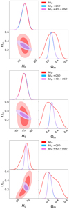 |
Fig. 1. Two-dimensional plots and 1D marginalized distributions with 1σ and 2σ contours of cosmological parameters (H0 and Ωm) in the framework of flat ΛCDM (upper), flat PEDE (lower left), and flat DGP (lower right) models with lensed quasars (6DΔt, 4Dd) and radio quasars (QSOs). |
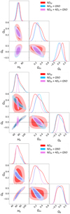 |
Fig. 2. Two-dimensional plots and 1D marginalized distributions with 1σ and 2σ contours of cosmological parameters (H0, Ωm, and Ωk) in the framework of non-flat ΛCDM (upper), non-flat PEDE (lower left), and non-flat DGP (lower right) models with lensed quasars (6DΔt, 4Dd) and unlensed quasars (QSOs). |
Best-fit values and 1σ uncertainties for the parameters H0, Ωm, Ωrc (if available), and Ωk in each cosmological model and quasar data set.
Flat cases. The constraint results for the three flat cosmological models are presented in Fig. 1, where we show the 2D confidence regions (with 1σ and 2σ limits) as well as 1D marginalized distributions from different data combinations. Our findings show that the constraints we obtain from the combination of the latest observations of quasars are more reliable than those derived from the independent quasar sample. Fortunately, the results in Fig. 2 show that the radio quasar data place remarkable constraints on all the parameters of the three cosmological models, and the degeneracy among different model parameters is broken. When combined with the data from the 120 unlensed quasars, the 6 time-delay lensed quasars would produce tighter constraints on the matter density parameter in all three cosmological scenarios. The measured Ωm ranges from a low value of  (flat DGP) to a high value of
  (flat PEDE). In particular, for flat ΛCDM the derived matter density parameter from the 120 unlensed quasars and 6 time-delay lensed quasars
  shows a perfect agreement with the TT, TE, EE+lowE+lensing results of Planck Collaboration (Ωm = 0.3103 ± 0.0057) (Planck Collaboration VI 2020). These findings are different from those obtained from the latest compilation of X-ray+UV quasars acting as standard candles, which favor a higher value of the matter density parameter at higher redshifts (Risaliti & Lusso 2019; see also Lian et al. 2021 for further discussion of this issue). In spite of the low mean values of Ωm in the flat DGP model, the constraints on Ωm obtained with the 6DΔt, 6DΔt+QSO, and 6DΔt+QSO+4Dd data are consistent with those obtained from other astrophysical probes (Xu & Wang 2010; Xu 2014; Giannantonio et al. 2008). For comparison, the corresponding fits on the parameter of Ωrc in flat DGP model are also displayed in Table 1. Finally, our analysis demonstrates that the matter density parameter plays an important role in the determination of the Hubble constant, which can be clearly seen from the anticorrelation between Ωm and H0 in Fig. 1.
The constraints on the Hubble constant are between  (DGP) and
  (PEDE) with six time-delay lensed quasars, which shift to
  (DGP) and
  (PEDE) with the combined 6DΔt+QSO data. Specifically, for the flat ΛCDM and PEDE models the mean values of H0 obtained with 6DΔt+4Dd+QSO data are more consistent with the recent determinations of H0 from the Supernovae H0 for the SH0ES collaboration (Riess et al. 2019). However, in the framework of the flat DGP model, the measured value of H0 with 1σ uncertainty (
 ), which is 3.6σ lower than the statistical estimates of the SH0ES results, demonstrates a perfect agreement with that derived from the recent Plank CMB observations (Planck Collaboration VI 2020). In addition, relative to the 6DΔt+QSO constraints, the Hubble constant derived from the combined 6DΔt+4DL+QSO data are a little higher than those values measured from the 6DΔt+QSO case. However, these differences are not statistically significant given the error bars, as can be seen from the numerical results summarized in Table 1.
Non-flat cases. As was revealed in the recent studies of (Di Valentino et al. 2020, 2021; Handley 2021), the discrepancy between the Hubble constant and cosmic curvature measured locally and inferred from Planck highlights the importance of considering non-flat cosmological models in this work. The constraint results for the three flat cosmological models are presented in Fig. 2, where we show the 2D confidence regions (with 1σ and 2σ limits) as well as 1D marginalized distributions from different data combinations. The numerical results are also summarized in Table 1. The upper panel of Fig. 2 shows that, in the concordance ΛCDM cosmology, a stringent constraint on the Hubble constant could be obtained from six time-delay quasar data DΔt ( ). However, the MCMC chains failed to converge for the other two model parameters, the matter density and cosmic curvature parameters (Ωm, Ωk). This issue could be appropriately addressed with stringent constraints produced by the combination of 120 QSO sample and 6 time-delay lensed quasars, with the best-fitting values at 68.3% confidence level for the three parameters:
  ,
,  , and
, and  . With the combined data sets 6DΔt+QSO+4Dd, we also obtain stringent constraints on the model parameters
  ,
,  , and
, and  . Compared with the previous results obtained in other model-independent methods (Qi et al. 2019b), our analysis results demonstrate that the strong degeneracy between the Hubble constant, the matter density parameter, and the cosmic curvature would be effectively broken by the combination of the latest observations of quasars (i.e., the angular size of compact structure in radio quasars and the time delays from gravitationally lensed quasars). The combination of the quasar data sets, justified by their consistency within 1σ, retains the same correlation between H0 and Ωk as distinct samples of quasars. For the determination of the Hubble constant, our constraint in the framework of non-flat ΛCDM cosmology is consistent with the local Hubble constant measurement from the SH0ES collaboration (Riess et al. 2019). The determination of Ωk suggests no significant deviation from flat spatial hypersurfaces, although favoring a somewhat positive value in the non-flat ΛCDM case.
In the case of the non-flat PEDE model it can be clearly seen from the comparison plots presented in Fig. 2 that there is a consistency between 6DΔt, 6DΔt+QSO, and 6DΔt+4Dd+QSO data sets. Our results confirm that the combination of compact structure in radio quasars and angular diameter distances to the lenses (4Dd) could break the degeneracy between the cosmological parameters and lead to more stringent constraints on all of the cosmological parameters, which is the most unambiguous result of the current lensed+unlensed quasar data set. Interestingly, the 6DΔt+QSO data generate a higher matter density parameter  than the other quasar samples (
 for 6DΔt and
  for 6DΔt+4Dd+QSO). For the Hubble constant inferred from the 6DΔt, 6DΔt+QSO, and 6DΔt+4Dd+QSO data sets, it is clear that the combination of 6DΔt with 120 unlensed quasar data points will result in a lower H0, but adding 4Dd data to the combination would increase the median value of H0 comparing to the H0 values obtained from 6DΔt alone. The estimated values of the Hubble constant in the non-flat PEDE model are between
  and
and  with 6DΔt and 6DΔt+4Dd+QSO data, which in broad terms agree very well with the standard values reported by the SH0ES collaboration (Riess et al. 2019). For the determination of cosmic curvature in the non-flat PEDE model, our results show that there is no significant evidence indicating its deviation from zero (spatially flat geometry). More specifically, the two quasar samples of 6DΔt and 6DΔt+QSO favor closed geometry (
 ,
,  ), while an open universe is favored by the 6DΔt+4Dd+QSO data sets with
  .
.
Finally, we perform a comparative analysis of the current lensed+unlensed quasar data set in the non-flat DGP model. The 1σ and 2σ confidence level contours for the parameter estimations are shown in Fig. 2, with the marginalized best-fitting parameters and 1σ uncertainties summarized in Table 1. We note that for such a modified gravity model (i.e., the gravity arising from the braneworld theory), the best-fitting matter density parameter will be considerably shifted to a lower value. Our final assessments of the matter density with the corresponding 1σ uncertainties ( ,
,  , and
, and  with the 6DΔt, 6DΔt+QSO, and 6DΔt+4Dd+QSO data sets) are consistent with the standard values reported by other astrophysical probes, such as growth factors combined with CMB+BAO+SNe Ia observations (Xia 2009), Hubble parameters combined with CMB+SNe Ia data (Fang et al. 2008), statistical analysis of strong gravitational lensing systems (Cao et al. 2011b, 2012b; Ma et al. 2019; Liu et al. 2020b), and the observations of compact structure in intermediate-luminosity radio quasars (Cao et al. 2017; Liu et al. 2019, 2021b). For comparison, the corresponding fits on the parameter of Ωrc are also displayed in Table 1. We note here that the DGP model reduces to the concordance ΛCDM model when Ωrc = 0. Considering its nonvanishing value revealed in this analysis and previous works (Ωrc ∼ 0.14), our fitting result shows the DGP model fails to recover and is only a bit worse than the ΛCDM under the current observational tests (see also Fang et al. 2008; Cao et al. 2011b). We also investigate how sensitive our results on H0 and Ωk are regarding the choice of this cosmological model. On the one hand, the measured value of H0 with 1σ uncertainty derived from the latest quasar sample,
  (6DΔt) and
  (6DΔt+QSO), shows a perfect consistency with that derived from the recent Planck CMB observation (Planck Collaboration VI 2020). On the other hand, our final assessments of the cosmic curvature with corresponding 1σ uncertainty are
  and
and  with the two quasar samples (6DΔt and 6DΔt+QSO), which are more consistent with flat spatial hypersurfaces than with the value found by Qi et al. (2019b). From the joint analysis with lensed+unlensed quasar data, we find that the Hubble constant and the spatial curvature parameter are constrained to be
  and
and  , which further confirms the above conclusions.
We now discuss the H0 and Ωk measurements from the newly compiled sample of ultra-compact structure in radio quasars and strong gravitational lensing systems with quasars acting as background sources. The H0 determination from six spatially flat and non-flat cosmological models (ΛCDM, PEDE, and DGP) are displayed in Fig. 3. A joint analysis of the quasar sample (the time-delay measurements of six strong lensing systems, four angular diameter distances to the lenses, and 120 intermediate-luminosity quasars calibrated as standard rulers) provides model-independent estimations of the Hubble constant H0, which is strongly consistent with that derived from the local distance ladder by the SH0ES collaboration in the ΛCDM and PEDE model. However, in the framework of a DGP cosmology (especially for the flat universe), the measured Hubble constant is in good agreement with that derived from the recent Planck 2018 results. Meanwhile, our results also demonstrate that zero spatial curvature is supported by the current lensed and unlensed quasar observations and there is no significant deviation from a flat universe. Finally, our results provide independent evidence for the accelerated expansion of the Universe, with the existence of dominant dark energy density (Ωm ∼ 0.30) in the framework of six cosmologies classified into different categories. This is the most unambiguous result of the current quasar data sets.
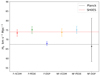 |
Fig. 3. Determination of Hubble constant from the combined data of lensed quasars (6DΔt and 4Dd) and unlensed radio quasars (QSOs), in the framework of six spatially flat (F) and non-flat (NF) cosmological models (ΛCDM, PEDE, and DGP). |
Model comparison. The values of DIC for all models are reported in Table 1. According to the number of model parameters, these six cosmological models can be divided into two classes: the two-parameter models (including the flat ΛCDM, flat PEDE, and flat DGP) and the three-parameter models (including non-flat ΛCDM, non-flat PEDE, and non-flat DGP). For the two-parameter models, the flat PEDE provides the smallest information criterion result (DIC = 390.68) of all the flat cosmological models. However, we note that the difference in DIC between the flat PEDE and flat ΛCDM model is only ΔDIC = 0.65, which means these two models are comparable to each other according to this criterion. The flat DGP model is the worst one to explain the current lensed and unlensed quasar observations, since the DIC value it yields is the largest of the two-parameter models (ΔDIC = 2.99). As for the three-parameter models, the DIC results show that the non-flat ΛCDM model is still not the best one. The non-flat PEDE model, which is a little bit better than the non-flat ΛCDM, performs best in explaining the quasar data (DIC = 393.45), with positive evidence against non-flat DGP (ΔDIC = 1.82).
We also provide a graphical representation of the DIC results in Fig. 4 that directly shows the results of the IC test for each model. Out of all the candidate models, it is obvious that the flat PEDE and flat ΛCDM are the two most favored models in the data combination of lensed+unlensed quasars. Next are the flat DGP, non-flat ΛCDM, and non-flat PEDE, which give comparable fits to the data. According to the DIC results, the most disfavored model is non-flat DGP, with strong evidence against the cosmological scenario among the six models we study here.
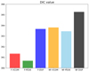 |
Fig. 4. Graphical representation of the DIC values for six spatially flat (F) and non-flat (NF) cosmological models (ΛCDM, PEDE, and DGP), based on the combined data of lensed quasars (6DΔt and 4Dd) and unlensed radio quasars (QSOs). |
5. Conclusions
In this paper we analyzed six spatially flat and non-flat cosmological models (ΛCDM, PEDE, and DGP) using a newly compiled sample of ultra-compact structure in radio quasars and strong gravitational lensing systems with quasars acting as background sources. This study is strongly motivated by the need to revisit the Hubble constant, spatial curvature, and dark energy dynamics in the framework of different cosmological models of interests, and to search for the implications for the non-flat Universe and extensions of the standard cosmological model (the spatially flat ΛCDM). The inclusion of such a newly compiled quasar sample in the cosmological analysis is crucial to this aim as it will extend the Hubble diagram to a high-redshift range in which predictions from different cosmological models can be distinguished (Capozziello et al. 2006). From the constraints derived using the updated observations of quasars, we can identify some relatively model-independent features.
In all the cosmological models, the cosmological parameters obtained from distinct quasar samples are consistent and the combination of the latest observations of quasars (i.e., the time-delay measurements of six strong lensing systems, four angular diameter distances to the lenses, and 120 intermediate-luminosity quasars calibrated as standard rulers) would break the degeneracy between the Hubble constant and other cosmological parameters. The lensed quasar (6DΔt and 4Dd) and unlensed radio quasar (QSO) data combination produces the most reliable constraints. In particular, for most of the cosmological models we studied here (flat ΛCDM, non-flat ΛCDM, flat PEDE, and non-flat PEDE), the derived matter density parameter is completely consistent with Ωm ∼ 0.30 in all the data sets, as expected from the latest cosmological observations (Wong et al. 2020; Cao et al. 2017, 2020; Liu et al. 2019; Li et al. 2017; Lian et al. 2021) and Planck Collaboration results (Ωm = 0.3103 ± 0.0057) (Planck Collaboration VI 2020). Nevertheless, the DGP model in both flat and non-flat cases shows a deviation from this prediction, with statistically lower values of  and
and  for the combined sample of 6DΔt+4Dd+QSO. A joint analysis of the quasar sample provides model-independent estimations of the Hubble constant H0, which is strongly consistent with that derived from the local distance ladder by SH0ES collaboration (Riess et al. 2019) in the ΛCDM and PEDE model. However, in the framework of a DGP cosmology (especially for the flat universe), the measured value of H0 with 1σ uncertainty, which is 3.6σ lower than the statistical estimates of the SH0ES results, demonstrates a perfect agreement with that derived from the recent Plank CMB observations (Planck Collaboration VI 2020). Our findings also confirm the flatness of our universe (Collett et al. 2019; Wei & Melia 2020; Qi et al. 2021), which is the most unambiguous result of the current lensed and unlensed quasar observations, although there is some room for a little spatial curvature energy density in the non-flat ΛCDM, non-flat PEDE, and non-flat DGP cases. Finally, we statistically evaluate which model is more consistent with the observational quasar data. Concerning the ranking of competing dark energy models, the flat PEDE is the most favored of all the candidate models, while the non-flat DGP is substantially penalized by the DIC criteria. However, our analysis still does not rule out dark energy being a cosmological constant or non-flat spatial hypersurfaces.
Considering the possible controversy around the systematics of the observed angular sizes of compact radio quasars (Kellermann 1993), the other reasonable strategy to quantify this effect of the systematics is taking σsys as an additional free parameter, which should be fitted simultaneously with the cosmological parameters of interest. This strategy was extensively applied in the derivation of quasar distances based on the nonlinear relation between their UV and X-ray fluxes, based on the largest quasar sample consisting of 12 000 objects with both X-ray and UV observations (Risaliti & Lusso 2019). In this paper we performed a sensitivity analysis by introducing an overall 5% and 20% systematical uncertainty to the angular size measurements of compact radio quasars in order to investigate how the cosmological constraints on flat PEDE is altered by different choices of systematics. In the framework of such an error strategy in the construction of posterior likelihood ℒQSO, the matter density parameter and Hubble constant respectively change to  ,
,  (5% systematical uncertainty), and
  ,
,  (20% systematical uncertainty). The comparison of the resulting constraints on Ωm and H0 based on different systematical uncertainties is shown in Fig. 5. In general, it is easy to check that the derived value of Ωm is more sensitive to the systematical uncertainties of angular size measurements; in other words, larger systematic uncertainties will shift the matter density parameter to a higher value. This illustrates the importance of a larger quasar sample from future VLBI observations based on better UV coverage (Pushkarev & Kovalev 2015). As a final remark, from the observational point of view, we can see that the 120 unlensed radio quasars have perfect coverage of source redshifts in six strong lensing systems (z ∼ 3). Given the usefulness of compact radio quasars and strongly lensed quasars acting as standard rulers at high redshifts, we pin our hopes on a large amount of intermediate-luminosity radio quasars detected by future VLBI surveys at different frequencies (Pushkarev & Kovalev 2015), and strongly lensed quasars with well-measured time delays discovered by future surveys of the Large Synoptic Survey Telescope (Collett 2015).
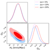 |
Fig. 5. Cosmological constraints on the flat PEDE model from the combined quasar data, with different systematical uncertainties in the angular size measurements of unlensed radio quasars (QSOs). |
Acknowledgments
This work was supported by the National Natural Science Foundation of China under Grants Nos. 12203009, 12021003, 11690023, 11920101003; the Strategic Priority Research Program of the Chinese Academy of Sciences, Grant No. XDB23000000; the Interdiscipline Research Funds of Beijing Normal University; and the China Manned Space Project (Nos. CMS-CSST-2021-B01 and CMS-CSST-2021-A01). X. Li was supported by National Natural Science Foundation of China under Grants No. 1200300, Hebei NSF under Grant No. A2020205002 and the fund of Hebei Normal University under Grants No. L2020B02.
References
- Alam, U., Bag, S., & Sahni, V. 2017, Phys. Rev. D, 95, 023524 [NASA ADS] [CrossRef] [Google Scholar]
- Bag, S., Shafieloo, A., Liao, K., et al. 2022, ApJ, 927, 191 [NASA ADS] [CrossRef] [Google Scholar]
- Birrer, S., Amara, A., & Refregier, A. 2016, JCAP, 2016, 020 [CrossRef] [Google Scholar]
- Birrer, S., Treu, T., Rusu, C. E., et al. 2019, MNRAS, 484, 4726 [Google Scholar]
- Briffa, R., Capozziello, S., Said, J. L., et al. 2020, CQG, 38, 055007 [NASA ADS] [CrossRef] [Google Scholar]
- Caldera-Cabral, G., Maartens, R., & Ureña-López, L. A. 2009, Phys. Rev. D, 79, 063518 [NASA ADS] [CrossRef] [Google Scholar]
- Cao, S., & Zhu, Z.-H. 2014, Phys. Rev. D, 90, 083006 [NASA ADS] [CrossRef] [Google Scholar]
- Cao, S., Liang, N., & Zhu, Z.-H. 2011a, MNRAS, 416, 1099 [NASA ADS] [CrossRef] [Google Scholar]
- Cao, S., Zhu, Z.-H., & Zhao, R. 2011b, Phys. Rev. D, 84, 023005 [NASA ADS] [CrossRef] [Google Scholar]
- Cao, S., Pan, Y., Biesiada, M., et al. 2012a, JCAP, 2012, 016 [CrossRef] [Google Scholar]
- Cao, S., Covone, G., & Zhu, Z.-H. 2012b, ApJ, 755, 31 [NASA ADS] [CrossRef] [Google Scholar]
- Cao, S., Biesiada, M., Gavazzi, R., et al. 2015, ApJ, 806, 185 [NASA ADS] [CrossRef] [Google Scholar]
- Cao, S., Zheng, X., Biesiada, M., et al. 2017, A&A, 606, A15 [NASA ADS] [CrossRef] [EDP Sciences] [Google Scholar]
- Cao, S., Biesiada, M., Qi, J., et al. 2018, Eur. Phys. J. C, 78, 749 [NASA ADS] [CrossRef] [Google Scholar]
- Cao, S., Qi, J., Biesiada, M., et al. 2019, Phys. Dark Universe, 24, 100274 [NASA ADS] [CrossRef] [Google Scholar]
- Cao, S., Ryan, J., & Ratra, B. 2020, MNRAS, 497, 3191 [NASA ADS] [CrossRef] [Google Scholar]
- Capozziello, S., Cardone, V. F., & Troisi, A. 2006, JCAP, 2006, 001 [CrossRef] [Google Scholar]
- Chen, G. C.-F., Fassnacht, C. D., Suyu, S. H., et al. 2019, MNRAS, 490, 1743 [NASA ADS] [CrossRef] [Google Scholar]
- Collett, T. E. 2015, ApJ, 811, 20 [NASA ADS] [CrossRef] [Google Scholar]
- Collett, T., Montanari, F., & Räsänen, S. 2019, Phys. Rev. Lett., 123, 231101 [CrossRef] [Google Scholar]
- Deffayet, C., Dvali, G., & Gabadadze, G. 2002a, Phys. Rev. D, 65, 044023 [NASA ADS] [CrossRef] [Google Scholar]
- Deffayet, C., Landau, S. J., Raux, J., et al. 2002b, Phys. Rev. D, 66, 024019 [CrossRef] [Google Scholar]
- Di Valentino, E., Melchiorri, A., Fantaye, Y., et al. 2018, Phys. Rev. D, 98, 063508 [NASA ADS] [CrossRef] [Google Scholar]
- Di Valentino, E., Melchiorri, A., & Silk, J. 2020, Nat. Astron., 4, 196 [Google Scholar]
- Di Valentino, E., Melchiorri, A., & Silk, J. 2021, ApJ, 908, L9 [NASA ADS] [CrossRef] [Google Scholar]
- Ding, X., Treu, T., Birrer, S., et al. 2021, MNRAS, 503, 1096 [Google Scholar]
- Dvali, G., Gabadadze, G., & Porrati, M. 2000, Phys. Lett. B, 485, 208 [Google Scholar]
- Dvali, G., Gabadadze, G., & Shifman, M. 2001, Phys. Lett. B, 497, 271 [NASA ADS] [CrossRef] [Google Scholar]
- Fang, W., Wang, S., Hu, W., et al. 2008, Phys. Rev. D, 78, 103509 [NASA ADS] [CrossRef] [Google Scholar]
- Follin, B., & Knox, L. 2018, MNRAS, 477, 4534 [NASA ADS] [CrossRef] [Google Scholar]
- Foreman-Mackey, D., Hogg, D. W., Lang, D., et al. 2013, PASP, 125, 306 [NASA ADS] [CrossRef] [Google Scholar]
- Giannantonio, T., Song, Y.-S., & Koyama, K. 2008, Phys. Rev. D, 78, 044017 [NASA ADS] [CrossRef] [Google Scholar]
- Handley, W. 2021, Phys. Rev. D, 103, L041301 [NASA ADS] [CrossRef] [Google Scholar]
- Hashim, M., El Hanafy, W., Golovnev, A., et al. 2021a, JCAP, 2021, 052 [CrossRef] [Google Scholar]
- Hashim, M., El-Zant, A. A., El Hanafy, W., et al. 2021b, JCAP, 2021, 053 [CrossRef] [Google Scholar]
- Jee, I., Komatsu, E., Suyu, S. H., et al. 2016, JCAP, 2016, 031 [Google Scholar]
- Jee, I., Suyu, S. H., Komatsu, E., et al. 2019, Science, 365, 1134 [NASA ADS] [CrossRef] [Google Scholar]
- Jiménez Cruz, N. M., & Escamilla-Rivera, C. 2021, Eur. Phys. J. Plus, 136, 51 [CrossRef] [Google Scholar]
- Koyama, K. 2016, Rep. Prog. Phys., 79, 046902 [NASA ADS] [CrossRef] [Google Scholar]
- Karwal, T., & Kamionkowski, M. 2016, Phys. Rev. D, 94, 103523 [NASA ADS] [CrossRef] [Google Scholar]
- Kellermann, K. I. 1993, Nature, 361, 134 [NASA ADS] [CrossRef] [Google Scholar]
- Li, X., & Shafieloo, A. 2019, ApJ, 883, L3 [NASA ADS] [CrossRef] [Google Scholar]
- Li, X., & Shafieloo, A. 2020, ApJ, 902, 58 [NASA ADS] [CrossRef] [Google Scholar]
- Li, X., Cao, S., Zheng, X., et al. 2017, ArXiv e-prints [arXiv:1708.08867] [Google Scholar]
- Li, X., Shafieloo, A., Sahni, V., et al. 2019, ApJ, 887, 153 [NASA ADS] [CrossRef] [Google Scholar]
- Liao, K. 2021, ApJ, 906, 26 [NASA ADS] [CrossRef] [Google Scholar]
- Liao, K., Shafieloo, A., Keeley, R. E., et al. 2019, ApJ, 886, L23 [NASA ADS] [CrossRef] [Google Scholar]
- Liao, K., Shafieloo, A., Keeley, R. E., et al. 2020, ApJ, 895, L29 [NASA ADS] [CrossRef] [Google Scholar]
- Lian, Y., Cao, S., Biesiada, M., et al. 2021, MNRAS, 505, 2111 [NASA ADS] [CrossRef] [Google Scholar]
- Liu, T., Cao, S., Zhang, J., et al. 2019, ApJ, 886, 94 [NASA ADS] [CrossRef] [Google Scholar]
- Liu, T., Cao, S., Biesiada, M., et al. 2020a, ApJ, 899, 71 [NASA ADS] [CrossRef] [Google Scholar]
- Liu, T., Cao, S., Zhang, J., et al. 2020b, MNRAS, 496, 708 [NASA ADS] [CrossRef] [Google Scholar]
- Liu, T., Cao, S., Zhang, S., et al. 2021a, Eur. Phys. J. C, 81, 903 [NASA ADS] [CrossRef] [Google Scholar]
- Liu, T., Cao, S., Biesiada, M., et al. 2021b, MNRAS, 506, 2181 [NASA ADS] [CrossRef] [Google Scholar]
- Liddle, A. R. 2007, MNRAS, 377, L74 [NASA ADS] [Google Scholar]
- Lyu, M.-Z., Haridasu, B. S., Viel, M., et al. 2020, ApJ, 900, 160 [NASA ADS] [CrossRef] [Google Scholar]
- Ma, Y., Zhang, J., Cao, S., et al. 2017, Eur. Phys. J. C, 77, 891 [NASA ADS] [CrossRef] [Google Scholar]
- Ma, Y.-B., Cao, S., Zhang, J., et al. 2019, Eur. Phys. J. C, 79, 121 [NASA ADS] [CrossRef] [Google Scholar]
- Melia, F. 2018, Europhys. Lett., 123, 39001 [NASA ADS] [CrossRef] [Google Scholar]
- Multamäki, T., Gaztañaga, E., & Manera, M. 2003, MNRAS, 344, 761 [CrossRef] [Google Scholar]
- Perlick, V. 1990a, CQG, 7, 1319 [NASA ADS] [CrossRef] [Google Scholar]
- Perlick, V. 1990b, CQG, 7, 1849 [NASA ADS] [CrossRef] [Google Scholar]
- Perivolaropoulos, L., & Skara, F. 2021, Phys. Rev. D, 104, 123511 [NASA ADS] [CrossRef] [Google Scholar]
- Planck Collaboration XIII. 2016, A&A, 594, A13 [NASA ADS] [CrossRef] [EDP Sciences] [Google Scholar]
- Planck Collaboration VI. 2020, A&A, 641, A6 [NASA ADS] [CrossRef] [EDP Sciences] [Google Scholar]
- Pushkarev, A. B., & Kovalev, Y. Y. 2015, MNRAS, 452, 4274 [NASA ADS] [CrossRef] [Google Scholar]
- Qi, J.-Z., Cao, S., Biesiada, M., et al. 2017, Eur. Phys. J. C, 77, 502 [NASA ADS] [CrossRef] [Google Scholar]
- Qi, J., Cao, S., Biesiada, M., et al. 2019a, Phys. Rev. D, 100, 023530 [NASA ADS] [CrossRef] [Google Scholar]
- Qi, J.-Z., Cao, S., Zhang, S., et al. 2019b, MNRAS, 483, 1104 [NASA ADS] [CrossRef] [Google Scholar]
- Qi, J.-Z., Zhao, J.-W., Cao, S., et al. 2021, MNRAS, 503, 2179 [NASA ADS] [CrossRef] [Google Scholar]
- Rathna Kumar, S., Stalin, C. S., & Prabhu, T. P. 2015, A&A, 580, A38 [NASA ADS] [CrossRef] [EDP Sciences] [Google Scholar]
- Ren, X., Wong, T. H. T., Cai, Y.-F., et al. 2021, Phys. Dark Universe, 32, 10081 [Google Scholar]
- Riess, A. G., Strolger, L.-G., Casertano, S., et al. 2007, ApJ, 659, 98 [NASA ADS] [CrossRef] [Google Scholar]
- Riess, A. G., Casertano, S., Yuan, W., et al. 2019, ApJ, 876, 85 [Google Scholar]
- Risaliti, G., & Lusso, E. 2019, Nat. Astron., 3, 272 [Google Scholar]
- Ryan, J. 2021, JCAP, 2021, 051 [CrossRef] [Google Scholar]
- Rusu, C. E., Wong, K. C., Bonvin, V., et al. 2020, MNRAS, 498, 1440 [Google Scholar]
- Sonnenfeld, A. 2021, A&A, 656, A153 [NASA ADS] [CrossRef] [EDP Sciences] [Google Scholar]
- Spiegelhalter, D. J., Best, N. G., Carlin, B. P., & Van Der Linde, A. 2020, J. R. Stat. Soc. Ser. B (Stat. Methodol.), 64, 583 [Google Scholar]
- Suyu, S. H., Marshall, P. J., Auger, M. W., et al. 2010, ApJ, 711, 201 [Google Scholar]
- Suyu, S. H., Auger, M. W., Hilbert, S., et al. 2013, ApJ, 766, 70 [Google Scholar]
- Suyu, S. H., Treu, T., Hilbert, S., et al. 2014, ApJ, 788, L35 [NASA ADS] [CrossRef] [Google Scholar]
- Taubenberger, S., Suyu, S. H., Komatsu, E., et al. 2019, A&A, 628, L7 [NASA ADS] [CrossRef] [EDP Sciences] [Google Scholar]
- Treu, T., & Marshall, P. J. 2016, A&ARv, 24, 11 [Google Scholar]
- Väliviita, J., Maartens, R., & Majerotto, E. 2010, MNRAS, 402, 2355 [CrossRef] [Google Scholar]
- Vavryčuk, V., & Kroupa, P. 2020, MNRAS, 497, 378 [CrossRef] [Google Scholar]
- Wang, B., Qi, J.-Z., Zhang, J.-F., et al. 2020, ApJ, 898, 100 [NASA ADS] [CrossRef] [Google Scholar]
- Wei, J.-J., & Melia, F. 2020, ApJ, 897, 127 [NASA ADS] [CrossRef] [Google Scholar]
- Wong, K. C., Suyu, S. H., Auger, M. W., et al. 2017, MNRAS, 465, 4895 [NASA ADS] [CrossRef] [Google Scholar]
- Wong, K. C., Suyu, S. H., Chen, G. C.-F., et al. 2020, MNRAS, 498, 1420 [Google Scholar]
- Xia, J.-Q. 2009, Phys. Rev. D, 79, 103527 [NASA ADS] [CrossRef] [Google Scholar]
- Xu, L. 2014, JCAP, 2014, 048 [CrossRef] [Google Scholar]
- Xu, L., & Wang, Y. 2010, Phys. Rev. D, 82, 043503 [NASA ADS] [CrossRef] [Google Scholar]
- Yang, W., Pan, S., Vagnozzi, S., et al. 2019, JCAP, 2019, 044 [CrossRef] [Google Scholar]
- Zheng, X., Biesiada, M., Cao, S., et al. 2017, JCAP, 2017, 030 [Google Scholar]
All Tables
Best-fit values and 1σ uncertainties for the parameters H0, Ωm, Ωrc (if available), and Ωk in each cosmological model and quasar data set.
All Figures
|
Fig. 1. Two-dimensional plots and 1D marginalized distributions with 1σ and 2σ contours of cosmological parameters (H0 and Ωm) in the framework of flat ΛCDM (upper), flat PEDE (lower left), and flat DGP (lower right) models with lensed quasars (6DΔt, 4Dd) and radio quasars (QSOs). |
| In the text | |
|
Fig. 2. Two-dimensional plots and 1D marginalized distributions with 1σ and 2σ contours of cosmological parameters (H0, Ωm, and Ωk) in the framework of non-flat ΛCDM (upper), non-flat PEDE (lower left), and non-flat DGP (lower right) models with lensed quasars (6DΔt, 4Dd) and unlensed quasars (QSOs). |
| In the text | |
|
Fig. 3. Determination of Hubble constant from the combined data of lensed quasars (6DΔt and 4Dd) and unlensed radio quasars (QSOs), in the framework of six spatially flat (F) and non-flat (NF) cosmological models (ΛCDM, PEDE, and DGP). |
| In the text | |
|
Fig. 4. Graphical representation of the DIC values for six spatially flat (F) and non-flat (NF) cosmological models (ΛCDM, PEDE, and DGP), based on the combined data of lensed quasars (6DΔt and 4Dd) and unlensed radio quasars (QSOs). |
| In the text | |
|
Fig. 5. Cosmological constraints on the flat PEDE model from the combined quasar data, with different systematical uncertainties in the angular size measurements of unlensed radio quasars (QSOs). |
| In the text | |
Current usage metrics show cumulative count of Article Views (full-text article views including HTML views, PDF and ePub downloads, according to the available data) and Abstracts Views on Vision4Press platform.
Data correspond to usage on the plateform after 2015. The current usage metrics is available 48-96 hours after online publication and is updated daily on week days.
Initial download of the metrics may take a while.