© ESO 2020

1. Introduction

The dynamics close to the Lagrangian points L₁ and L₂ of the Sun–Earth circular restricted three-body problem (CR3BP) have been extensively discussed in recent decades in connection with space-mission design (the reader is referred to Martin et al. 2010; van Damme et al. 2010; Koon et al. 2006; Parker & Anderson 2013; Gómez et al. 2004, and references therein for further information). ISEE-3, SOHO, WMAP, Genesis, Herschel and Planck are just few examples of missions in which the spacecraft reached the vicinity of the L₁ and L₂ Lagrangian points of the Sun–Earth system during its journey. While L₃ is also potentially useful for astrodynamics (Gómez et al. 2001; Gómez & Mondelo 2001; Barrabés & Ollè 2006; Terra et al. 2014; Pàez & Efthymiopoulos 2015; Jorba & Nicolás 2020), no significant attention has been paid to the Sun–Earth L₃ point even if its Lyapunov orbits have been proposed as an ideal place for spacecraft because of the possibility to obtain data for the Sun, the inner planets, and the main belt from a new perspective (Hou et al. 2007; Tantardini et al. 2010). The aim of this study is to find orbits close to the Sun–Earth L₃ point that are useful for applications of astrodynamics. In particular, this refers to orbits that remain close to L₃ within useful distances at least for several decades in a model of the Solar System whose ephemerides are comparable with those provided by the JPL computation service. Because the planetary perturbations on the Sun–Earth Lagrangian point L₃ are stronger than Earth’s attraction itself, the CR3BP is not a realistic approximation of the dynamics close to L₃. The main differences between the real Solar System and the Sun–Earth circular restricted problem are caused by the planetary perturbations (mainly from Venus and Jupiter) and in the elliptic orbit of the Earth. To quantify the effects of planetary perturbations, we first consider a multicircular restricted problem (MCR8BP), where the eight planets of our Solar System (from Mercury to Neptune) perform circular motions around the Sun. Using Hamiltonian perturbation theory we find that the Hamiltonian of the MCR8BP is conjugate by a canonical transformation to an averaged Hamiltonian system that still has an equilibrium point close to L₃ (within terms of second order in the planetary masses and fourth order in eccentricity). This equilibrium, which we denote by ℒ₃, is aligned in the Sun–Earth direction. The individual contribution of each planet to the displacement of ℒ₃ from L₃ is reported in the first column of Table 1. It is remarkable that while Venus and Jupiter each move the position of this equilibrium by about 218 and 176 km, respectively, in opposite directions, in the model where both planets are included, their effects almost perfectly compensate for one another, leaving a displacement of about 40 km only (the contributions of the other planets being smaller by about two orders of magnitude). The equilibrium ℒ₃ is then mapped in the original system to a quasi-periodic dynamical substitute; the contributions of each planet to the amplitude of this quasi-periodic libration around L₃, which are reported in the second column of Table 1, are quite large and sum to about d = 10⁻⁴ AU ∼15 000 km. Since the linear stability of ℒ₃ is the same as that of L₃, the averaged Hamiltonian, approximated within terms of second order in the planetary masses, has close to ℒ₃ a dynamics similar to that of L₃ in the CR3BP; this means that in the vicinity of ℒ₃ there are periodic and quasi-periodic orbits. The image of these orbits in the original MCR8BP provides orbits librating around L₃ of amplitudes larger than the amplitude of the dynamical substitute, which we denote hereafter by d. Since the MCR8BP is still a rough approximation of the real Solar System, we use fast Lyapunov indicators (FLI) to look for orbits of this kind in a model of the Solar System that is compatible with the precision of JPL digital ephemerides. In the last decade, the FLI have been used to find orbits related to the dynamics close to the Lagrangian points of the restricted three-body problem (Lega et al. 2011; Guzzo & Lega 2013, 2014, 2018) and to close encounters in cometary dynamics (Guzzo & Lega 2013, 2017). The method provides orbits that remain, within a given time-span, in a neighborhood ℬ of the dynamical substitute obtained from an approximated model. In order to construct the neighborhood ℬ, we must also consider the differences between the real Solar System and the Sun–Earth CR3BP caused by the elliptic orbit of the Earth. The CR3BP is traditionally compared to the elliptic restricted three-body problem (ER3BP) by introducing a rotating-pulsating Cartesian reference frame $O\widehat{X}\widehat{Y}\widehat{Z}$ in which the primary and the secondary bodies remain in fixed locations of the $\widehat{X}$ axis (see e.g., Szebehely 1967). More precisely however, in the rotating-pulsating reference frame the ER3BP still has the Lagrange equilibria in the same positions as the circular problem. We therefore proceed as follows: for any given libration amplitude α >  d, we first compute a Lyapunov orbit of the CR3BP of amplitude α, hereafter referred to as the planar Lyapunov orbit. We use this orbit as an input of the FLI method to find orbits of the ER3BP that, in the pulsating frame, remain close to the previous Lyapunov orbit for up to 200 years. We then consider the motions of the Sun and the Earth in the realistic model of the Solar System, and we introduce a new rotating-pulsating reference frame OXYZ in which the Sun and the Earth remain in fixed locations of the X axis, and we map the previous orbit to this reference frame. Finally, since the planetary perturbations introduce oscillations of amplitude d, we define the set ℬ as a neighborhood of the previous orbit of amplitude ρ ∈ (d, α/10), and we find orbits of the realistic model of the Solar System which remain in the set ℬ for a minimum of 200 years. For α <  10d, we apply the method using a ball ℬ centered at ℒ₃ of radius α. For the minimum value of α = 2d we find an orbit stable up to 250 years in a neighborhood of ℒ₃. As an illustration of our method, we reproduce a sample of these orbits in Figs. 4 and 7.

The paper is organized as follows: in Sect. 2 we introduce the MCR8BP and we study the system obtained by averaging the mean anomalies of the planets (except for the Earth); in particular, we introduce ℒ₃ and compute the dynamical substitute in the original system conjugate to such equilibrium. In Sect. 3 we define the FLI method allowing us to recover orbits that remain in the neighborhood of L₃ for at least 200 years in a model of the Solar System that is compatible with the JPL ephemerides.

2. The planar multicircular restricted planetary problem

2.1. Equations of motion

Let us consider the simplified planar model MCR8BP of our Solar System, where the eight planets from Mercury to Neptune perform circular motions around a fixed Sun in the same orbital plane. Our aim is to study the dynamics of a spacecraft gravitationally attracted by the planets close to the Sun–Earth Lagrangian equilibrium point L₃. We use μ and ε_j to denote the gravitational parameters of the Sun and of the j-th planet, respectively, and n_j the mean motion of the j-th planet. In an inertial reference frame Oxy centered at the Sun, the j-th planet position is identified by r_j(t) = d_j (cos (n_jt + ϕ_j), sin (n_jt + ϕ_j)), where d_j and ϕ_j denote the orbital radius and the initial value of the mean anomalies respectively. In order to compare the dynamics of the system with the dynamics of the Sun–Earth CR3BP we define the Hamiltonian of the system in a reference frame OXY centered at the Sun and such that the Earth position is (d₃, 0):

$$\begin{array}{c}\hfill \begin{array}{cc}\hfill H(P_X,P_Y,X,Y;t)& =H_0(P_X,P_Y,X,Y)+{\epsilon }_3{H}_3(X,Y)\hfill \\ \hfill & +\sum _{j\ne 3}{\epsilon }_j{H}_j(X,Y;t)\hfill \end{array}\end{array}$$(1)

where

$$\begin{array}{cc}\hfill H_0& :=\frac{P_X^2+P_Y^2}{2}-n_3(X{P}_Y-Y{P}_X)-\frac{\mu }{\sqrt{X^2+Y^2}},\hfill \\ \hfill H_3& :=\frac{X}{d_3^2}-\frac{1}{\sqrt{{(X-d_3)}^2+Y^2}},\hfill \\ \hfill H_j& :=\frac{Xcos({\overline{n}}_{j}t+{\overline{\varphi }}_j)+Ysin({\overline{n}}_{j}t+{\overline{\varphi }}_j)}{d_j^2}-\hfill \\ \hfill & -\frac{1}{\sqrt{{(X-d_{j}cos({\overline{n}}_{j}t+{\overline{\varphi }}_j))}^2+{(Y-d_{j}sin({\overline{n}}_{j}t+{\overline{\varphi }}_j))}^2}},\hfill \end{array}$$

with j ≠ 3, where P_X and P_Y denote the momenta conjugate to X and Y, and ${\overline{n}}_j:=n_j-n_3$, ${\overline{\varphi }}_j:={\varphi }_j-{\varphi }_3$. We note that if ε_j = 0 for j  ≠  3, the Hamilton function (1) reduces to the Hamiltonian of the CR3BP; for this reason we treat ∑_j ≠ 3ε_jH_j(X, Y; t) as a quasi-periodic time-dependent perturbation of the Sun–Earth CR3BP.

2.2. Averaging the planetary anomalies

In this section we introduce a time-dependent near to the identity canonical transformation

$$\begin{array}{c}\hfill (P_X,P_Y,X,Y)=\mathcal{C}({\stackrel{\sim }{P}}_X,{\stackrel{\sim }{P}}_Y,\stackrel{\sim }{X},\stackrel{\sim }{Y};t),\end{array}$$

conjugating the Hamiltonian (1) to a Hamiltonian of the form

$$\begin{array}{c}\hfill \begin{array}{cc}\hfill \stackrel{\sim }{H}({\stackrel{\sim }{P}}_X,{\stackrel{\sim }{P}}_Y,\stackrel{\sim }{X},\stackrel{\sim }{Y};t)=& \overline{H}({\stackrel{\sim }{P}}_X,{\stackrel{\sim }{P}}_Y,\stackrel{\sim }{X},\stackrel{\sim }{Y})+\sum _{j\ne 3}{\mathcal{R}}_j^{\prime }({\stackrel{\sim }{P}}_X,{\stackrel{\sim }{P}}_Y,\stackrel{\sim }{X},\stackrel{\sim }{Y})\hfill \\ \hfill & +{\mathcal{R}}^{″}({\stackrel{\sim }{P}}_X,{\stackrel{\sim }{P}}_Y,\stackrel{\sim }{X},\stackrel{\sim }{Y};t),\hfill \end{array}\end{array}$$

where ${\mathcal{R}}_j^{\prime }$ is of first order in the planetary masses, fourth order in the eccentricity, and of order ${\epsilon }_j{\mathrm{\Delta }}_j^{36}$ where ${\mathrm{\Delta }}_j^{36}$ is defined as $\frac{1}{a}{\left(\frac{d_j}{a}\right)}^{36}$ for j <  3 and $\frac{1}{d_j}{\left(\frac{a}{d_j}\right)}^{36}$ for j >  3; ℛ″ is of second order in the planetary masses and

$$\begin{array}{c}\hfill \begin{array}{cc}\hfill \overline{H}({\stackrel{\sim }{P}}_X,{\stackrel{\sim }{P}}_Y,\stackrel{\sim }{X},\stackrel{\sim }{Y})& :=\frac{{\stackrel{\sim }{P}}_X^2+{\stackrel{\sim }{P}}_Y^2}{2}-\frac{\mu }{\sqrt{{\stackrel{\sim }{X}}^2+{\stackrel{\sim }{Y}}^2}}-n_3(\stackrel{\sim }{X}{\stackrel{\sim }{P}}_Y-\stackrel{\sim }{Y}{\stackrel{\sim }{P}}_X)\hfill \\ \hfill & +{\epsilon }_3(\frac{\stackrel{\sim }{X}}{d_3^2}-\frac{1}{\sqrt{{(\stackrel{\sim }{X}-d_3)}^2+{\stackrel{\sim }{Y}}^2}})\hfill \\ \hfill & -\sum _{j\ne 3}\frac{2{\epsilon }_j}{\pi \mid \sqrt{{\stackrel{\sim }{X}}^2+{\stackrel{\sim }{Y}}^2}-d_j\mid }\hfill \\ \hfill & \times \mathcal{K}(-\frac{4d_j\sqrt{{\stackrel{\sim }{X}}^2+{\stackrel{\sim }{Y}}^2}}{{(\sqrt{{\stackrel{\sim }{X}}^2+{\stackrel{\sim }{Y}}^2}-d_j)}^2}),\hfill \end{array}\end{array}$$(2)

where $\mathcal{K}(x)={\int }_0^{\frac{\pi }{2}}\frac{\mathrm{d}\xi }{\sqrt{1-x{sin}^2(\xi )}}$ is the elliptic function of first kind. In the following paragraph we show how the averaging Hamiltonian method allows us to compute the transformation 𝒞 explicitly. We note that ${\mathcal{R}}_j^{\prime }$ and also ℛ″ are negligible with respect to $\overline{H}$ for the time intervals of interest for astrodynamics. The dynamics of (2) are studied in Sect. 2.3.

The Hamiltonian averaging method. The starting point to average from the Hamiltonian (1) the dependence on the planetary anomalies ${\theta }_j={\overline{n}}_{j}t+{\overline{\varphi }}_j$ (j ≠ 3) with a canonical transformation is to introduce the canonical modified Delaunay variables

$$\begin{array}{c}\hfill (P_X,P_Y,X,Y)=\mathcal{D}(\mathrm{\Lambda },\mathrm{\Phi },\lambda ,\phi ),\end{array}$$(3)

as usual from the Delaunay variables L, G, l, g by

$$\begin{array}{c}\hfill \mathrm{\Lambda }=L,\mathrm{\Phi }=L-G,\lambda =l+g,\phi =-g,\end{array}$$(4)

where

$$\begin{array}{c}\hfill L=\sqrt{\mu a},G=\sqrt{\mu a(1-e^2)},l=M,g=\omega ,\end{array}$$(5)

where a, e, M, and ω represent the osculating semi-major axis, eccentricity, mean anomaly, and argument of perihelion, and then we extend the phase-space by introducing the planetary mean anomalies θ_j and their conjugate momenta Θ_j. We obtain the Hamilton function

$$\begin{array}{c}\hfill \begin{array}{cc}\hfill \mathcal{W}(\mathrm{\Lambda },\mathrm{\Phi },\mathrm{\Theta },\lambda ,\phi ,\theta )& ={\mathcal{W}}_0(\mathrm{\Lambda },\mathrm{\Phi })+\sum _{j\ne 3}{\overline{n}}_j{\mathrm{\Theta }}_j\hfill \\ \hfill & +{\epsilon }_3{\mathcal{W}}_3(\mathrm{\Lambda },\mathrm{\Phi },\lambda ,\phi )\hfill \\ \hfill & +\sum _{j\ne 3}{\epsilon }_j{\mathcal{W}}_j(\mathrm{\Lambda },\mathrm{\Phi },\lambda ,\phi ,{\theta }_j),\hfill \end{array}\end{array}$$(6)

where

$$\begin{array}{c}\hfill {\mathcal{W}}_0:=-\frac{{\mu }^2}{2{\mathrm{\Lambda }}^2}-n_3(\mathrm{\Lambda }-\mathrm{\Phi }),\end{array}$$(7)

while 𝒲₃ (Λ, Φ, λ, φ) and 𝒲_j (Λ, Φ, λ, φ, θ_j) are respectively H₃ and H_j represented in the modified Delaunay variables. Because we are interested in the study of the dynamics close to L₃, we expand the perturbing function 𝒲_j in power series of the eccentricity up to order 3 and of $\frac{d_j}{a}$ or $\frac{a}{d_j}$ up to order 35 for j <  3 and j >  3, respectively. In this way, 𝒲_j can be represented as the Fourier series

$$\begin{array}{c}\hfill \begin{array}{cc}\hfill {\mathcal{W}}_j=& \sum _{|i_2|\le 3,|i_3|\le 35}{\widehat{\mathcal{W}}}_{i_2,i_3}^j(\mathrm{\Lambda },\mathrm{\Phi })cos((i_2+i_3)\lambda +i_2\phi +i_3{\theta }_j)\hfill \\ \hfill & +\mathcal{O}\left(e^4\right)+\mathcal{O}\left({\mathrm{\Delta }}_j^{36}\right).\hfill \end{array}\end{array}$$(8)

As the semi-major axis associated to L₃ is close to 1, when we represent the planetary perturbations we need to include terms up to ${\mathrm{\Delta }}_j^{35}$ to provide a sufficiently precise approximation: for example, with lower order approximations, the initial conditions provided by this theory would produce orbits that do not close to a periodic orbit like the ones represented in the top panels of Fig. 1.

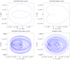Fig. 1. Dynamical substitutes of ℒ3 in the Sun–Earth–Venus, Sun–Earth–Jupiter, Sun–Earth–Venus–Jupiter and complete systems obtained by integration. For the Sun–Earth–Venus–Jupiter and in the complete system the time-span is about 50 years. For all these cases we assume that ${\overline{\varphi }}_j=0$ for j ≠ 3. The red point indicates the position of L3.

In this context, it is natural to construct canonical transformations using the Lie method: given a generating function χ(Λ, Φ, λ, φ, θ), the Hamiltonian flow generated by χ at time t = 1 is a canonical transformation:

$$\begin{array}{c}\hfill {\varphi }_{\chi }^1:(\stackrel{\sim }{\mathrm{\Lambda }},\stackrel{\sim }{\mathrm{\Phi }},\stackrel{\sim }{\mathrm{\Theta }},\stackrel{\sim }{\lambda },\stackrel{\sim }{\phi },\stackrel{\sim }{\theta })\mapsto (\mathrm{\Lambda },\mathrm{\Phi },\mathrm{\Theta },\lambda ,\phi ,\theta ),\end{array}$$

which can be represented by the Lie series:

$$\begin{array}{c}\hfill \begin{array}{cc}& \mathrm{\Lambda }=\stackrel{\sim }{\mathrm{\Lambda }}+\{\stackrel{\sim }{\mathrm{\Lambda }},\chi \}+\frac{1}{2}\{\{\stackrel{\sim }{\mathrm{\Lambda }},\chi \},\chi \}+\dots \hfill \\ \hfill & \mathrm{\Phi }=\stackrel{\sim }{\mathrm{\Phi }}+\{\stackrel{\sim }{\mathrm{\Phi }},\chi \}+\frac{1}{2}\{\{\stackrel{\sim }{\mathrm{\Phi }},\chi \},\chi \}+\dots \hfill \\ \hfill & \mathrm{\Theta }=\stackrel{\sim }{\mathrm{\Theta }}+\{\stackrel{\sim }{\mathrm{\Theta }},\chi \}+\frac{1}{2}\{\{\stackrel{\sim }{\mathrm{\Theta }},\chi \},\chi \}+\dots \hfill \\ \hfill & \lambda =\stackrel{\sim }{\lambda }+\{\stackrel{\sim }{\lambda },\chi \}+\frac{1}{2}\{\{\stackrel{\sim }{\lambda },\chi \},\chi \}+\dots \hfill \\ \hfill & \phi =\stackrel{\sim }{\phi }+\{\stackrel{\sim }{\phi },\chi \}+\frac{1}{2}\{\{\stackrel{\sim }{\phi },\chi \},\chi \}+\dots \hfill \\ \hfill & {\theta }_j={\stackrel{\sim }{\theta }}_j,\hfill \end{array}\end{array}$$(9)

where { , } denote the Poisson brackets, and conjugates the Hamiltonian 𝒲 to

$$\begin{array}{cc}\hfill \stackrel{\sim }{\mathcal{W}}& =\mathcal{W}°{\varphi }_{\chi }^1(\stackrel{\sim }{\mathrm{\Lambda }},\stackrel{\sim }{\mathrm{\Phi }},\stackrel{\sim }{\mathrm{\Theta }},\stackrel{\sim }{\lambda },\stackrel{\sim }{\phi },\stackrel{\sim }{\theta })\hfill \\ \hfill & =\mathcal{W}+\{\mathcal{W},\chi \}+\frac{1}{2}\{\{\mathcal{W},\chi \},\chi \}+\dots \hfill \end{array}$$

The normal form 𝒲 does not depend on the planetary anomalies at first order in the planetary masses if we define the generating function by

$$\begin{array}{c}\hfill \chi :={\displaystyle \sum _{j\ne 3}}{\epsilon }_j{\chi }_j,{\chi }_j={\displaystyle \sum _{i_2,i_3\in Z}}{\widehat{\chi }}_{i_2,i_3}^j(\stackrel{\sim }{\mathrm{\Lambda }},\stackrel{\sim }{\mathrm{\Phi }})sin((i_2+i_3)\stackrel{\sim }{\lambda }+i_2\stackrel{\sim }{\phi }+i_3{\stackrel{\sim }{\theta }}_j),\end{array}$$(10)

with

$$\begin{array}{c}\hfill {\widehat{\chi }}_{i_2,i_3}^j:={\delta }_{i_3}\frac{{\widehat{\mathcal{W}}}_{i_2,i_3}^j}{(i_2+i_3){\omega }_{\lambda }+i_2{\omega }_{\phi }+i_3{\omega }_{{\theta }_j}},\end{array}$$

where δ₀ = 0, δ_i = 1 if i ≠ 0, and ${\omega }_{\lambda }=\frac{\partial {\mathcal{W}}_0}{\partial \stackrel{\sim }{L}}$, ${\omega }_{\phi }=\frac{\partial {\mathcal{W}}_0}{\partial \stackrel{\sim }{\mathrm{\Phi }}}$, and ${\omega }_{{\theta }_j}={\overline{n}}_j$. Precisely, the normal form corresponding to this generating function can be represented by:

$$\mathcal{W}°{\varphi }_{\chi }^1(\stackrel{\sim }{\mathrm{\Lambda }},\stackrel{\sim }{\mathrm{\Phi }},\stackrel{\sim }{\mathrm{\Theta }},\stackrel{\sim }{\lambda },\stackrel{\sim }{\phi },\stackrel{\sim }{\theta })=\overline{\mathcal{W}}(\stackrel{\sim }{\mathrm{\Lambda }},\stackrel{\sim }{\mathrm{\Phi }},\stackrel{\sim }{\lambda },\stackrel{\sim }{\phi })+{\displaystyle \sum _{j\ne 3}}{\overline{n}}_j{\stackrel{\sim }{\mathrm{\Theta }}}_j+\mathcal{O}\left({\epsilon }^2\right),$$

with ε² = ∑_j ≠ 3ε₃ε_j and

$$\begin{array}{cc}\hfill \overline{\mathcal{W}}& ={\mathcal{W}}_0(\stackrel{\sim }{\mathrm{\Lambda }},\stackrel{\sim }{\mathrm{\Phi }})+{\epsilon }_3{\mathcal{W}}_3(\stackrel{\sim }{\mathrm{\Lambda }},\stackrel{\sim }{\mathrm{\Phi }},\stackrel{\sim }{\lambda },\stackrel{\sim }{\phi })\hfill \\ \hfill & +{\displaystyle \sum _{j\ne 3}}{\displaystyle \sum _{i_2\in Z}}{\epsilon }_j{\widehat{\mathcal{W}}}_{i_2,0}^j(\stackrel{\sim }{\mathrm{\Lambda }},\stackrel{\sim }{\mathrm{\Phi }})cos\left(i_2(\stackrel{\sim }{\lambda }+\stackrel{\sim }{\phi })\right).\hfill \end{array}$$

By introducing the averaged Cartesian coordinates (${\stackrel{\sim }{P}}_X,{\stackrel{\sim }{P}}_Y,$ $\stackrel{\sim }{X},\stackrel{\sim }{Y}$) from the averaged modified Delaunay variables (see Eq. (3)):

$$\begin{array}{c}\hfill ({\stackrel{\sim }{P}}_X,{\stackrel{\sim }{P}}_Y,\stackrel{\sim }{X},\stackrel{\sim }{Y})=\mathcal{D}(\stackrel{\sim }{\mathrm{\Lambda }},\stackrel{\sim }{\mathrm{\Phi }},\stackrel{\sim }{\lambda },\stackrel{\sim }{\phi },),\end{array}$$

we have $\overline{H}=\overline{\mathcal{W}}°{\mathcal{D}}^{-1}$ and

$$\begin{array}{cc}& {\mathcal{W}}_0°{\mathcal{D}}^{-1}=\frac{{\stackrel{\sim }{P}}_X^2+{\stackrel{\sim }{P}}_Y^2}{2}-\frac{\mu }{\sqrt{{\stackrel{\sim }{X}}^2+{\stackrel{\sim }{Y}}^2}}-n_3(\stackrel{\sim }{X}{\stackrel{\sim }{P}}_Y-\stackrel{\sim }{Y}{\stackrel{\sim }{P}}_X),\hfill \\ \hfill & {\epsilon }_3{\mathcal{W}}_3°{\mathcal{D}}^{-1}={\epsilon }_3(\frac{\stackrel{\sim }{X}}{d_3^2}-\frac{1}{\sqrt{{(\stackrel{\sim }{X}-d_3)}^2+{\stackrel{\sim }{Y}}^2}})·\hfill \end{array}$$

Finally, by representing $(\stackrel{\sim }{X},\stackrel{\sim }{Y})=\sqrt{{\stackrel{\sim }{X}}^2+{\stackrel{\sim }{Y}}^2}(cosf,sinf)$ and introducing ${\beta }_j=(f-{\stackrel{\sim }{\theta }}_j)/2$, we have

$$\begin{array}{c}\hfill \begin{array}{cc}& \sum _{i_2\in Z}{\epsilon }_j{\widehat{\mathcal{W}}}_{i_2,0}^{j}cos\left(i_2(\stackrel{\sim }{\lambda }+\stackrel{\sim }{\phi })\right)°{\mathcal{D}}^{-1}=\frac{{\epsilon }_j}{2\pi }{\int }_0^{2\pi }[\frac{\stackrel{\sim }{X}cos{\stackrel{\sim }{\theta }}_j}{d_j^2}\hfill \\ \hfill & +\frac{\stackrel{\sim }{Y}sin{\stackrel{\sim }{\theta }}_j}{d_j^2}-\frac{1}{\sqrt{{(\stackrel{\sim }{X}-d_{j}cos{\stackrel{\sim }{\theta }}_j)}^2+{(\stackrel{\sim }{Y}-d_{j}sin{\stackrel{\sim }{\theta }}_j)}^2}}]\text{d}{\stackrel{\sim }{\theta }}_j\hfill \\ \hfill & =-\frac{2{\epsilon }_j}{\pi }{\int }_0^{\frac{\pi }{2}}\frac{\text{d}{\beta }_j}{\sqrt{{(\sqrt{{\stackrel{\sim }{X}}^2+{\stackrel{\sim }{Y}}^2}-d_j)}^2+4d_j\sqrt{{\stackrel{\sim }{X}}^2+{\stackrel{\sim }{Y}}^2}{sin}^2{\beta }_j}}\hfill \\ \hfill & =-\frac{2{\epsilon }_j}{\pi \mid \sqrt{{\stackrel{\sim }{X}}^2+{\stackrel{\sim }{Y}}^2}-d_j\mid }\mathcal{K}(-\frac{4d_j\sqrt{{\stackrel{\sim }{X}}^2+{\stackrel{\sim }{Y}}^2}}{{(\sqrt{{\stackrel{\sim }{X}}^2+{\stackrel{\sim }{Y}}^2}-d_j)}^2}).\hfill \end{array}\end{array}$$

2.3. Dynamics of the averaged Hamiltonian (2) close to ℒ₃

The Hamiltonian (2) admits an equilibrium point on the axis $\stackrel{\sim }{Y}=0$ close to the Lagrangian point L₃ of the CR3BP, which we denote by ℒ₃. More precisely, Hamiltonian (2) is a small perturbation of the Hamiltonian of the Sun–Earth CR3BP depending on ${\stackrel{\sim }{Y}}^2$. Therefore, on the one hand the equation:

$$\begin{array}{c}\hfill \frac{\partial \overline{H}}{\partial \stackrel{\sim }{Y}}({\stackrel{\sim }{P}}_X,{\stackrel{\sim }{P}}_Y,\stackrel{\sim }{X},\stackrel{\sim }{Y})=0\end{array}$$

is satisfied by any $({\stackrel{\sim }{P}}_X,{\stackrel{\sim }{P}}_Y,\stackrel{\sim }{X},\stackrel{\sim }{Y})$ with $\stackrel{\sim }{Y}=0,{\stackrel{\sim }{P}}_X=0$; on the other hand the equation

$$\begin{array}{c}\hfill \frac{\partial \overline{H}}{\partial \stackrel{\sim }{X}}(0,{\stackrel{\sim }{P}}_Y,\stackrel{\sim }{X},0)=0\end{array}$$

has a solution $X_{{\mathcal{L}}_3},{\stackrel{\sim }{P}}_Y=n_3{X}_{{\mathcal{L}}_3}$ with X_ℒ3 close to X_L3. By including in the model all the planets from Mercury to Neptune we find X_ℒ3 − X_ℒ3 ∼ −2.58 10⁻⁷ AU ∼ −39 km. More precisely, by computing the individual contribution of each planet to the displacement of ℒ₃ from L₃ (see Table 1, where the individual contribution of a planet is computed by setting to zero the masses of all other planets, except for the Earth) we find that Venus and Jupiter each move the position of this equilibrium by about 218 and 176 km, respectively, in opposite directions; in the model where both the planets are included, their effects almost perfectly compensate for one another, leaving a displacement of about 40 km only. Table 1 shows that the individual contributions of the planets to the eigenvalues of the linearization matrix at ℒ₃ are very small, and do not affect the nature of the equilibrium, which remains partially hyperbolic. As a consequence, around ℒ₃ we find a family of periodic orbits, namely the Lyapunov orbits of ℒ₃.

2.4. The dynamical substitute: mapping ℒ₃ back to the original Cartesian variables

The equilibrium point ℒ₃ is finally mapped back to the original Cartesian variables P_X, P_Y, X, Y using the canonical transformation defined by the Hamiltonian flow at “time 1” of the generating function $\chi (\stackrel{\sim }{\mathrm{\Lambda }},\stackrel{\sim }{\mathrm{\Phi }},\stackrel{\sim }{\lambda },\stackrel{\sim }{\phi },\stackrel{\sim }{\theta })$ introduced in Eq. (10). Since the orbital elements of ℒ₃ are characterized by a very small eccentricity (about 10⁻⁶), it is mandatory to represent the generating function χ using the Poincaré variables $\stackrel{\sim }{\mathrm{\Lambda }}$, $\stackrel{\sim }{p}$, $\stackrel{\sim }{\lambda }$, $\stackrel{\sim }{q}$, where $\stackrel{\sim }{p},\stackrel{\sim }{q}$ are related to $\stackrel{\sim }{\mathrm{\Phi }},\stackrel{\sim }{\phi }$ by

$$\begin{array}{c}\hfill \stackrel{\sim }{p}=\sqrt{2\stackrel{\sim }{\mathrm{\Phi }}}cos\stackrel{\sim }{\phi },\stackrel{\sim }{q}=\sqrt{2\stackrel{\sim }{\mathrm{\Phi }}}sin\stackrel{\sim }{\phi }.\end{array}$$

Moreover, since for the times required by astrodynamics we are allowed to neglect in the transformation the terms proportional to the product of two planetary masses, we approximate the Lie series generated by χ with

$$\begin{array}{c}\hfill \begin{array}{cc}& \mathrm{\Lambda }=\stackrel{\sim }{\mathrm{\Lambda }}+\{\stackrel{\sim }{\mathrm{\Lambda }},\chi \},p=\stackrel{\sim }{p}+\{\stackrel{\sim }{p},\chi \}\hfill \\ \hfill & \lambda =\stackrel{\sim }{\lambda }+\{\stackrel{\sim }{\lambda },\chi \},q=\stackrel{\sim }{q}+\{\stackrel{\sim }{q},\chi \}.\hfill \end{array}\end{array}$$(11)

Taking advantage of the small value of the eccentricity of ℒ₃, the numerical computation of the right-hand sides of Eq. (11) can be done by neglecting the terms depending on $\stackrel{\sim }{p},\stackrel{\sim }{q}$ at orders equal to or higher than four and for $\stackrel{\sim }{\theta }=({\overline{n}}_{1}t+{\overline{\varphi }}_1,\dots ,{\overline{n}}_{8}t+{\overline{\varphi }}_8)$. Finally, we transform back to the Cartesian variables and we obtain the dynamical substitute of ℒ₃ as a quasi-periodic function of time:

$$\begin{array}{cc}& (P_{X,{\mathcal{L}}_3}(t),P_{Y,{\mathcal{L}}_3}(t),X_{{\mathcal{L}}_3}(t),Y_{{\mathcal{L}}_3}(t))\hfill \\ \hfill & :=(P_X\left(\stackrel{\sim }{\theta }\right),P_Y\left(\stackrel{\sim }{\theta }\right),X\left(\stackrel{\sim }{\theta }\right),Y\left(\stackrel{\sim }{\theta }\right)).\hfill \end{array}$$(12)

In the simpler bi-circular four-body problems, Sun–Earth–(j-th planet), the dynamical substitute $(P_{X,{\mathcal{L}}_3}(t),P_{Y,{\mathcal{L}}_3}(t),X_{{\mathcal{L}}_3}(t),Y_{{\mathcal{L}}_3}(t))$ is a periodic function of time with frequency ${\overline{n}}_j$. In order to verify that there is a real orbit for the restricted problem that remains close to the dynamical substitute (X_ℒ3(t),Y_ℒ3(t)) for times that are of interest for astrodynamics, we numerically integrate the equations of motion of the restricted problem with initial conditions $(P_X(0),P_Y(0),X(0),Y(0))=(P_{X,{\mathcal{L}}_3}(0),P_{Y,{\mathcal{L}}_3}(0),X_{{\mathcal{L}}_3}(0),Y_{{\mathcal{L}}_3}(0))$. In Fig. 1 we present the dynamical substitutes of ℒ₃ computed by integrating the initial datum for four cases: the Sun–Earth–Venus, Sun–Earth–Jupiter, Sun–Earth–Venus–Jupiter, and the complete system (namely the system containing all eight planets) with ${\overline{\varphi }}_j=0$ for all j ≠ 3. In Table 1 we also present the libration amplitudes for each restricted Sun–Earth–(j-th planet) problem. We find that in the MCR8BP, the orbit is a quasi-periodic oscillation around L₃ with amplitude d ∼ 10⁻⁴ AU. Each orbit in a neighborhood of ℒ₃ can be mapped back to the original Cartesian variables using the canonical transformations (11) and 𝒟; for example, the periodic Lyapunov orbits will be mapped back to quasi-periodic orbits of amplitudes larger than d. Therefore, in the MCR8BP we have a family of quasi-periodic oscillations around L₃ of amplitudes α >  d.

3. The fast Lyapunov indicator method and the computation of the librations in a realistic model of the Solar System

As the restricted multicircular model represents just a simplified model of our Solar System, we must investigate whether or not orbits close to L₃ still exist when the trajectories of the planets are realistic. Furthermore, as the effects of Mercury on both the dynamical substitute and in the change of the other planets ephemerides are negligible for the short time intervals that we are taking into account, we consider a model of the Solar System that includes the planets from Venus to Neptune. We use r = (x, y, z) and v = (v_x, v_y, v_z) to denote the position and velocity vectors of the spacecraft, and r_j = (x_j, y_j, z_j) and v_j = (v_x, j, v_y, j, v_z, j) the position and velocity vector of the j-th planet in the Heliocentric reference frame. To identify a configuration generalizing the Lagrangian point L₃ of the CR3BP in this more realistic system, we first introduce a Heliocentric rotating-pulsating reference frame OXYZ, whose Cartesian axes are parallel, at any time t, to the unit vectors

$$\begin{array}{c}\hfill {\mathit{e}}_r=\frac{{\mathit{r}}_3}{\Vert {\mathit{r}}_3\Vert },{\mathit{e}}_n=\frac{{\mathit{v}}_3\times {\mathit{r}}_3}{\Vert {\mathit{v}}_3\times {\mathit{r}}_3\Vert },{\mathit{e}}_t=\frac{{\mathit{r}}_3\times {\mathit{e}}_n}{\Vert {\mathit{r}}_3\times {\mathit{e}}_n\Vert }·\end{array}$$

In a such reference frame, the Earth state vector is (1, 0, 0, 0, 0, 0) at any time t. We apply the FLI method in order to find orbits staying close to L₃ in the realistic model for centuries; this method provides initial conditions of trajectories remaining in a given neighborhood ℬ of a libration orbit found in an approximated model. For the definition of ℬ we have to consider both the amplitude of the libration orbit and the differences between the realistic model and the CR3BP due to Earth’s elliptic orbit. Hence, for the application of the FLI method we first compute a planar Lyapunov orbit of the CR3BP with amplitude α and then we use this orbit to find librations in the ER3BP remaining close to it. We denote these librations by ℓ(α) and the details of their computation are explained in Sect. 3.2. By assuming that the planetary perturbations introduce additional oscillations of amplitude d comparable to those found in the MCR8BP, we finally look for hyperbolic orbits of the realistic model which remain in a neighborhood of radius 2d of the reference orbit ℓ(α) for centuries (Sect. 3.3). We compute both ℓ(α) of the ER3BP for different orders of the amplitude and the libration orbits in the realistic model of the Solar System using the recent version of the modified FLI method.

3.1. The FLI method

The FLI method was originally introduced by Froeschlé et al. (1997a,b) to numerically distinguish between regular and chaotic orbits. In recent years, the method has been modified in order to compute hyperbolic orbits of dynamical systems and their asymptotic solutions: Guzzo & Lega (2014, 2018), and Lega & Guzzo (2016) provide a detailed theoretical justification of the method, with a focus on the computation of transit orbits of the Sun-Jupiter system in the circular restricted three-body problem; in Guzzo & Lega (2015, 2017) the method has been adapted to compute the collision manifold of the comet 67P/Churyumov-Gerasimenko in a model of the Solar System that is compatible with the JPL ephemerides. In this paper, for the first time, the modified version of the FLI method is used to investigate the dynamics originating at a Lagrangian equilibrium point in a realistic model of the Solar System. Moreover, since we are considering the point L₃ of the Sun–Earth system, the CR3BP provides only a very crude approximation. The extension from the CR3BP problem to the realistic one required a new strategy based on the preliminary study of intermediate models to include the planetary perturbations and the eccentricity of Earth’s orbit. In this way we first find the orbits ℓ(α) of the Sun–Earth ER3BP, and then the libration orbits of the realistic model of the Solar System. In particular, this usage of the chaos indicator provides an innovative and novel application of dynamical systems theory to astrodynamics, where the short-period perturbations represent a relevant part of the model.

The modified FLI is introduced as follows. We first consider the spacecraft equations of motion written as a system of first-order differential equations:

$$\begin{array}{c}\hfill \dot{\mathit{\xi }}=F(\mathit{\xi },t),\end{array}$$(13)

where ξ denotes the state vector of the spacecraft in a given reference frame. For simplicity, we choose as epoch t = 0 the time of an Earth passage to the perihelion. The variational equations of (13) are

$$\begin{array}{c}\hfill \dot{\mathbf{\Xi }}=[\frac{\partial F}{\partial \mathit{\xi }}(\mathit{\xi },t)]\mathbf{\Xi },\mathbf{\Xi }\in {\mathbb{R}}^6,\end{array}$$(14)

where $\frac{\partial F}{\partial \mathit{\xi }}$ denotes the Jacobian matrix of F. If we aim to find the hyperbolic orbits that remain in a neighborhood ℬ of a given target orbit γ for as long as possible, we introduce the window function w(R) and the modified FLI defined as

$$\begin{array}{c}\hfill w(\mathit{R})=\{\begin{array}{c}1\text{if}\mathit{R}\in \mathcal{B}\hfill \\ 0\text{otherwise}\hfill \end{array}\end{array}$$

$$\begin{array}{c}\hfill \text{mFLI}({\mathit{\xi }}_0,{\mathbf{\Xi }}_0;T):={\displaystyle \underset{t\in [0,T]}{max}}{{\displaystyle \int }}_0^{t}max(0,w(\mathit{R}(s))\frac{\mathbf{\Xi }(s)·\dot{\mathbf{\Xi }}(s)}{{\Vert \mathbf{\Xi }(s)\Vert }^2})\text{d}s,\end{array}$$(15)

respectively, where R(s) is the position vector of the spacecraft in the rotating-pulsating reference frame computed by integrating the differential equations (13) with initial conditions ξ₀, and Ξ(s) is the solution of the variational equations (14) with Ξ₀ as initial tangent vector. When the target orbit γ is partially hyperbolic and ℬ is suitably small, the only possibility for an orbit to increase the modified FLI to the highest possible values is to remain very close to the target over the whole time interval [0, T]. Here, we have the two possible cases: (i) a large measure set ℬ_I ⊂ ℬ of initial conditions corresponds to solutions that exit from ℬ in short times T₀ and whose mFLI does not increase for T >  T₀; (ii) a small measure set ℬ_II ⊂ ℬ corresponds to solutions which do not exit from ℬ, remain close to a partially hyperbolic orbit of ℬ, and whose mFLI increases linearly with time T (Guzzo & Lega 2014). Orbits that come back to (or enter) the set ℬ, but do not stay close to the target over the time interval of interest [0, T] necessarily enter the set ℬ_I and exit from ℬ in a short time T₀. Therefore, the modified FLI sharply identifies the orbits (II) when it is computed on grids of initial conditions that are transverse to ℬ_II. The key factor for the success of the method is the suitable choice of the set ℬ and of the grid of initial conditions, which is suggested by the application of perturbation theories and approximated models.

3.2. Computation of libration orbits in the ER3BP

The Sun–Earth ER3BP deals with the study of the spacecraft dynamics gravitationally attracted by the Sun and the Earth while the latter performs an elliptic motion around the barycenter of the Sun–Earth system; in order to compare the ER3BP with the CR3BP, the equations of motion of the ER3BP are typically described in the rotating-pulsating reference frame (Szebehely 1967). In order to find the orbits ℓ(α) of the ER3BP, we use the modified FLI (15) using a planar Lyapunov orbit of the CR3BP of libration amplitude α as target orbit γ. The set ℬ is a neighborhood of γ with amplitude $\stackrel{\sim }{d}$; if (X₀, 0, 0, 0, V_Y, 0, 0) is a point of the target Lyapunov orbit, we choose the grid of initial data as the set (X₀, 0, 0, 0, V_Y, 0), where V_Y is evenly spaced over some interval. The extrema of this latter interval are chosen such that it contains a strict maximum of the modified FLI. We then restrict this interval around the maximum and repeat the computation of the FLI for the new grid and for a longer integration time. The procedure is iterated until we achieve a sufficiently long integration time. In Fig. 2 we show the results of the method for a time-span of 1000 years and for values of α equal to 3 × 10⁻², 10⁻³, and 10⁻⁴ AU, correspondingly to $\stackrel{\sim }{d}$ equal to 10⁻³, 7 × 10⁻⁵, and 10⁻⁵ AU. We note that such orbits are slowly drifting along the Y axis (at a speed of about 2 × 10⁻⁶, 5 × 10⁻⁸ and 4.5 × 10⁻⁹ AU yr⁻¹ for ℓ(3 × 10⁻² AU), ℓ(10⁻³ AU), and ℓ(10⁻⁴ AU), respectively): these drifts can be reduced by further refining the interval of the initial data.

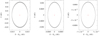Fig. 2. Representation of ℓ(α) orbits (gray lines) of the ER3BP in the rotating-pulsating reference frame with α = 3 × 10−2, 10−3, 10−4 AU for 1000 years. The values of $\stackrel{\sim }{d}$ in the three different cases are 10−3, 7 × 10−5, and 10−5 AU. The representation of ℓ(α) in the time-span of 1 year (black curves) emphasizes the small drifts of the librations along the Y axis. The red point indicates the position of L3.

3.3. Computation of the libration orbits in the realistic model of the Solar System

In order to study the spacecraft dynamics in a model whose ephemerides are comparable with those provided by the JPL computation service, we consider the spacecraft equations of motion in the barycentric reference frame in a model composed of the Sun and seven planets whose initial conditions are provided by JPL (for the Earth we consider the Earth–Moon barycenter). To illustrate how to find libration orbits in such a realistic model, we apply the FLI method and we consider ℓ(3 × 10⁻² AU) and ℓ(10⁻³ AU) as target orbits and take ℬ as a neighborhood of ℓ(3 × 10⁻² AU) and ℓ(10⁻³ AU) of amplitude $\stackrel{\sim }{d}$ equal to 10⁻³ and 2 × 10⁻⁴ AU, respectively. The computation of the modified FLI is stopped once we have restricted the set of initial data such that the interval along the V_Y is smaller than 5 × 10⁻⁹ AU day⁻¹ and once we achieve an integration time of centuries (in the cases of the librations with amplitudes of 3 × 10⁻² and 10⁻³ AU the time-spans for the modified FLI computation are 1000 and 400 years respectively). When we conclude this iterative method, we obtain the modified FLI profile, in which the maximum is sharply identified by the initial datum $(X_0,0,0,0,V_Y^{\ast },0)$. For example, the modified FLI profile for the research of the libration with amplitude 3 × 10⁻² AU is represented in Fig. 3. The trajectory associated to the initial datum with the maximum mFLI value (blue point in Fig. 3) represents the orbit that remains the closest to the target one. Moreover, this trajectory (see the first two panels in Fig. 4) is librating around L₃ with an amplitude of 3 × 10⁻² AU. To appreciate the precision of the method, we also considered the orbits associated to another two initial data with values of the modified FLI that are different from the maximum (the magenta and brown points in Fig. 3). Such orbits, shown in Fig. 5, are not librations around L₃, even if the variation of the initial velocity $V_Y-V_Y^{\ast }$ is very small (about 3 × 10⁻¹² and −3 × 10⁻¹¹ AU day⁻¹, respectively). Now, we focus our attention on the orbits associated to the maximum value of mFLI for both the case of ℓ(3 × 10⁻² AU) and ℓ(10⁻³ AU) as target orbits. These trajectories are shown in Fig. 4 in the time-spans of 650 and 200 years respectively. In the same figure we also show the representations of such trajectories restricted to a time-span of 20 years (black curves) which highlight the drift along the Y axis (about 4 × 10⁻⁶ AU yr⁻¹) caused by the planetary perturbations. The relative drift is greater for the libration with amplitude 10⁻³ AU and is smaller for the orbit with greater amplitude. Hence, the orbit with the greater amplitude remains closer to its target orbit. Moreover, the value of $\stackrel{\sim }{d}$ for the orbit with smaller amplitude is close to the amplitude of the oscillation introduced by the planetary perturbations (last panel in Fig. 1): this implies that values of $\stackrel{\sim }{d}<2d$ are too small and for such a choice of $\stackrel{\sim }{d,}$ the FLI method does not converge to a libration orbit around L₃. Therefore, to find oscillations around L₃ with amplitudes smaller than 2d it is necessary to apply the FLI method by using a sphere in (X, Y, Z) centered at L₃ with radius $\stackrel{\sim }{d}\le 2d$ as ℬ. We note also that the application of the modified FLI method with a one-dimensional grid of initial data is not sufficient for the research of librations because of the degrees of freedom of the problem: we have to use a two-dimensional grid of initial data (X, 0, 0, 0, V_Y, 0) centered at L₃. Therefore, we applied this method with $\stackrel{\sim }{d}={10}^{-3}$ and $\stackrel{\sim }{d}=2\times {10}^{-4}$ AU and found (see e.g., Fig. 6) that the bigger values of the mFLI lie on a line not parallel to the X and V_Y axis. This complicates the procedure of refining the initial data, which is summarized in the caption of the figure. Finally, Fig. 7 shows the librations obtained using the two-dimensional grid with $\stackrel{\sim }{d}={10}^{-3}$ and $\stackrel{\sim }{d}=2\times {10}^{-4}$ AU: the time-spans of these two orbits are 700 and 250 years respectively. Hence, the FLI method allows us to find libration orbits of the realistic models with amplitudes bigger than d (up to 0.03 AU) for time-spans of centuries.

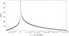Fig. 3. Profile of the modified FLI for the time-span of 1000 years in the case of the research of the libration with amplitude 3 × 10−2 AU in the realistic model. The blue point denotes the location of $V_Y^{\ast }$, namely the velocity component along Y characterized by the maximum mFLI value, and the trajectory associated to the initial condition $(X_0,0,0,0,V_Y^{\ast },0)$ is shown in the first two panels of Fig. 4. We also show the locations of another two initial conditions (the magenta and brown point) with a different value of the chaos indicator whose trajectories are plotted in Fig. 5.

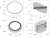Fig. 4. Representation of the librations around L3 in the realistic model obtained by changing the target orbit ℓ(α) and $\stackrel{\sim }{d}$. The first two figures represent the librations found by using ℓ(3 × 10−2 AU) and ℓ(10−3 AU), respectively. The black lines represent the restriction of the trajectories to 20 years. The red point indicates the position of L3 in the rotating-pulsating reference frame.

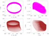Fig. 5. Trajectories associated to the magenta and brown point in Fig. 3. The time-span for both orbits is 650 years. The plots highlight the precision of the modified FLI method. Small displacements of the initial conditions corresponding to the maximum mFLI value lead to large differences in the orbits: in this scenario, the variation of the initial velocity $V_Y-V_Y^{\ast }$ is about 3 × 10−12 and −3 × 10−11 AU day−1 for the magenta and brown trajectories. Both orbits are escaping from L3.

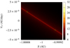Fig. 6. Representation of the modified FLI map associated to the bidimensional grid of initial data in the case in which L3 is the reference point and $\stackrel{\sim }{d}={10}^{-3}$; the colors indicate the values of the chaos indicator computed in the time-span of 1000 years. We note that the maximum values of mFLI are not in a line parallel to the X or VY axis. For this reason, if we want to have a good refinement of the two-dimensional grid, we need to isolate two points P0 = (X0, VY, 0), P1 = (X1, VY, 1) (green points) of the two-dimensional grid characterized by a high value of the modified FLI and then take points X and VY such that X = X0 + δ(X1 − X0)+ϵ(VY, 1 − VY, 0), VY = VY, 0 + δ(VY, 1 − VY, 0)−ϵ(X1 − X0) with δ ∈ [0, 1] and ϵ ∈ [ − Δϵ, Δϵ]: we used Δϵ equal to 2 × 10−5 for the refinement of the grid shown in this figure.

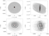Fig. 7. Representation of the librations around L3 in the realistic model obtained assuming a neighborhood of L3 with amplitude $\stackrel{\sim }{d}$ equal to 10−3 and 2 × 10−4 AU, respectively. The time-spans of the two orbits are 700 and 250 years respectively. The black lines represent the restriction of the trajectories to 20 years. The red point indicates the position of L3 in the rotating-pulsating reference frame.

4. Conclusions

Since close to the Sun–Earth Lagrangian point L₃ the planetary perturbations (mainly from Jupiter and Venus) are stronger than Earth’s attraction, it is not evident that the dynamics close to L₃ defined within the circular restricted three-body problem can be continued to a realistic model of the Solar System. We analyze in particular the effects of the planetary perturbations and of the eccentricity of the Earth. The planetary perturbations provide oscillations of about 15 000 km, while the effect of the eccentricity of the Earth, apart from a small oscillation, is absorbed by considering a rotating-pulsating frame. Using a combination of the Hamiltonian averaging method with the FLI method we find orbits that remain close to L₃ for at least 200 years in a model of the Solar System whose dynamics are compatible with JPL digital ephemerides, with libration amplitudes ranging from 2.5 × 10⁻⁴ to 3 × 10⁻² AU.

Acknowledgments

We thank the anonymous referee for useful remarks and suggestions. M.G. acknowledges the project MIUR-PRIN 20178CJA2B “New frontiers of Celestial Mechanics: theory and applications”.

References

All Tables

All Figures

	Fig. 1. Dynamical substitutes of ℒ3 in the Sun–Earth–Venus, Sun–Earth–Jupiter, Sun–Earth–Venus–Jupiter and complete systems obtained by integration. For the Sun–Earth–Venus–Jupiter and in the complete system the time-span is about 50 years. For all these cases we assume that ${\overline{\varphi }}_j=0$ for j ≠ 3. The red point indicates the position of L3.
In the text

Fig. 2. Representation of ℓ(α) orbits (gray lines) of the ER3BP in the rotating-pulsating reference frame with α = 3 × 10−2, 10−3, 10−4 AU for 1000 years. The values of $\stackrel{\sim }{d}$ in the three different cases are 10−3, 7 × 10−5, and 10−5 AU. The representation of ℓ(α) in the time-span of 1 year (black curves) emphasizes the small drifts of the librations along the Y axis. The red point indicates the position of L3.

In the text

Fig. 3. Profile of the modified FLI for the time-span of 1000 years in the case of the research of the libration with amplitude 3 × 10−2 AU in the realistic model. The blue point denotes the location of $V_Y^{\ast }$, namely the velocity component along Y characterized by the maximum mFLI value, and the trajectory associated to the initial condition $(X_0,0,0,0,V_Y^{\ast },0)$ is shown in the first two panels of Fig. 4. We also show the locations of another two initial conditions (the magenta and brown point) with a different value of the chaos indicator whose trajectories are plotted in Fig. 5.

In the text

Fig. 4. Representation of the librations around L3 in the realistic model obtained by changing the target orbit ℓ(α) and $\stackrel{\sim }{d}$. The first two figures represent the librations found by using ℓ(3 × 10−2 AU) and ℓ(10−3 AU), respectively. The black lines represent the restriction of the trajectories to 20 years. The red point indicates the position of L3 in the rotating-pulsating reference frame.

In the text

Fig. 5. Trajectories associated to the magenta and brown point in Fig. 3. The time-span for both orbits is 650 years. The plots highlight the precision of the modified FLI method. Small displacements of the initial conditions corresponding to the maximum mFLI value lead to large differences in the orbits: in this scenario, the variation of the initial velocity $V_Y-V_Y^{\ast }$ is about 3 × 10−12 and −3 × 10−11 AU day−1 for the magenta and brown trajectories. Both orbits are escaping from L3.

In the text

Fig. 6. Representation of the modified FLI map associated to the bidimensional grid of initial data in the case in which L3 is the reference point and $\stackrel{\sim }{d}={10}^{-3}$; the colors indicate the values of the chaos indicator computed in the time-span of 1000 years. We note that the maximum values of mFLI are not in a line parallel to the X or VY axis. For this reason, if we want to have a good refinement of the two-dimensional grid, we need to isolate two points P0 = (X0, VY, 0), P1 = (X1, VY, 1) (green points) of the two-dimensional grid characterized by a high value of the modified FLI and then take points X and VY such that X = X0 + δ(X1 − X0)+ϵ(VY, 1 − VY, 0), VY = VY, 0 + δ(VY, 1 − VY, 0)−ϵ(X1 − X0) with δ ∈ [0, 1] and ϵ ∈ [ − Δϵ, Δϵ]: we used Δϵ equal to 2 × 10−5 for the refinement of the grid shown in this figure.

In the text

Fig. 7. Representation of the librations around L3 in the realistic model obtained assuming a neighborhood of L3 with amplitude $\stackrel{\sim }{d}$ equal to 10−3 and 2 × 10−4 AU, respectively. The time-spans of the two orbits are 700 and 250 years respectively. The black lines represent the restriction of the trajectories to 20 years. The red point indicates the position of L3 in the rotating-pulsating reference frame.

In the text

References

- Barrabés, E., & Ollè, M. 2006, Nonlinearity, 19, 2065 [CrossRef] [Google Scholar]
- Froeschlé, C., Gonczi, R., & Lega, E. 1997a, Planet. Space Sci., 45, 881 [NASA ADS] [CrossRef] [Google Scholar]
- Froeschlé, C., Lega, E., & Gonczi, R. 1997b, Celestial Mech. Dyn. Astron., 67, 41 [NASA ADS] [CrossRef] [MathSciNet] [Google Scholar]
- Gómez, G., & Mondelo, J. 2001, Physica D, 157, 283 [NASA ADS] [CrossRef] [Google Scholar]
- Gómez, G., Llibre, J., Martínez, R., & Simó, C. 2001, in Dynamics and Mission Design Near Libration Points, World Scientific Monograph Series in Mathematics (World Scientific Publishing Co. Inc.), 1 [Google Scholar]
- Gómez, G., Koon, W., Lo, M., et al. 2004, Nonlinearity, 17, 1571 [NASA ADS] [CrossRef] [Google Scholar]
- Guzzo, M., & Lega, E. 2013, MNRAS, 428, 2688 [NASA ADS] [CrossRef] [Google Scholar]
- Guzzo, M., & Lega, E. 2014, Soc. Ind. Appl. Math., 74, 1058 [CrossRef] [Google Scholar]
- Guzzo, M., & Lega, E. 2015, A&A, 579, 1 [NASA ADS] [CrossRef] [EDP Sciences] [Google Scholar]
- Guzzo, M., & Lega, E. 2017, MNRAS, 469, S321 [CrossRef] [Google Scholar]
- Guzzo, M., & Lega, E. 2018, Physica D, 373, 38 [CrossRef] [Google Scholar]
- Hou, X., Tang, J., & Liu, L. 2007, NASA Technical Report: 20080012700 [Google Scholar]
- Jorba, À., & Nicolás, B. 2020, Communications in Nonlinear Science and Numerical Simulation, 89, 105327 [CrossRef] [Google Scholar]
- Koon, W. S., Lo, M. W., Marsden, J. E., & Ross, S. D. 2006, Dynamical Systems, The Three-Body Problem, and Space Mission Design (Pasadena, CA, USA: California Institute of Technology) [Google Scholar]
- Lega, E., & Guzzo, M. 2016, Physica D, 325, 41 [CrossRef] [Google Scholar]
- Lega, E., Guzzo, M., & Froeschlé, C. 2011, MNRAS, 418, 107 [NASA ADS] [CrossRef] [Google Scholar]
- Martin, C., Conway, B. A., & Ibánez, P. 2010, in Space Manifold Dynamics: Novel Spaceways for Science and Exploration, eds. E. Perozzi, & S. Ferraz-Mello (Springer) [Google Scholar]
- Pàez, R., & Efthymiopoulos, C. 2015, Celestial Mech. Dyn. Astron., 121, 139 [CrossRef] [Google Scholar]
- Parker, J., & Anderson, R. L. 2013, Low-Energy Lunar Trajectory Design (Pasadena, CA: Jet Propulsion Laboratory, California Institute of Technology) [Google Scholar]
- Szebehely, V. 1967, Theory of Orbits: The Restricted Problem of Three Bodies (Academic Press) [Google Scholar]
- Tantardini, M., Fantino, E., Ren, Y., et al. 2010, Celestial Mech. Dyn. Astron., 108, 215 [CrossRef] [Google Scholar]
- Terra, M. O., Simó, C., & de Sousa Silva, P. 2014, Proc. IAC, 6, 4535 [Google Scholar]
- van Damme, C. C., Gorgojo, R. C., Gil-Fernandez, J., & Graziano, M. 2010, in Space Manifold Dynamics: Novel Spaceways for Science and Exploration, eds. E. Perozzi, & S. Ferraz-Mello (Springer) [Google Scholar]
All Tables
Displacement Xℒ3 − XL3, differences between the eigenvalues of ℒ3 and L3, and amplitude of the dynamical substitute (DS) along the Y axis for each planet.