| Issue |
A&A
Volume 638, June 2020
|
|
|---|---|---|
| Article Number | A94 | |
| Number of page(s) | 16 | |
| Section | Galactic structure, stellar clusters and populations | |
| DOI | https://doi.org/10.1051/0004-6361/201936557 | |
| Published online | 19 June 2020 | |
Synthetic catalog of black holes in the Milky Way⋆
1
Astronomical Observatory, Warsaw University Ujazdowskie 4, 00-478 Warsaw, Poland
e-mail: This email address is being protected from spambots. You need JavaScript enabled to view it.
2
Center for Theoretical Physics, Polish Academy of Sciences, Al. Lotnikow 32/46, 02-668 Warsaw, Poland
3
Nicolaus Copernicus Astronomical Center, Polish Academy of Sciences, ul. Bartycka 18, 00-716 Warsaw, Poland
4
Harvard-Smithsonian Center for Astrophysics, 60 Garden St, Cambridge, MA 02138, USA
Received:
23
August
2019
Accepted:
7
April
2020
Abstract
Aims. We present an open-access database that includes a synthetic catalog of black holes (BHs) in the Milky Way, divided by the components disk, bulge, and halo.
Methods. To calculate the evolution of single and binary stars, we used the updated population synthesis code StarTrack. We applied a new model of the star formation history and chemical evolution of Galactic disk, bulge, and halo that was synthesized from observational and theoretical data. This model can be easily employed for other studies of population evolution.
Results. We find that at the current Milky Way (disk+bulge+halo) contains about 1.2 × 10⁸ single BHs with an average mass of about 14 M⊙, and 9.3 × 10⁶ BHs in binary systems with an average mass of 19 M⊙. We present basic statistical properties of the BH population in three Galactic components such as the distributions of BH masses, velocities, or the numbers of BH binary systems in different evolutionary configurations.
Conclusions. The metallicity of a stellar population has a significant effect on the final BH mass through the stellar winds. The most massive single BH in our simulation of 113 M⊙ originates from a merger of a BH and a helium star in a low-metallicity stellar environment in the Galactic halo. We constrain that only ∼0.006% of the total Galactic halo mass (including dark matter) can be hidden in the form of stellar origin BHs. These BHs cannot be detected by current observational surveys. We calculated the merger rates for current Galactic double compact objects (DCOs) for two considered common-envelope models: ∼3–81 Myr−1 for BH-BH, ∼1–9 Myr−1 for BH-neutron star (NS), and ∼14–59 Myr−1 for NS-NS systems. We show the evolution of the merger rates of DCOs since the formation of the Milky Way until the current moment with the new star formation model of the Galaxy.
Key words: catalogs / stars: evolution / binaries : close / stars: black holes / Galaxy: stellar content
Data files are available on our website, https://bhc.syntheticuniverse.org/.
© ESO 2020
1. Introduction
The study of the Galactic black hole (BH) population is still a great challenge because BHs themselves do not emit in electromagnetic wavelengths, except for the theoretically predicted Hawking radiation. However, BHs in binary systems can be observed in their interaction with their companion, for example, when a star transfers mass onto the BH1. Binary system with a BH may also be identified by measuring the velocities of the components in wide binary systems (Igoshev & Perets 2019). Recently, after constructing the detector on the Laser Interferometer Gravitational-Wave Observatory (LIGO) and the Michelson interferometer Virgo, double compact object (DCO) systems such as BH-BH, BH-NS, and NS-NS could also be detected through the emission of gravitational waves (Abbott et al. 2016a,b,c, 2017a,b,c; The LIGO Scientific Collaboration & The Virgo Collaboration 2019). Unfortunately, these methods cannot be used in order to detect single BHs, which do not interact with any other massive physical objects. The most promising way to study a single BH population therefore appears to be the gravitational lensing phenomenon (Wyrzykowski et al. 2016a,b). Another possible method that might allow the detection of isolated single and binary BHs is studying the X-ray emission caused by accretion from the dense interstellar medium (ISM; Tsuna et al. 2018). No BH has been detected with this method so far, however.
On the other hand, with access to cosmological population synthesis simulations and theoretical stellar evolution models, the number of Galactic BHs may be predicted in different configurations. Several attempts of such studies have been made in the past. For example, a total number of Milky Way BHs was estimated by Shapiro & Teukolsky (1983), van den Heuvel (1992), Brown & Bethe (1994) and Timmes et al. (1996) at the level of 108 − 109. The population of Galactic BH-BH binaries has been studied using the cosmological simulations by Lamberts et al. (2018). The total number of BH-BH binaries was estimated at ∼1.2 × 10⁶ with the average mass of 28 M⊙ per system. Massive star and DCO binaries were studied using a galactic evolution code (Vanbeveren & Donder 2010; Mennekens & Vanbeveren 2014). Recently, Wiktorowicz et al. (2019) predicted the number of Galactic BHs that formed from binary star systems assuming one Galactic component (disk) and constant star formation rates (SFR) in the Galaxy.
Almost 20 Galactic stellar BHs in binaries are currently observed (Casares 2007; Casares & Jonker 2014)2. Most of them are in X-ray binary systems, where the BH draws matter from its companion through an accretion disk. The average mass of these BHs is about 7.5 M⊙. Discoveries of three BH binary systems have recently been made based on radial velocity measurements (Khokhlov et al. 2018; Thompson et al. 2019; Liu et al. 2019). However, these BH binary systems might not be a representative statistical probe because they are only a small fraction of the whole Galactic BH population. Most Galactic BHs are hard to detect because they do not interact with a companion and might have had a very different evolutionary history. The distributions of BH properties such as masses or velocities might therefore be very different than the distributions shown by the observed binaries.
The Milky Way can be divided into several main components: the bulge, the disk (thin and thick disk), and the halo. These parts are different in their structure, stellar properties (such as chemical composition), formation history, or dynamics. For example, the Galactic disk hosts young stars with high metal content, while the Galactic halo is rather dominated by old and metal-poor stars. In simulations we need to take the metallicity and age distributions of Galactic stellar populations into account based on the recent literature because this strongly influences the course of the evolution of single and binary star systems.
In this article we only consider the evolution of isolated single and binary stars in the Milky Way. In particular, we do not consider dynamical interactions between stars in field populations. Although such interactions are rare, they may lead to some interesting results (e.g., Klencki et al. 2017). We do not consider triple or higher multiplicity stellar systems either. The evolution of such systems may lead to the formation of some exotic configurations and might also enhance BH formation (e.g., Eggleton & Kiseleva-Eggleton 2001; Antonini et al. 2017; Arca-Sedda et al. 2018), but typically, the fraction of stars in higher multiplicity systems is not too large (Raghavan et al. 2010; Duchêne & Kraus 2013). Finally, we do not consider Galactic globular clusters (GCs). As shown by cosmological simulations (Kravtsov & Gnedin 2005) or by measuring the mass-to-light ratio (M/L) (Kruijssen & Mieske 2009), the total mass of Galactic GCs is only about ∼0.005–0.01% of the Milky Way stellar mass.
Our main motivation was to create an open-access database that contains basic statistical properties of BHs in the Milky Way. Such a catalog may be useful for observers because the greater part of the Galactic BH population (as is shown by previous and our current results) is so far undetected. In our catalog we list most common BH configurations, BH numbers, masses, and velocities, and their place of origin. This information may help to guide current and future electromagnetic (e.g., Gaia) and gravitational-wave (e.g., the Laser Interferometer Space Antenna, LISA) missions to detect a large number of BHs in the Milky Way. For DCOs (i.e., NS-NS, BH-NS, and BH-BH) we additionally list their current merger rates in the Milky Way (or similar galaxies) because they may be of some importance for the LIGO and Virgo missions.
2. Method
To calculate evolutionary scenarios of star systems, we used the updated population synthesis method implemented in the code StarTrack. The code currently allows simulating the evolution of a single star as well as a binary system for a wide range of initial conditions and physical parameters. The physics formulas and methods implemented in StarTrack have been expanded and updated over the years (Belczynski et al. 2002, 2008, 2020).
2.1. Initial conditions
For the initial mass of the single star we adopted three broken power-law initial mass functions (IMF) from Kroupa et al. (1993), but we calibrated the power-law exponent α3 to match observations for massive stars as proposed by Kroupa (2002),
α1 = −1.3 for M ∈ [0.08, 0.5] M⊙
α2 = −2.2 for M ∈ [0.5, 1.0] M⊙
α3 = −2.3 for M ∈ [1.0, 150.0] M⊙.
We applied the calibrated IMF for single stars and primary (more massive) stars in binary systems. The mass of the secondary (less massive) star of a binary system (M2) is the mass of the more massive star (M1) from the IMF multiplied by the mass ratio factor q from a uniform distribution in the range q ∈ [0.08/M1, 1].
To generate the initial semimajor axis of a binary system, we used the third Kepler law (relation of semimajor axis to period). We adopted a power-law distribution in log(P) in the range log(P[days]) ∈[0.15, 5.5] with exponent αP = −0.55 and a power-law initial eccentricity distribution with exponent αe = −0.42 in the range [0,0.9]. This initial distribution of orbital parameters was taken from Sana et al. (2012), but we adopted the extrapolation of the orbital period distribution proposed by de Mink & Belczynski (2015). These authors extended the possible period range to log(P[days]) = 5.5 in order to match current observational data for massive binary star systems; see the discussion in Sana et al. (2014) and in de Mink & Belczynski (2015).
In our simulation we generated single and binary star systems with different metal contents and ages. For each of the 18 stellar populations of the Galactic components (see Sect. 2.5) with a given age and metallicity, we evolved 2.5 × 10⁶ binary systems (primary component in the mass range 5–150 M⊙ and secondary in the mass range 0.08–150 ⊙) and 5.0 × 10⁶ single stars (in the mass range 5.0–150 M⊙). The total simulated mass of systems generated for each stellar population in the whole IMF mass range 0.08–150 M⊙ is 3.1 × 10⁸M⊙ for binaries and 7.6 × 10⁸M⊙ for single stars. We linearly scaled the number of generated systems to fit the real mass fractions and the binarity of the stellar populations in the Galactic components.
2.2. Physics model
In our simulation we applied the standard updated StarTrack physical model. We used a rapid supernovae (SN) model with explosions driven by instabilities with a rapid growth time of about 10–20 ms (Fryer et al. 2012). The model includes weak pulsation pair-instability supernovae (PPSN) and pair-instability supernovae (PSN; Belczynski et al. 2016; Woosley 2017). We applied the moderately weak PPSN model with only up to 50% mass loss by Leung et al. (2019) and approximated the formula for the final post-PPSN remnant mass (Mf) as a function of He core mass (MHe) in the following way:
![Mathematical equation: $$ {M}_{f} = {\left\{ \begin{array}{ll} 0.83 {M}_{\rm He} + 6.0\,{M}_\odot \qquad \qquad M_{\rm He} \in [40.0,60.0]\,{M}_\odot \\ 55.6\,{M}_\odot \qquad \qquad \qquad \qquad M_{\rm He} \in [60.0,62.5] M_\odot \\ -14.3 {M}_{\rm He} + 938.1\,M_\odot \quad \quad M_{\rm He} \in [62.5,65.0]\,M_\odot . \end{array}\right.} $$](/articles/aa/full_html/2020/06/aa36557-19/aa36557-19-eq1.gif)
To obtain remnant natal kicks after SN explosion, we used a Maxwellian velocity distribution with σ = 265 km s−1 (Hobbs et al. 2006). The BH velocities from the Maxwellian distribution were multiplied by a fallback factor ffb ∈ (0, 1), which is inversely proportional to the fallback of material after an SN explosion. As a result, we obtain both high and low natal kick velocities for BHs.
In the simulations we adopted the following mass-transfer settings: 50% nonconservative Roche-lobe overflow (RLOF) and 5% Bondi-Hoyle rate accretion onto the NS-BH in the common-envelope (CE) phase. We did not consider effects of rotation on stellar evolution.
In our simulation we assumed a stellar binary fraction of 50% so that two-thirds of the stars in all Galactic components are formed in binary systems and one-third of them are single stars, as indicated by observational data (Gao et al. 2014; Kobulnicky et al. 2014). The chosen value is a conservative lower limit on the massive stellar binarity (Sana et al. 2014). We assumed that solar metallicity is Z⊙ = 0.014 (Asplund et al. 2009).
2.3. Hertzsprung gap stars in the CE phase
We calculated two CE models (called A and B) that represent different scenarios for a binary system with a Hertzsprung gap (HG) star as a donor in the CE phase. In model B we assumed that all of these binary systems merge during the CE phase and possibly create a single BH. In model A we let this system survive the CE phase in the energy balance calculations (Webbink 1984). It is currently not well known which scenario prevails (Ivanova & Taam 2004).
2.4. Mergers
A significant part of Galactic BHs may have formed in mergers of binary systems (Kochanek et al. 2014). The final mass of a BH that formed in stellar mergers depends on the masses of the components and on evolutionary type of the merging objects. The amount of mass ejected from the system after its coalescence is most likely lower for DCOs than for radially extended giant stars. However, stellar collisions are not well studied yet and the final products of different merger types are not fully understood. Observations as well as simulations of stellar coalescence are made only for a limited number of object types, usually for low-mass stars, which are not BH progenitors (Lombardi et al. 2002; Tylenda & Kamiński 2016), or they refer to dynamical collisions in stellar clusters (Glebbeek et al. 2013). The literature indicates rather low mass-loss during stellar mergers, however: it is up to ∼10% of the system mass (Lombardi et al. 2002, 2006; Glebbeek et al. 2013). Additionally, the further evolution of the coalescence products is not well understood. We therefore adopted a simple model to estimate evolutionary types and masses of merger products. To specify a type and the structure of the objects that originated from different merger types, we used Table 1 (based on Table 2 from Hurley et al. 2002). The exceptions from the types listed in the table are two cases: in the first case, when the merger product is defined as 13 (NS), we classified whether a given object is an NS or a BH based on its mass. Current observations indicate that a NS mass may be as high as 2.27 (Linares et al. 2018). Theoretical models result in a wide range of maximum NS masses: MNS, max = 2.2−2.9 M⊙ (Kalogera & Baym 1996). In our simulations we adopted a maximum NS mass of MNS, max = 2.5 M⊙.
Types of objects that originated from different types of stellar mergers based on Table 2 from Hurley et al. (2002).
The second exception are the mergers with white dwarfs (WDs), which may lead to an SN Ia explosion that leaves no remnant behind. Our criterion for SN Ia explosion is in accordance with the procedure in Belczynski et al. (2008).
In order to estimate the total mass of an object created after coalescence, we divided the stars into four main categories: main-sequence (MS) stars, giant (G) stars, helium (He) stars, and compact objects (COs). Within G stars we include types: Hertzprung gap star, first giant branch star, core He burning star, early asymptotic giant branch star and thermally pulsing asymptotic giant branch star. The total mass of the object formed in a merger (Mtmp) was then calculated according to the procedure below:
MS-MS. We took the sum of the more massive star and the fraction of mass (fMS = 0.8) of the less massive star if (MMS1 > MMS2): Mtmp = MMS1 + fMS ⋅ MMS2.
He-He. We took the sum of the more massive star and the fraction of mass (fHe = 0.8) of the less massive star if (MHe1 > MHe2): Mtmp = MHe1 + fHe ⋅ MHe2.
G-G. We took the sum of the more massive star and the fraction of mass (fG = 0.5) of the less massive star if (MG1 > MG2): Mtmp = MG1 + fG ⋅ MG2.
CO-CO. We took the sum of the masses of the COs, Mtmp = MCO1 + MCO2.
MS-He. We took the sum of the mass of the He star and the fraction of mass (fMS = 0.8) of the MS star, Mtmp = MHe + fMS ⋅ MMS.
MS-G. We took the sum of the mass of the MS star and the fraction of mass (fG = 0.5) of the G star, Mtmp = MMS + fG ⋅ MG.
MS-CO. We took the sum of the CO mass and the fraction (fMS = 0.8) of the MS star, Mtmp = MCO + fMS ⋅ MMS.
He-G. We took the sum of the He star mass and the fraction of mass (fG = 0.5) of the G star. Mtmp = MHe + fG ⋅ MG.
He-CO. We took the sum of the CO mass and the mass fraction of the mass (fHe = 0.8) of the He star, Mtmp = MCO + fHe ⋅ MHe.
CO-G. We took the sum of the CO mass and the fraction of mass (fG = 0.5) of the G star, Mtmp = MCO + fG ⋅ MG.
Next, after determining the type and mass of the object formed in merger using the scheme above, if the object was not compact, we evolved it as a single star (of a given type and mass) with the StarTrack code. We set the formed star at the beginning of its given evolutionary step. Then the stellar structure (the core and the envelope mass) was calculated with the procedures given by Hurley et al. (2000, 2002) and Belczynski et al. (2008).
2.5. Star formation history of the Milky Way
We created a new model of SFR and metallicity distribution of stellar populations in the Milky Way. The previously used model was not realistic because it typically considered only one Galactic component (disk) with a constant SFR and the same metallicity for all stars, usually equal to Z = 0.02 (e.g., in Abadie et al. 2010; Belczynski et al. 2018). These assumptions are inconsistent with our current knowledge about the Milky Way. The SFR is important for many reasons. For example, the number of Galactic COs (BHs, NSs, and WDs) scales linearly with the assumed stellar mass. The formation time of the considered stellar population may significantly affect the merger rates of DCOs because it determines the fraction of binaries that has already merged.
The metallicity of stellar populations is extremely important for BHs because their formation and mass depend critically on stellar winds, which in turn are a sensitive function of the chemical compostion of the progenitor stars (e.g., Belczynski et al. 2010; Mennekens & Vanbeveren 2014; Klencki et al. 2018). We have prepared a new model of SFR and the metallicity evolution of three Galactic components: the disk (thin and thick), the bulge, and the halo, based on information in the recent literature. Our overall model for Milky Way star formation is shown in Fig. 1, and details are described in the following sections: for the bulge, see Sect. 2.5.1; for the disk, see Sect. 2.5.2; and for the halo, see Sect. 2.5.3.
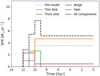 |
Fig. 1. SFR of all Galactic components as a function of lookback time. The current time is 0. The old SFR model (blue dotted line) is plotted for comparison. |
2.5.1. Galactic bulge
The Galactic bulge is the central part of the Galaxy with a corotation radius of ∼4 kpc (Gerhard et al. 2001). In our calculation we assumed that the total stellar mass of the Galactic bulge is 0.91 ± 0.07 × 10¹⁰ M⊙ (Licquia & Newman 2015). Stellar metallicity and age distribution cover a wide range of values, as is shown both by observations (e.g., Bensby et al. 2018) and cosmological simulations (e.g., Kobayashi & Nakasato 2011). To reconstruct the properties of the stellar populations in the bulge, we used the figures from Kobayashi & Nakasato (2011), for the stellar age distribution Fig. 7, and for the stellar age-metallicity relation Fig. 8.
We approximated the metallicity and age relations in the following way: half of the stars in the bulge formed 10–12 Gyr ago (a formation peak, SFR = ∼2.3 M⊙ yr−1) and the other half of the stars formed from 10 Gyr ago to the current time, with a constant SFR of ∼0.5 M⊙ yr−1. Star systems that are older than 10 Gyr were divided into four groups equal in mass, of metallicities 0.1 Z⊙, 0.3 Z⊙, 0.6 Z⊙, and 1.0 Z⊙. A stellar population younger than 10 Gyr has a high metal content, equal to 1.5 Z⊙. Our model of the star formation and metallicity for the bulge is shown in Fig. 2.
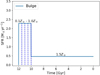 |
Fig. 2. SFR and metallicity in the Galactic bulge as a function of lookback time. The current time is 0. Vertical dashed lines separate stellar populations with different metallicities. |
2.5.2. Galactic disk
In our calculations we used the total mass of the Galactic disk, 5.17 ± 1.11 × 10¹⁰M⊙, estimated by Licquia & Newman (2015). We assumed that disk is divided into two main components, the thick and the thin disk. They had different star formation histories. The stellar populations in the disk have different metal contents and ages. The thin disk is dominant in mass; it contains about 90% of all disk stars (Cignoni et al. 2006). In our model 90% of the total disk stellar mass is therefore contained in the thin disk, and the remaining 10% of mass is in the thick disk.
The thick disk formed first, and its average age has been estimated to be 9.6 Gyr ±0.3 by Soubiran & Girard (2005). The contribution of stars younger than 9 Gyr to the thick disk is very low, as was shown by Cignoni et al. (2006). In our model the stellar population in the thick disk formed with an SFR = ∼2.5 M⊙ during the period from 11 to 9 Gyr ago and has a metal content equal to 0.25 Z⊙, see Fig. 6 (Liu et al. 2018).
The SFR of the thin disk was estimated based on the age distribution of observed stars shown in Fig. 13 in Casagrande et al. (2011) and on the results of Kobayashi & Nakasato (2011). We approximated figures by ten star formation episodes, which started 10 Gyr ago and lasted until the present moment. New episodes occurred every 1 Gyr and lasted for Δt = 1 Gyr, with the constant SFR equal to ∼5 M⊙ yr−1. Based on the metallicity-age relation presented in Haywood et al. (2013, 2015), in the next formation episodes, the metal content of the stellar populations increased and changed from 0.1 Z⊙ to Z⊙ with a rate of ΔZ = 0.1 Z⊙ Gyr−1. Our SFR and metallicity distribution model of the disk as a function of time is shown in Fig. 3.
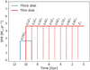 |
Fig. 3. SFR and metallicity of the Galactic disk as a function of lookback time. The current time is 0. Vertical dashed lines separate stellar populations with different metallicities. |
2.5.3. Galactic halo
The Galactic halo is the most massive Galactic component. The total mass of the halo is estimated as ∼1012 M⊙ (Wang et al. 2015; Grand et al. 2019), but most of it is dark matter, which does not reflect or emit electromagnetic radiation. In our simulation we considered only the stellar mass in the Galactic halo, which is a small fraction of the total halo mass, estimated to be about 2 × 10⁹ M⊙ (Morrison et al. 2000; Chiba & Beers 2000; Yanny et al. 2000; Siegel et al. 2002; Bullock & Johnston 2005). To reconstruct the age and metallicity of stars in the halo, we used cosmological simulations results and the figures from Kobayashi & Nakasato (2011), Fig. 7 for the distribution of stellar ages and Fig. 8 for the stellar age–metallicity relation. We simplified the relation by dividing the halo into two components equal in mass that formed 11–12 Gyr and 10–11 Gyr ago with metallicities of 0.01 Z⊙ and 0.02 Z⊙, respectively, and a SFR of ∼0.5 M⊙ yr−1. The model of the SFR and metallicity in the halo is shown in Fig. 4.
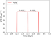 |
Fig. 4. SFR and metallicity of the Galactic halo as a function of lookback time. The current time is 0. The vertical dashed line separates stellar populations with different metallicities. |
2.6. Velocities and coordinates of Galactic BHs
In our online database3 we list simple estimates of Galcatic coordinates and BH velocities. The coordinates of the BHs were randomly selected using formulas for stellar mass distributions in Galactic components. For the bulge and halo, we used the formulas given by Korol et al. (2018). For the bulge we drew the distances to the Galactic center from the range [0–4] kpc, setting the parameter rb = 1.0 kpc (the characteristic radius of the bulge), while for halo, the possible distance range is [15–30] kpc. We assumed that both bulge and halo are spherical. For BHs in the Galactic disk we used the expression from Li (2016). We drew distances from the range of [2–15] kpc in order to obtain x and y coordinates, while the z coordinate was taken from the uniform distribution in range [−0.15,0.15] kpc because we assumed an average disk height of 0.3 kpc (Rix & Bovy 2013). Here we set the parameter rb = 2.0 kpc (the radius of the central bulge) for continuity between the disk and bulge components.
The total velocity of a Galactic BH is the sum of the motion in the Milky Way gravitational potential and the velocity obtained during isolated or binary evolution. In our estimation of the BH speed, we considered the rotation velocities around the Galactic center and additional BH velocities from physical processes such as SN explosions. Single and binary BHs might obtain a significant portion of kinetic energy after SN or core-collapse formation through a flux release of asymmetric neutrinos (Fryer et al. 2012; Janka 2017). If the BH is in a binary system, the whole system changes its velocity after the first and second NS or BH formation (Kalogera 1996). If the velocity is high enough, the binary system disrupts. The disruption of a binary system may occur not only in asymmetric SN explosions. A disruption may also be the result of a Blaauw kick (Blaauw 1961) associated with symmetric mass loss, which leads to a change in the mass ratio and in the orbital elements of the system.
We calculated the velocities of single and binary BHs after their formation in three spatial dimensions, VS = [VSx,VSy,VSz]. To estimate the motion of BHs in the Milky Way potential, we used an approximated form of the Galactic rotational curve (Vr) that has been applied in other Galactic simulations (e.g., Abramowicz et al. 2018). The simplified rotational curve has the form
In our estimates, Rb is the radius of bulge, equal to 4 kpc (Gerhard et al. 2001), and r is the distance from the BH to the Galactic center generated from the bulge mass distribution (Korol et al. 2018), as described above.
In order to calculate the sum of the two velocities (VS, Vr), we generated components of vector Vr in three spatial dimensions for the bulge and halo (spherical motion) and in two dimensions for the disk (motion in plane). The total BH velocity in our results is the norm of the sum of the two velocities VS and Vr in three dimensions.
3. Results
We present the results of our simulations for the Galactic components in Sect. 3.1 for the bulge, Sect. 3.2 for the disk (thin and thick), and in Sect. 3.3 for the halo. In each of the subsections we provide tables for single and binary BHs. The tables contain basic statistical information such as estimated number of BHs in different configurations, formation channels, and average masses of BHs and their companions (for binary BHs). The tables list two values that refer to the two evolution models A and B (see Sect. 2.3), given in the order A/(B).
In the table with single BHs we include single stars, mergers, and disrupted binaries. These sections refer to the BH formation channel. The section single stars contains BHs that are remnants of the massive single star evolution. The merger section includes single BHs created through coalescence of a binary system, and it is divided into several rows corresponding to the types of objects that have merged. The third section contains BHs from disrupted binary systems. In the merger section, the entries in the row with BH-BH systems refer to the number of single BHs that formed in the merger of two BHs, while in the section for disrupted systems, the number in the row BH-BH is the total number of single BHs after system disruption (i.e., twice the number of disrupted BH-BH binaries).
The table with binary system BHs contains two sections: one with DCO systems (BH-BH, BH-NS, and BH-WD), and one with other binary systems in which the BH companion is an unevolved star. The table contains information about the types of the BH companion objects, the estimated number of BHs in a given Galactic component, and their average masses.
In Sect. 3.4 we constrain the amount of dark matter that might be hidden in the Galactic halo in the form of stellar origin BHs, which cannot be detected by current observation surveys.
In Sect. 3.10 we calculate the change in Galactic CO merger rates from the Milky Way formation until the present time. In Table 2 we present the current Galactic merger rates for BH-BH, BH-NS, and NS-NS binary systems. In Sect. 3.5 we present and discuss the distribution of single and binary BH mass in the Galactic bulge, disk, and halo. In Sect. 3.7 we show and discuss the velocity distribution of single and binary BHs in the Galactic components. In Table 3 we list the average speeds of BHs in the bulge, disk, and halo. We constrain the fraction of BHs with speeds high enough to escape from the Galaxy. In Fig. 5 we show the change in the total numbers of single BHs and BHs in binary systems in the Milky Way from the Milky Way formation until the present time for the two evolutionary models A and B (Sect. 2.3).
Current Galactic merger rates for a new and old Galactic SFR and chemical evolution models.
Average values of BH speeds in the Galactic components bulge, disk, and halo.
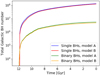 |
Fig. 5. Total number of formed Galactic BHs, single and binary, as a function of time. The current time is 0. Results for the two calculated models A and B (Sect. 2.3). |
3.1. Galactic bulge
We find that the Galactic bulge hosts about 1.7 × 10⁷ single BHs and about 1 × 10⁶ BHs in different types of binary systems. The average mass of a single BH is 11.7/(11.3) M⊙, and the average mass of a BH in a binary system is ∼15.6/(15.8) M⊙. The most massive BHs in the bulge are formed by coalescence of a massive binary system (BH and a massive star or binary BH system), and they can reach ∼100 M⊙.
A significant number of single BHs in the bulge (nearly 50%) are remains of the evolution of single massive stars. The average mass of such a BH is ∼11.7 M⊙. The second important origin of single BHs is a merger of a binary system, especially MS-MS and MS-He. Almost 30% of the single BHs in the bulge are formed in mergers, and their remaining masses cover a wide range of values. The least massive single BHs originates from mergers of low-mass binaries such as WD-MS or WD-He. The formed masses often fill the first observational mass gap between 3–5 M⊙ (Demorest et al. 2010; Antoniadis et al. 2013; Swihart et al. 2017; Wyrzykowski & Mandel 2020). The third main formation channel of single BHs is the disruption of binary systems after formation of a BH or NS. These BHs are about 20% of all single BHs in the bulge, and their average mass is ∼10 M⊙.
The average BH mass in a binary system is ∼17 M⊙. Most binary systems with a BH in the bulge are BH-BH systems (80% of the binary BHs). The BHs in binary systems with a noncompact companion make up about 3% of all binary BHs in the bulge.
3.2. Galactic disk
About 80% of Galactic BHs are in the disk because in our simulation, this is the most massive component (see Sect. 2.5). In the two disk components, the thin and thick disk, there are in total ∼1.0 × 10⁸ single BHs with an average mass of ∼14 M⊙ and about ∼8 × 10⁶ BHs in binary systems with an average mass of BH ∼19 M⊙. The most massive BHs in the Galactic disk have a mass of ∼100 M⊙, and they are formed by coalescence of a BH and a massive star (MS or He).
There are three main formation channels of single BHs in the Galactic disk. About 45% of the single BHs in the thin disk and in thick disk are final remnants of the evolution of massive single stars. The second important channel is the merger of binary systems, which leads to the formation of 25–30% of single BHs in the disk. The BHs from disrupted binaries make up about 20% of all single BHs in the disk, and their average mass is ∼12 M⊙.
Most binary BHs in the disk (∼80% of BHs in binaries) are in a BH-BH configuration. The average mass of a BH in a binary system is about ∼19 M⊙. The fraction of BHs with an unenvolved companion is small, lower than 2% of all binary BHs in the disk.
3.3. Galactic halo
The Galactic halo is the least massive component in our simulation because we considered only its stellar mass (Sect. 2.5). Most of the halo mass is not in stars, therefore we did not consider this mass in the stellar origin BH formation. The total number of BHs in the halo is only 4% of the entire Galactic BH population, it contains ∼4 × 10⁶ single BHs with an average mass ∼20 M⊙ and about ∼5 × 10⁵ BHs in binary systems with an average BH mass ∼24 M⊙.
Because the metallicity of the stellar populations is low, the most massive BH in the simulations, with a mass of 113 M⊙, is formed in halo. It originates from a merger of a BH and a He star. The formation channels of single BHs in the halo are the same as in the disk and bulge. Over 50% of single BHs are remnants of the evolution of single massive star, and 20–25% formed in binary system mergers (mainly MS+MS, MS+He, and WD+He). The BHs from disrupted binary systems make up ∼15% of the single BHs in the halo, and have an average mass of about 17 M⊙.
3.4. Dark matter in BHs of stellar origin
Several microlensing surveys have been made towards the halo in order to search for and constrain the number of massive compact halo objects (MACHOs) that may constitute part of the dark matter (Alcock et al. 2001). MACHOs with masses over 20 M⊙ cannot be excluded by observations (Tisserand et al. 2007; Wyrzykowski et al. 2011) because current microlensing surveys do not cover timescale that are long enough to detect such massive objects. On the other hand, the existence of wide binary systems in the halo indicates the absence of MACHOs with masses higher than ∼100 M⊙. The observed binaries would likely disrupt in interaction with objects with such a high mass (Yoo et al. 2004; Monroy-Rodríguez & Allen 2014). These two restrictions give us the most recent upper and lower limit on the MACHO mass range (Bird et al. 2016).
We calculated the fraction of mass in the Galactic halo that is hidden in the form of stellar origin BHs in the mass range of 20–100 M⊙. The total mass of such BHs is ∼6.2 × 10⁷M⊙, which could constitute only ∼0.006% of the total Galactic dark matter mass, which is ∼1012 M⊙ (Wang et al. 2015; Monari et al. 2018; Grand et al. 2019).
3.5. Mass distribution
In Figs. 6 and 7 we present the distribution of single and binary BHs masses for the two evolutionary models A and B and the three Galactic components bulge, disk, and halo. The mass distribution for single and binary BHs is very different. The average mass of a BH in a binary system ∼19 M⊙ is higher than for single BHs with an average mass of ∼14 M⊙. The difference in average mass of single and binary BHs is mainly due to the distribution of our adopted natal kick: the less massive the remnant (BH or NS), the higher the velocity it obtains. This results in the disruption of many low-mass binaries during the formation of a BH or NS. In all Galactic components, the mean BH mass in a binary BH-BH system is higher than the mass of a BH from distrupted BH-BH systems (see Tables 4–11). Moreover, BHs in a binary system are mainly in BH-BH systems because of the distribution of the natal kick we assumed (80% of the Galactic binary BHs).
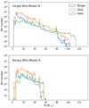 |
Fig. 6. Single (top) and binary (bottom) BHs mass distribution in the three Galactic components for model A. In model A we allowed a binary system to survive the CE phase with an HG donor star. The mass of the objects formed in a merger is estimated as explained in Sect. 2.4. |
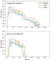 |
Fig. 7. Single (top) and binary (bottom) BHs mass distribution in the three Galactic components for model B. In model B we assumed that the CE phase with an HG star donor always leads to a binary system merger. The mass of the objects that formed in a merger is estimated as explained in Sect. 2.4. |
Single BHs in the bulge.
Binary systems with BHs in the bulge.
Single BHs in the thin disk.
Single BHs in the thick disk.
Binary systems with BHs in the thin disk.
Binary systems with BHs in the thick disk.
Single BHs in the halo.
Binary systems with BHs in the halo.
The distributions of single BH masses in all Galactic components (disk, bulge, and halo) peak near 10–15 M⊙, and above this mass, the number of BHs systematically decreases and reaches zero at different mass limits depending on the Galactic component (note the log scale). In the halo, the decrease in number of BHs along with the mass is fainter than in the bulge or disk. The average single BH mass in the halo (∼17 M⊙) is higher than in the other components (bulge and disk ∼12–13 M⊙). The occurrence of more massive BHs is due to the lower stellar metallicity (Belczynski et al. 2010), which is associated with less weight loss from massive stars through stellar winds. The range of possible single BH masses (∼2.5–113 M⊙) is wide because a significant number of single BHs originates from binary system mergers (∼20–30%), which might be both low (the final BH mass close to the highest NS limit) and high mass. The average mass of BHs of all merger types is similar to other formation channels. However, BHs from mergers widen the range of possible BH masses above the PPSN limit and fill the first and second mass gap (merger of a massive BH with its binary companion). The first mass gap (Demorest et al. 2010; Antoniadis et al. 2013; Swihart et al. 2017) between 3–5 M⊙.is filled by BH masses that mainly formed by coalescence of WD and He or MS stars. We assume that a merger of a WD and a massive star leads to the collapse to a BH or NS. As we mentioned before, single BHs are hard to detect, therefore BHs in the mass gap do not contradict observations (Wyrzykowski & Mandel 2020). The second mass gap is mainly filled by mergers of BH+He, BH+MS stars, and BH-BH. In the bulge and disk, the highest achieved BH mass is ∼100 M⊙, and in the halo it is over 110 M⊙.
To determine the effect of the criterion we adopted for estimating the masses of objects formed in mergers (e.g., the formation of objects in the first and second mass gaps), we tested two alternative simplified methods. In the first method we set factors that defined the fraction of the accreted mass of the merging companion (see fMS, fG, andfHe Sect. 2.4) to zero, that is, we did not allow for accretion from the second object. In the second method, the factors were set to 0.5, that is, we assumed accretion of one half of the mass of the companion. For DCO mergers we made an exception and took the sum of merging objects without any mass loss. The distribution of BH masses for the nonaccretion and half-accretion cases for the two CE models A and B are shown in Figs. 8–11.
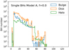 |
Fig. 8. Single BH mass distribution in the three Galactic components for model A. In model A we allowed a binary system to survive the CE phase with an HG donor star. The mass of the objects that formed in a merger is estimated as a lower limit assuming total mass loss from the second merging object (except for two CO mergers). |
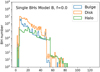 |
Fig. 9. Single BH mass distribution in the three Galactic components for model B. In model B we assumed that the CE phase with an HG star donor always leads to a binary system merger. The mass of the objects thata formed in merger is estimated as a lower limit assuming total mass loss from the second merging object (except for two CO mergers). |
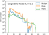 |
Fig. 10. Single BH mass distribution in the three Galactic components for model A. In model A we allowed a binary system to survive the CE phase with an HG donor star. The mass of the objects that formed in a merger is shown, assuming 50% mass loss from the second merging object (except for two CO mergers). |
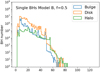 |
Fig. 11. Single BH mass distribution in the three Galactic components for model B. In model B we assumed that the CE phase with an HG star donor always leads to a binary system merger. The mass of the objects that formed in a merger is shown, assuming 50% mass loss from the second merging object (except for two CO mergers). |
In general, the use of different methods did not have a strong effect on the average single BH masses in the Galactic components, especially considering evolutionary model B. However, a significant reduction in the number of low-mass BHs below 5 M⊙(first mass gap) in the results for the nonaccretion model (f = 0.0, Figs. 8 and 9) is clear. In the three tested models (standard, f = 0.0, and f = 0.5), both mass gaps are filled by the products of mergers. However, the number of BHs in first and second mass gap strongly depends on the assumed accretion factor f. In the nonaccretion model, objects in the second mass gap are only products of DCO mergers, and in the other two models, BHs with masses higher than the PPSN limit might have formed, for example, by a BH and MS or BH and HE star coalescence. The average single BH masses for the three tested mass estimates are given in the Table 12. Because accretion of matter during merger is reduced, the total number of single BHs is lower the smaller the accretion factor f. The total number of single BHs was reduced by about 20% for the nonaccretion model and about 1% for the model with half-accretion compared to our standard model described in Sect. 2.4.
Average single BH masses in the Galactic components bulge, disk, and halo.
The binary BHs in the halo are also mainly in BH-BH binaries (∼80% of the binary BHs). The fraction of BHs with a noncompact companion in the halo is ∼1.5%.
The range of possible binary BH masses is narrower than for single BHs. The upper limit on binary BHs mass (∼50–60 M⊙) is similar in all Galactic components, disk, bulge, and halo, and it is the result of two physical processes: stellar winds (Belczynski et al. 2010) and the pair-instability limit (Woosley 2017; Leung et al. 2019). The upper limit is consistent with the second observational mass gap. The first mass gap is also reconstructed for binary BHs in the rapid SN model (Fryer et al. 2012). However, there is a narrow, isolated peak near a range of 2.5–3 M⊙ (close to the highest NS mass). The peak is made of BHs that formed in accretion of matter on the massive NS from its binary companion. The fraction of BHs with an unevolved companion (e.g., MS or G star) is small, a few percent of all binary BHs. The companion is usually a low-mass star M < 1 M⊙. More massive stars are less frequent, especially in older stellar populations, becaue their evolution time is shorter than most population ages. Even if the NS interacts with the more massive companion, the mass transfer onto the NS or BH during a short-lived CE event is related to the Bondi-Hoyle accretion, which in our model is rather inefficient (see Sect. 2).
3.6. Separation and eccentricity of BH binary systems
In our database we include orbital parameters (separation and eccentricity) of all binary systems that contain a BH. The distribution of the system separation in the Galactic components for the CE model A (top) and B (bottom) is plotted in Fig. 12 (log-log scale) and covers a wide range from a few R⊙ to 108R⊙. The average separation is different in the Galactic components: in the bulge, it is ∼8.8 × 10⁴(9.4 × 10⁴) R⊙, in the disk, it is ∼6.4 × 10⁴(7.4 × 10⁴) R⊙ , and in the halo, it is ∼3.9 × 10⁴(3.9 × 10⁴) R⊙.
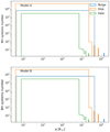 |
Fig. 12. Distribution of the separation in all Galactic BH binary systems in the three Galactic components and for CE models A (top) and B (bottom). |
The distribution of the BH system eccentricities in the Galactic components is shown in Fig. 13 for model A (top) and model B (bottom). It is dominated by low eccentricities, with a high peak near 0–0.1. The average eccentricity of BH binary systems is similar in all Galactic components and is in the range of [0.15−0.18]. The components in wide binary systems did not exchange mass during the evolution, and the orbit was only affected by wind mass loss, magnetic braking, or emission from gravitational waves.
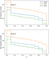 |
Fig. 13. Distribution of the eccentricity in all Galactic BH binary systems in the three Galactic components and for CE models A (top) and B (bottom). |
3.7. Velocity
In Figs. 14 and 15 we plot the distribution of the velocities of a single and a binary BH for the two models A and B (see Sect. 2.3) and the three Galactic components. With the red dashed line we mark the velocity equal to 580 km s−1, which is the estimated value of the local Galactic escape speed at the position of the Sun (Monari et al. 2018). The escape speed depends on the location in the Milky Way and can take values in the range from ∼550–650 km s−1.
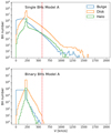 |
Fig. 14. Single (top) and binary (bottom) BHs velocity distribution in the three Galactic components for model A. In model A we allowed a binary system to survive the CE phase with an HG donor star. With the red dashed line we mark the velocity equal to 580 km s−1, which is the estimated value of the local Galactic escape speed at the position of the Sun (Monari et al. 2018). |
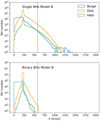 |
Fig. 15. Single (top) and binary (bottom) BHs velocity distribution in the three Galactic components for model B. In model B we assumed that the CE phase with an HG donor star always leads to a binary system merger. With the red dashed line we mark the velocity equal to 580 km s−1, which is the estimated value of the local Galactic escape speed at the position of the Sun (Monari et al. 2018). |
The average value for single and binary BHs is similar in a given Galactic component because BHs in general do not reach high speeds as a result of the binary or single evolution. Most BH velocities are close to the values that we adopted from the approximated form of the rotation curve for a given component (Sect. 2 or Sect. 2.6). Very high speeds of single BHs (over 1000 km s−1) are rare cases (note the log scale). However, there is a difference in the range of possible speeds of single and binary BHs. Single BHs may achieve speeds from 0 to even ∼1700 km s−1 in model A and to 1100 km s−1 in model B. The maximum speed of a BH in a binary system is ∼700 km s−1. This is a result of the natal kick distribution we assumed (see Sect. 2). An NS and a low-mass BHs receive higher natal kicks, inversely proportional to the remnant mass. These systems are often disrupted. BHs from disrupted binaries may achieve high velocities and are classified as single BHs. BHs in binary systems are often more massive and receive lower natal kicks (remain bound). Sporadic cases of very high speeds in model A are low-mass BHs from close binaries that became disrupted after the formation of the BH or NS that passed CE phase with an HG donor. In the Table 3 we present the average single and binary BH speeds for the two models A and B and the Galactic bulge, disk, and halo.
We calculate that ∼5% of the single BHs (∼6 × 10⁶) and less than 0.0001% of the binary BHs (∼10) have velocities greater than 550 km s−1, the lowest escape velocity from the Milky Way (Monari et al. 2018). This gives us an upper limit on the fraction of BHs that might escape form the Galaxy in our physical model. If we were to adopt a natal kick model with no fallback parameter, the fraction of BHs with very high velocities would increase.
3.8. BH binaries with a noncompact companion
We present the parameters of our synthetic population of Galactic BHs with a nonevolved binary companion, which might be an MS, G, or He star. This fraction of BH systems might be especially interesting for BH hunters because these systems are more likely to be detected because they have a visible companion. However, they appaer to make up only a small fraction (less than 1% of all Galactic BHs).
In Figs. 16 and 17 we plot the mass distribution of BHs (top) and their companions (bottom) for the two CE models A and B and the three Galactic components. The mass distribution is similar for models A and B, and the mass distribution for BHs and their companions varies depending on the given Galactic component. The mean masses of the BHs in the Galactic components are ∼16 M⊙ in the disk, ∼11 M⊙ in the bulge, and ∼21 M⊙ in the halo, while the mean masses of the companion stars are ∼3.5 M⊙ in the disk, ∼2.0 M⊙ in the bulge, and ∼0.5 M⊙ in the halo. The differences in BH masses are mainly the effect of the metallicity, which is very low in the halo compared with the disk and bulge. The difference in the companion mass distribution is the result of the age and star formation history of a given component. We assumed that stellar populations in the halo formed 10–12 Gyr ago, which means that only low-mass stars have not yet completed their evolution. On the other hand, we assumed that many young stars are located in the disk and some young populations in the bulge, so that binaries with more massive stars are still possible. We plot the orbital parameters (separation and eccentricity) of the systems. The distribution of the separations is shown in Fig. 18 and the eccentricities in Fig. 19. The distribution of the separations covers a wide range from a few R⊙ to 107R⊙ and appears to be approximately uniform on the log-log scale. The eccentricities of the systems are rather low; there is a peak in the number of systems with eccentricities 0–0.1, while the average of all Galactic components is about 0.25. In Fig. 20 we plot a diagram that illustrates the relationship between the system separations and eccentricities.
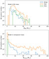 |
Fig. 16. Distribution of a BH (top) and its companion masses (bottom) in Galactic BH binary systems with a nonevolved companion in the three Galactic components for evolution model A. |
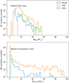 |
Fig. 17. Distribution of a BH (top) and its companion masses (bottom) in Galactic BH binary systems with a nonevolved companion in the three Galactic components for evolution model B. |
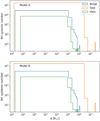 |
Fig. 18. Distribution of the separation in Galactic BH binary systems with a nonevolved companion in the three Galactic components for evolution models A (top) and B (bottom). |
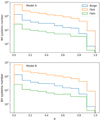 |
Fig. 19. Distribution of the eccentricity in Galactic BH binary systems with a nonevolved companion in the three Galactic components for evolutionary models A (top) and B (bottom). |
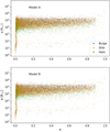 |
Fig. 20. Diagram with orbital parameters. The separation and eccentricity for BH binary systems with a noncompact companion. Results for the two models A (top) and B (bottom) are shown. |
3.9. Massive BHs from MS+He mergers
We found some cases of MS+He star mergers that can produce a star with a He core mass below the pair-instability limit, with a total mass (core + envelope) as high as 60–90 M⊙. We assumed that the naked He star is more compact than a MS star, and therefore the mass of the core after a merger would not increase. This means that the total mass accreted from the MS companion creates the envelope. It has been shown by Woosley (2017) that for ultralow-metallicity and Population III stars the PPSN or PSN instability can be shifted to ∼70 M⊙ at most because such stars can keep massive H-rich envelopes. Considering this limit, we removed from our database BHs that formed in an MS+He merger that are more massive than 70 M⊙. However, single BHs with masses above that limit can be still created in BH mergers, for instance, BH+MS or BH+BH mergers. A similar scenario was recently considered by Tanikawa et al. (2019) in the context of LB-1 formation.
3.10. Galactic merger rates
We calculated the change in merger rates of DCO systems (BH-BH, BH-NS, and NS-NS) from the Galactic formation until the present. We present results for the two models A and B (Sect. 2.3). The DCO merger rates have changed along with the star formation and stellar metallicity of the Galactic components (see Fig. 21). In general, the higher the SFR at the given time, the higher the merger rates because the time-delay distribution between the formation of a binary system and its merger is a steep power law (∝t−1) (Dominik et al. 2012). Furthermore, the metallicty of the stellar population is an important factor that strongly influences the DCO merger rates, especially for BH-BH systems (Dominik et al. 2013; Spera et al. 2015; Dvorkin et al. 2016). The highest BH-BH merger rates in models A and B occurred between 8–11 Gyr ago. The effect was caused by a peak in SFR (Sect. 2.5) because at that time the star formation episode in bulge intensified, the stellar population of the thick disk formed, and the star formation in the thin disk had started. High BH-BH merger rates were also caused by the low metallicity of the stars that formed in this period. In both models the BH-BH merger rates decrease with time, but in model B the rates decrease more dramatically. At higher metallicity, binary systems evolve in a such way that the HG star is more often a donor in the CE phase because of increased mass loss through stellar winds. These systems are then eliminated from a binary system population (see Sect. 2.3).
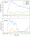 |
Fig. 21. Merger rates of DCO binaries (BH-BH, BH-NS, and NS-NS) as a function of time since the Big Bang. Results are shown for a new Galactic SFR and chemical evolution model (Sect. 2.5) and for the two evolutionary models A and B, see Sect. 2.3. Current time is 0. |
The merger rates of BH-NS and NS-NS systems did not change so much with Galaxy formation and metallicity as the rates for BH-BH systems. A lower metallicity slightly decreases the NS-NS merger rates, but this effect was compensated for by more intensive SFR episodes at early ages (8–11 Gyr). Because in the standard physical model we assumed natal kicks with high σ = 265 km s−1 (see Sect. 2.2) and a fallback factor inversely proportional to the mass, many low-mass CO binary systems become disrupted by SN explosion or core collapse. These disruptions decreased the CO merger rates, especially for NS-NS systems. Our rates for DCO system mergers can be compared with the results for other implemented physical models for a wide range of natal kick distributions, CE efficiency parameters, or the mass fraction that is ejected during RLOF, which are presented in for example: Tutukov et al. (1992), Abadie et al. (2010), Voss & Tauris (2003), Belczynski et al. (2018).
For comparison, we present the evolution of the merger rates and the current values for an old simplified Galactic SFR and for a chemical evolution model (Fig. 22). The previous model assumed only one Galactic component (disk) with mass 3.5 × 10¹⁰ M⊙. The SFR was constant during 10 Gyr (3.5 M⊙ yr−1), and all stars were formed with the same metallicity equal to Z⊙ = 0.014.
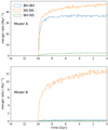 |
Fig. 22. Merger rates of DCO binaries (BH-BH, BH-NS, and NS-NS) as a function of time since the Big Bang. Results are shown for an old Galactic SFR and a chemical evolution model and the two evolutionary models A and B, see Sect. 2.3. Current time is 0. |
In Table 2 we present the current Galactic merger rates of BH-BH, BH-NS, and NS-NS systems per Myr−1 for the two CE models A and B. For comparison we also calculated the current merger rates for an old SFR and for the metallicity distribution model of the Milky Way (Sect. 2.5). Merger rates for the old model are in general lower than for the new model for all types of DCO systems. The most significant difference is in the case of BH-BH systems, for which current rates (in model B) are one order of magnitude lower for the old model.
We calculated the fractions of current Galactic DCO systems that will merge in one Hubble time (in the next 14 Gyr). The percentage fraction of such systems for the two evolution models is given in the order A/(B), ∼6%/(1%) for BH-BH, ∼13%/(6%) for NS-NS, and ∼16%/(2%) for BH-NS systems. Star formation is still taking place in some parts of the Milky Way, therefore the number of DCO systems will also increase. Numerical data are presented in Table 13.
Number of current Galactic double compact systems that will merge in a shorter and longer time than the Hubble time (THub).
We do not compare our current Galactic results with LIGO/Virgo estimates because to calculate the cosmic merger rate of a DCO, the entire cosmic SFR(z) and metallicity distribution Z(z) as a function of redshift need to be considered. However, this calculation for StarTrack physical models (including those presented in this work) were carried out in Belczynski et al. (2017), Sect. 3.2, noting full agreement with BH-BH, BH-NS, and NS-NS LIGO/Virgo estimates.
4. Conclusions
We presented population synthesis statistical estimates of the current Milky Way BH population properties. We used the most recent version of the code StarTrack with standard physics (Sect. 2) and processed the data with the new SFR and metallicity distribution model of our Galaxy, based on theoretical models and observations. We showed results for two models A and B, which correspond to different scenarios of a CE phase (Sect. 2.3). Our results are listed below.
(1) At the present moment, the Milky Way (disk+bulge+halo) contains about 1.2 × 10⁸ single BHs with an average mass 14 M⊙ and 9.3 × 10⁶ BHs in binary systems with an average mass 19 M⊙.
(2) There are three main formation channels of single BHs: ∼50% are remnants of massive single star evolution, ∼30% formed in binary system mergers, and ∼20% of the single BHs originate in disrupted binary systems during the formation of a BH or neutron star.
(3) The most massive BH in the simulation comes from the old low-metal environment of the Galactic halo. It formed by BH-MS system coalescence, and its mass is as high as ∼113 M⊙.
(4) BHs in binary systems constitute ∼10% of the whole Galactic BH population. Most of the BHs in binary systems are in a BH-BH configuration. The fraction of BH binaries with noncompact companion is small, about 0.3% of all Galactic BHs.
We estimated the change in the merger rates of DCO systems (BH-BH, BH-NS, and NS-NS) along with the Galaxy star formation. The current Galactic merger rates depend on the model, and they are estimated at ∼81/3 Myr−1 for BH-BH, ∼9/1 Myr−1 for BH-NS, and ∼59/14 Myr−1 for NS-NS systems.
(5) We constrain that only ∼0.006% of the total Galactic halo mass (including dark matter) could be hidden in the form of BHs with stellar origin, which cannot be detected by current observational surveys.
(6) The velocities of only ∼5% of the single BHs and 0.001% of the binary BHs are high enough to escape from the Galactic potential.
Because of our assumption of the binary fraction Sect. (2.2) and orbital seperation (Sect. 2.1), the number of binary systems and system mergers might be slightly underestimated.
https://stellarcollapse.org/sites/default/files/table.pdf and references within.
https://stellarcollapse.org/sites/default/files/table.pdf and references within.
Acknowledgments
Authors acknowledge support from the Polish National Science Center (NCN) grant: project Maestro 2018/30/A/ST9/00050 We would like to thank: Grzegorz Wiktorowicz, Pawel Pietrukowicz and Thomas Bensby for their comments and advices.
References
- Abadie, J., Abbott, B. P., Abbott, R., et al. 2010, CQG, 27, 173001 [Google Scholar]
- Abbott, B. P., Abbott, R., Abbott, T. D., et al. 2016a, Phys. Rev. X, 6, 041015 [Google Scholar]
- Abbott, B. P., Abbott, R., Abbott, T. D., et al. 2016b, Phys. Rev. Lett., 116, 241103 [Google Scholar]
- Abbott, B. P., Abbott, R., Abbott, T. D., et al. 2016c, Phys. Rev. Lett., 116, 061102 [Google Scholar]
- Abbott, B. P., Abbott, R., Abbott, T. D., et al. 2017a, Phys. Rev. Lett., 118, 221101 [NASA ADS] [CrossRef] [PubMed] [Google Scholar]
- Abbott, B. P., Abbott, R., Abbott, T. D., et al. 2017b, ApJ, 851, L35 [NASA ADS] [CrossRef] [Google Scholar]
- Abbott, B. P., Abbott, R., Abbott, T. D., et al. 2017c, Phys. Rev. Lett., 119, 141101 [NASA ADS] [CrossRef] [PubMed] [Google Scholar]
- Abramowicz, M. A., Bejger, M., & Wielgus, M. 2018, ApJ, 868, 17 [CrossRef] [Google Scholar]
- Alcock, C., Allsman, R. A., Alves, D. R., et al. 2001, ApJS, 136, 439 [NASA ADS] [CrossRef] [Google Scholar]
- Antoniadis, J., Freire, P. C. C., Wex, N., et al. 2013, Science, 340, 448 [Google Scholar]
- Antonini, F., Toonen, S., & Hamers, A. S. 2017, ApJ, 841, 77 [NASA ADS] [CrossRef] [Google Scholar]
- Arca-Sedda, M., Li, G., & Kocsis, B. 2018, MNRAS, submitted [arXiv:1805.06458] [Google Scholar]
- Asplund, M., Grevesse, N., Sauval, A. J., & Scott, P. 2009, ARA&A, 47, 481 [NASA ADS] [CrossRef] [Google Scholar]
- Belczynski, K., Kalogera, V., & Bulik, T. 2002, ApJ, 572, 407 [NASA ADS] [CrossRef] [Google Scholar]
- Belczynski, K., Kalogera, V., Rasio, F. A., et al. 2008, ApJS, 174, 223 [NASA ADS] [CrossRef] [Google Scholar]
- Belczynski, K., Bulik, T., Fryer, C. L., et al. 2010, ApJ, 714, 1217 [NASA ADS] [CrossRef] [Google Scholar]
- Belczynski, K., Heger, A., Gladysz, W., et al. 2016, A&A, 594, A97 [NASA ADS] [CrossRef] [EDP Sciences] [Google Scholar]
- Belczynski, K., Klencki, J., Fields, C. E., et al. 2017, The evolutionary roads leading to low effective spins, high black hole masses, and O1/O2 rates of LIGO/Virgo binary black holes [Google Scholar]
- Belczynski, K., Bulik, T., Olejak, A., et al. 2018, ArXiv e-prints [arXiv:1812.10065] [Google Scholar]
- Belczynski, K., Klencki, J., Meynet, G., et al. 2020, A&A, 636, A104 [CrossRef] [EDP Sciences] [Google Scholar]
- Bensby, T., Feltzing, S., Gould, A., et al. 2018, in Rediscovering Our Galaxy, eds. C. Chiappini, I. Minchev, E. Starkenburg, M. Valentini , IAU Symp., 334, 86 [Google Scholar]
- Bird, S., Cholis, I., Muñoz, J. B., et al. 2016, Phys. Rev. Lett., 116, 201301 [NASA ADS] [CrossRef] [Google Scholar]
- Blaauw, A. 1961, Bull. Astron. Inst. Netherlands, 15, 265 [NASA ADS] [Google Scholar]
- Brown, G. E., & Bethe, H. A. 1994, ApJ, 423, 659 [NASA ADS] [CrossRef] [Google Scholar]
- Bullock, J. S., & Johnston, K. V. 2005, ApJ, 635, 931 [NASA ADS] [CrossRef] [Google Scholar]
- Casagrande, L., Schönrich, R., Asplund, M., et al. 2011, A&A, 530, A138 [NASA ADS] [CrossRef] [EDP Sciences] [Google Scholar]
- Casares, J. 2007, in Black Holes from Stars to Galaxies – Across the Range of Masses, eds. V. Karas, & G. Matt, IAU Symp., 238, 3 [Google Scholar]
- Casares, J., & Jonker, P. G. 2014, Space Sci. Rev., 183, 223 [NASA ADS] [CrossRef] [Google Scholar]
- Chiba, M., & Beers, T. C. 2000, AJ, 119, 2843 [NASA ADS] [CrossRef] [Google Scholar]
- Cignoni, M., Degl’Innocenti, S., Prada Moroni, P. G., & Shore, S. N. 2006, A&A, 459, 783 [Google Scholar]
- de Mink, S. E., & Belczynski, K. 2015, ApJ, 814, 58 [NASA ADS] [CrossRef] [Google Scholar]
- Demorest, P. B., Pennucci, T., Ransom, S. M., Roberts, M. S. E., & Hessels, J. W. T. 2010, Nature, 467, 1081 [NASA ADS] [CrossRef] [PubMed] [Google Scholar]
- Dominik, M., Belczynski, K., Fryer, C., et al. 2012, ApJ, 759, 52 [NASA ADS] [CrossRef] [Google Scholar]
- Dominik, M., Belczynski, K., Fryer, C., et al. 2013, ApJ, 779, 72 [NASA ADS] [CrossRef] [Google Scholar]
- Duchêne, G., & Kraus, A. 2013, ARA&A, 51, 269 [Google Scholar]
- Dvorkin, I., Vangioni, E., Silk, J., Uzan, J.-P., & Olive, K. A. 2016, MNRAS, 461, 3877 [NASA ADS] [CrossRef] [Google Scholar]
- Eggleton, P. P., & Kiseleva-Eggleton, L. 2001, ApJ, 562, 1012 [NASA ADS] [CrossRef] [Google Scholar]
- Fryer, C. L., Belczynski, K., Wiktorowicz, G., et al. 2012, ApJ, 749, 91 [NASA ADS] [CrossRef] [Google Scholar]
- Gao, S., Liu, C., Zhang, X., et al. 2014, ApJ, 788, L37 [NASA ADS] [CrossRef] [Google Scholar]
- Gerhard, O. E. 2001, in Galaxy Disks and Disk Galaxies, eds. J. G. Funes, & E. M. Corsini, ASP Conf. Ser., 230, 21 [Google Scholar]
- Glebbeek, E., Gaburov, E., Portegies Zwart, S., & Pols, O. R. 2013, MNRAS, 434, 3497 [NASA ADS] [CrossRef] [Google Scholar]
- Grand, R. J. J., Deason, A. J., White, S. D. M., et al. 2019, MNRAS, 487, L72 [CrossRef] [Google Scholar]
- Haywood, M., Di Matteo, P., Lehnert, M. D., Katz, D., & Gómez, A. 2013, A&A, 560, A109 [NASA ADS] [CrossRef] [EDP Sciences] [Google Scholar]
- Haywood, M., Di Matteo, P., & Lehnert, M. 2015, Chemical and dynamical evolution of the Milky Way and Local Group, 3 [Google Scholar]
- Hobbs, G., Lorimer, D. R., Lyne, A. G., & Kramer, M. 2006, VizieR Online Data Catalog: J/MNRAS/360/974 [Google Scholar]
- Hurley, J. R., Pols, O. R., & Tout, C. A. 2000, MNRAS, 315, 543 [NASA ADS] [CrossRef] [Google Scholar]
- Hurley, J. R., Tout, C. A., & Pols, O. R. 2002, MNRAS, 329, 897 [NASA ADS] [CrossRef] [Google Scholar]
- Igoshev, A. P., & Perets, H. B. 2019, MNRAS, 486, 4098 [CrossRef] [Google Scholar]
- Ivanova, N., & Taam, R. E. 2004, ApJ, 601, 1058 [NASA ADS] [CrossRef] [Google Scholar]
- Janka, H. T. 2017, Neutrino-Driven Explosions, 1095 [Google Scholar]
- Kalogera, V. 1996, ApJ, 471, 352 [NASA ADS] [CrossRef] [Google Scholar]
- Kalogera, V., & Baym, G. 1996, ApJ, 470, L61 [NASA ADS] [CrossRef] [Google Scholar]
- Khokhlov, S. A., Miroshnichenko, A. S., Zharikov, S. V., et al. 2018, ApJ, 856, 158 [NASA ADS] [CrossRef] [Google Scholar]
- Klencki, J., Wiktorowicz, G., Gładysz, W., & Belczynski, K. 2017, MNRAS, 469, 3088 [NASA ADS] [CrossRef] [Google Scholar]
- Klencki, J., Moe, M., Gladysz, W., et al. 2018, A&A, 619, A77 [NASA ADS] [CrossRef] [EDP Sciences] [Google Scholar]
- Kobayashi, C., & Nakasato, N. 2011, ApJ, 729, 16 [NASA ADS] [CrossRef] [Google Scholar]
- Kobulnicky, H. A., Kiminki, D. C., Lundquist, M. J., et al. 2014, ApJS, 213, 34 [NASA ADS] [CrossRef] [Google Scholar]
- Kochanek, C. S., Adams, S. M., & Belczynski, K. 2014, MNRAS, 443, 1319 [NASA ADS] [CrossRef] [PubMed] [Google Scholar]
- Korol, V., Rossi, E. M., & Barausse, E. 2018, Constraining the Milky Way potential with Double White Dwarfs [Google Scholar]
- Kravtsov, A. V., & Gnedin, O. Y. 2005, ApJ, 623, 650 [NASA ADS] [CrossRef] [Google Scholar]
- Kroupa, P. 2002, Science, 295, 82 [NASA ADS] [CrossRef] [PubMed] [Google Scholar]
- Kroupa, P., Tout, C. A., & Gilmore, G. 1993, MNRAS, 262, 545 [NASA ADS] [CrossRef] [Google Scholar]
- Kruijssen, J. M. D., & Mieske, S. 2009, A&A, 500, 785 [NASA ADS] [CrossRef] [EDP Sciences] [Google Scholar]
- Lamberts, A., Garrison-Kimmel, S., Hopkins, P. F., et al. 2018, MNRAS, 480, 2704 [NASA ADS] [CrossRef] [Google Scholar]
- Leung, S.-C., Nomoto, K., & Blinnikov, S. 2019, ApJ, 887, 72 [NASA ADS] [CrossRef] [Google Scholar]
- Li, E. 2016, Modelling mass distribution of the Milky Way galaxy using Gaia billion-star map [Google Scholar]
- Licquia, T. C., & Newman, J. A. 2015, ApJ, 806, 96 [NASA ADS] [CrossRef] [Google Scholar]
- Linares, M., Shahbaz, T., & Casares, J. 2018, in 42nd COSPAR Scientific Assembly, COSPAR Meeting, 42, E1.10-9-18 [Google Scholar]
- Liu, J., Zhang, H., Howard, A. W., et al. 2019, Nature, 575, 618 [NASA ADS] [CrossRef] [Google Scholar]
- Liu, S., Du, C., Newberg, H. J., et al. 2018, ApJ, 862, 163 [CrossRef] [Google Scholar]
- Lombardi, J. C., Warren, J., Rasio, J. S., Sills, F. A., & Warren, A. R. 2002, ApJ, 568, 939 [NASA ADS] [CrossRef] [Google Scholar]
- Lombardi, J. C. J., Proulx, Z. F., Dooley, K. L., et al. 2006, ApJ, 640, 441 [NASA ADS] [CrossRef] [Google Scholar]
- Mennekens, N., & Vanbeveren, D. 2014, A&A, 564, A134 [NASA ADS] [CrossRef] [EDP Sciences] [Google Scholar]
- Monari, G., Famaey, B., Carrillo, I., et al. 2018, A&A, 616, L9 [NASA ADS] [CrossRef] [EDP Sciences] [Google Scholar]
- Monroy-Rodríguez, M. A., & Allen, C. 2014, ApJ, 790, 159 [NASA ADS] [CrossRef] [Google Scholar]
- Morrison, H. L., Mateo, M., Olszewski, E. W., et al. 2000, AJ, 119, 2254 [NASA ADS] [CrossRef] [Google Scholar]
- Raghavan, D., McAlister, H. A., Henry, T. J., et al. 2010, ApJS, 190, 1 [NASA ADS] [CrossRef] [EDP Sciences] [Google Scholar]
- Rix, H. W., & Bovy, J. 2013, A&ARv, 21, 61 [NASA ADS] [CrossRef] [Google Scholar]
- Sana, H., de Mink, S. E., de Koter, A., et al. 2012, Science, 337, 444 [Google Scholar]
- Sana, H., Le Bouquin, J. B., Lacour, S., et al. 2014, ApJs, 215, 15 [CrossRef] [Google Scholar]
- Shapiro, S. L., & Teukolsky, S. A. 1983, Phys. Today, 10, 89 [CrossRef] [Google Scholar]
- Siegel, M. H., Majewski, S. R., Reid, I. N., & Thompson, I. B. 2002, ApJ, 578, 151 [NASA ADS] [CrossRef] [Google Scholar]
- Soubiran, C., & Girard, P. 2005, A&A, 438, 139 [NASA ADS] [CrossRef] [EDP Sciences] [Google Scholar]
- Spera, M., Mapelli, M., & Bressan, A. 2015, MNRAS, 451, 4086 [NASA ADS] [CrossRef] [Google Scholar]
- Swihart, S. J., Strader, J., Johnson, T. J., et al. 2017, ApJ, 851, 31 [NASA ADS] [CrossRef] [Google Scholar]
- Tanikawa, A., Kinugawa, T., Kumamoto, J., & Fujii, M. S. 2019, PASJ, submitted [arXiv:1912.04509] [Google Scholar]
- The LIGO Scientific Collaboration, & The Virgo Collaboration 2019, Phys. Rev. X, 9, 031040 [Google Scholar]
- Thompson, T. A., Kochanek, C. S., Stanek, K. Z., et al. 2019, Science, 366, 637 [NASA ADS] [CrossRef] [Google Scholar]
- Timmes, F. X., Woosley, S. E., & Weaver, T. A. 1996, ApJ, 457, 834 [NASA ADS] [CrossRef] [Google Scholar]
- Tisserand, P., Le Guillou, L., Afonso, C., et al. 2007, A&A, 469, 387 [NASA ADS] [CrossRef] [EDP Sciences] [Google Scholar]
- Tsuna, D., Kawanaka, N., & Totani, T. 2018, MNRAS, 477, 791 [CrossRef] [Google Scholar]
- Tutukov, A. V., Yungelson, L. R., & Iben, I., Jr 1992, ApJ, 386, 197 [NASA ADS] [CrossRef] [Google Scholar]
- Tylenda, R., & Kamiński, T. 2016, A&A, 592, A134 [NASA ADS] [CrossRef] [EDP Sciences] [Google Scholar]
- van den Heuvel, E. P. J. 1992, Endpoints of Stellar Evolution: The Incidence of Stellar Mass Black Holes in the Galaxy, Tech. Rep. [Google Scholar]
- Vanbeveren, D., & Donder, E. D. 2010, New Astron. Rev., 54, 50 [CrossRef] [Google Scholar]
- Voss, R., & Tauris, T. M. 2003, MNRAS, 342, 1169 [NASA ADS] [CrossRef] [Google Scholar]
- Wang, W., Han, J., Cooper, A. P., et al. 2015, MNRAS, 453, 377 [NASA ADS] [CrossRef] [Google Scholar]
- Webbink, R. F. 1984, ApJ, 277, 355 [NASA ADS] [CrossRef] [Google Scholar]
- Wiktorowicz, G., Wyrzykowski, Ł., Chruslinska, M., et al. 2019, ApJ, 885, 1 [CrossRef] [Google Scholar]
- Woosley, S. E. 2017, ApJ, 836, 244 [NASA ADS] [CrossRef] [Google Scholar]
- Wyrzykowski, Ł., & Mandel, I. 2020, A&A, 636, A20 [NASA ADS] [CrossRef] [EDP Sciences] [Google Scholar]
- Wyrzykowski, L., Skowron, J., Kozłowski, S., et al. 2011, MNRAS, 416, 2949 [NASA ADS] [CrossRef] [EDP Sciences] [Google Scholar]
- Wyrzykowski, Ł., Kostrzewa-Rutkowska, Z., & Rybicki, K. 2016a, in 37th Meeting of the Polish Astronomical Society, eds. A. Różańska, & M. Bejger, 3, 121 [Google Scholar]
- Wyrzykowski, Ł., Kostrzewa-Rutkowska, Z., Skowron, J., et al. 2016b, MNRAS, 458, 3012 [NASA ADS] [CrossRef] [Google Scholar]
- Yanny, B., Newberg, H. J., Kent, S., et al. 2000, ApJ, 540, 825 [NASA ADS] [CrossRef] [Google Scholar]
- Yoo, J., Chanamé, J., & Gould, A. 2004, ApJ, 601, 311 [NASA ADS] [CrossRef] [Google Scholar]
All Tables
Types of objects that originated from different types of stellar mergers based on Table 2 from Hurley et al. (2002).
Current Galactic merger rates for a new and old Galactic SFR and chemical evolution models.
Number of current Galactic double compact systems that will merge in a shorter and longer time than the Hubble time (THub).
All Figures
|
Fig. 1. SFR of all Galactic components as a function of lookback time. The current time is 0. The old SFR model (blue dotted line) is plotted for comparison. |
| In the text | |
|
Fig. 2. SFR and metallicity in the Galactic bulge as a function of lookback time. The current time is 0. Vertical dashed lines separate stellar populations with different metallicities. |
| In the text | |
|
Fig. 3. SFR and metallicity of the Galactic disk as a function of lookback time. The current time is 0. Vertical dashed lines separate stellar populations with different metallicities. |
| In the text | |
|
Fig. 4. SFR and metallicity of the Galactic halo as a function of lookback time. The current time is 0. The vertical dashed line separates stellar populations with different metallicities. |
| In the text | |
|
Fig. 5. Total number of formed Galactic BHs, single and binary, as a function of time. The current time is 0. Results for the two calculated models A and B (Sect. 2.3). |
| In the text | |
|
Fig. 6. Single (top) and binary (bottom) BHs mass distribution in the three Galactic components for model A. In model A we allowed a binary system to survive the CE phase with an HG donor star. The mass of the objects formed in a merger is estimated as explained in Sect. 2.4. |
| In the text | |
|
Fig. 7. Single (top) and binary (bottom) BHs mass distribution in the three Galactic components for model B. In model B we assumed that the CE phase with an HG star donor always leads to a binary system merger. The mass of the objects that formed in a merger is estimated as explained in Sect. 2.4. |
| In the text | |
|
Fig. 8. Single BH mass distribution in the three Galactic components for model A. In model A we allowed a binary system to survive the CE phase with an HG donor star. The mass of the objects that formed in a merger is estimated as a lower limit assuming total mass loss from the second merging object (except for two CO mergers). |
| In the text | |
|
Fig. 9. Single BH mass distribution in the three Galactic components for model B. In model B we assumed that the CE phase with an HG star donor always leads to a binary system merger. The mass of the objects thata formed in merger is estimated as a lower limit assuming total mass loss from the second merging object (except for two CO mergers). |
| In the text | |
|
Fig. 10. Single BH mass distribution in the three Galactic components for model A. In model A we allowed a binary system to survive the CE phase with an HG donor star. The mass of the objects that formed in a merger is shown, assuming 50% mass loss from the second merging object (except for two CO mergers). |
| In the text | |
|
Fig. 11. Single BH mass distribution in the three Galactic components for model B. In model B we assumed that the CE phase with an HG star donor always leads to a binary system merger. The mass of the objects that formed in a merger is shown, assuming 50% mass loss from the second merging object (except for two CO mergers). |
| In the text | |
|
Fig. 12. Distribution of the separation in all Galactic BH binary systems in the three Galactic components and for CE models A (top) and B (bottom). |
| In the text | |
|
Fig. 13. Distribution of the eccentricity in all Galactic BH binary systems in the three Galactic components and for CE models A (top) and B (bottom). |
| In the text | |
|
Fig. 14. Single (top) and binary (bottom) BHs velocity distribution in the three Galactic components for model A. In model A we allowed a binary system to survive the CE phase with an HG donor star. With the red dashed line we mark the velocity equal to 580 km s−1, which is the estimated value of the local Galactic escape speed at the position of the Sun (Monari et al. 2018). |
| In the text | |
|
Fig. 15. Single (top) and binary (bottom) BHs velocity distribution in the three Galactic components for model B. In model B we assumed that the CE phase with an HG donor star always leads to a binary system merger. With the red dashed line we mark the velocity equal to 580 km s−1, which is the estimated value of the local Galactic escape speed at the position of the Sun (Monari et al. 2018). |
| In the text | |
|
Fig. 16. Distribution of a BH (top) and its companion masses (bottom) in Galactic BH binary systems with a nonevolved companion in the three Galactic components for evolution model A. |
| In the text | |
|
Fig. 17. Distribution of a BH (top) and its companion masses (bottom) in Galactic BH binary systems with a nonevolved companion in the three Galactic components for evolution model B. |
| In the text | |
|
Fig. 18. Distribution of the separation in Galactic BH binary systems with a nonevolved companion in the three Galactic components for evolution models A (top) and B (bottom). |
| In the text | |
|
Fig. 19. Distribution of the eccentricity in Galactic BH binary systems with a nonevolved companion in the three Galactic components for evolutionary models A (top) and B (bottom). |
| In the text | |
|
Fig. 20. Diagram with orbital parameters. The separation and eccentricity for BH binary systems with a noncompact companion. Results for the two models A (top) and B (bottom) are shown. |
| In the text | |
|
Fig. 21. Merger rates of DCO binaries (BH-BH, BH-NS, and NS-NS) as a function of time since the Big Bang. Results are shown for a new Galactic SFR and chemical evolution model (Sect. 2.5) and for the two evolutionary models A and B, see Sect. 2.3. Current time is 0. |
| In the text | |
|
Fig. 22. Merger rates of DCO binaries (BH-BH, BH-NS, and NS-NS) as a function of time since the Big Bang. Results are shown for an old Galactic SFR and a chemical evolution model and the two evolutionary models A and B, see Sect. 2.3. Current time is 0. |
| In the text | |
Current usage metrics show cumulative count of Article Views (full-text article views including HTML views, PDF and ePub downloads, according to the available data) and Abstracts Views on Vision4Press platform.
Data correspond to usage on the plateform after 2015. The current usage metrics is available 48-96 hours after online publication and is updated daily on week days.
Initial download of the metrics may take a while.