| Issue |
A&A
Volume 638, June 2020
|
|
|---|---|---|
| Article Number | A53 | |
| Number of page(s) | 14 | |
| Section | Extragalactic astronomy | |
| DOI | https://doi.org/10.1051/0004-6361/201936451 | |
| Published online | 10 June 2020 | |
Central kiloparsec of NGC 1326 observed with SINFONI
A nuclear molecular disc inside the starburst ring⋆
1
I. Physikalisches Institut der Universität zu Köln, Zülpicher Str. 77, 50937 Köln, Germany
e-mail: This email address is being protected from spambots. You need JavaScript enabled to view it.
2
Max-Planck-Institut für Radioastronomie, Auf dem Hügel 69, 53121 Bonn, Germany
3
LERMA, Observatoire de Paris, Collège de France, PSL, CNRS, Sorbonne Univ., UPMC, 75014 Paris, France
Received:
3
August
2019
Accepted:
6
April
2020
Abstract
Gas inflow processes in the vicinity of galactic nuclei play a crucial role in galaxy evolution and supermassive black hole growth. Exploring the central kiloparsec of galaxies is essential to shed more light on this subject. We present near-infrared H- and K-band results of the nuclear region of the nearby galaxy NGC 1326, observed with the integral-field spectrograph SINFONI mounted on the Very Large Telescope. The field of view covers 9″ × 9″ (650 × 650 pc2). Our work is concentrated on excitation conditions, morphology, and stellar content. The nucleus of NGC 1326 was classified as a LINER, however in our data we observed an absence of ionised gas emission in the central r ∼ 3″. We studied the morphology by analysing the distribution of ionised and molecular gas, and thereby detected an elliptically shaped, circum-nuclear star-forming ring at a mean radius of 300 pc. We estimate the starburst regions in the ring to be young with dominating ages of < 10 Myr. The molecular gas distribution also reveals an elongated east to west central structure about 3″ in radius, where gas is excited by slow or mild shock mechanisms. We calculate the ionised gas mass of 8 × 10⁵ M⊙ completely concentrated in the nuclear ring and the warm molecular gas mass of 187 M⊙, from which half is concentrated in the ring and the other half in the elongated central structure. The stellar velocity fields show pure rotation in the plane of the galaxy. The gas velocity fields show similar rotation in the ring, but in the central elongated H2 structure they show much higher amplitudes and indications of further deviation from the stellar rotation in the central 1″ aperture. We suggest that the central 6″ elongated H2 structure might be a fast-rotating central disc. The CO(3–2) emission observations with the Atacama Large Millimeter/submillimeter Array reveal a central 1″ torus. In the central 1″ of the H2 velocity field and residual maps, we find indications for a further decoupled structure closer to a nuclear disc, which could be identified with the torus surrounding the supermassive black hole.
Key words: Galaxy: nucleus / galaxies: kinematics and dynamics / galaxies: individual: NGC 1326 / infrared: galaxies
Based on observations with ESO-VLT, STS-Cologne GTO proposal ID 094.B-0009(A).
© ESO 2020
1. Introduction
We know today that most massive galaxies in the local universe accommodate a supermassive black hole (SMBH) in their centres. The growth of the SMBH is associated with accretion of mass (i.e. “feeding”) through the active galactic nucleus (AGN) phenomenon, leading to powerful non-stellar radiation. The AGN is in turn able to influence the surrounding interstellar medium through jets and winds, thereby possibly self-regulating the SMBH growth and influencing the host galaxy growth (i.e. “feedback”; review of Fabian 2012, and references therein).
Feeding and feedback processes are identified to be manifested in the MBH−host relations, which are observationally well established (Kormendy & Ho 2013; Heckman & Best 2014). However, mechanisms through which this co-evolution takes place are not yet fully understood. Further complications arise as a consequence of the different timescales of star formation and AGN events (107 − 109 yr for star formation but only 105 yr for AGN; e.g. Hickox et al. 2014; Schawinski et al. 2015; García-Burillo 2016).
Large molecular gas reservoirs, which are fuel for star formation as well as black hole (BH) feeding, are found in most local galaxies. But only around 10%, that is Seyfert or quasi-stellar objects (QSOs), show strong activity and around 43% of galactic nuclei show signs of low-luminosity activity (Ho 2008). Therefore understanding the mechanisms that are involved in transferring the gas from kiloparsec to sub-parsec scales is crucial (e.g. recent review of Storchi-Bergmann & Schnorr-Müller 2019).
For the case of high-mass BHs (MSMBH > 108 M⊙) at high redshifts (z ≳ 2), major mergers and galaxy interactions are proposed to be the dominating mechanisms responsible for the angular momentum transfer that leads to AGN fuelling and SMBH growth (e.g. Sanders et al. 1988; Hopkins et al. 2008; Treister et al. 2012). Low-luminosity AGN in the nearby Universe on the other hand seem to be dominated by secular evolution (e.g. Hopkins & Quataert 2010; Kormendy et al. 2011). Externally or internally triggered bars, are effective in removing angular momentum on kiloparsec scales. Gas is then often stalled in an inner Lindblad resonance (ILR) where nuclear rings, often star forming, can build up. On hundreds of parsec scales, other mechanisms such as “bars within bars”, m = 1 instabilities, warps, or nuclear spirals can take over to bring the gas closer to the nucleus (e.g. Buta & Combes 1996; Combes et al. 2004; García-Burillo et al. 2005; García-Burillo & Combes 2012).
Secondary bars in the central few 100 pcs of galaxies and within the ILR are now established as an often occurring feature (e.g. Erwin 2011), especially among weakly barred (AB) galaxies. Since the 1970s several theoretical simulations (e.g. Shlosman et al. 1989) and observational studies (e.g. de Vaucouleurs 1975; Kormendy 1982) have investigated these features.
In many cases the inner bars are nested feeding mechanisms within the central kiloparsec of the galaxies, leading inflows towards the central ∼10 pc and ultimately triggering AGN activities. Recent hydrodynamical simulations (e.g. Kim & Elmegreen 2017) show that in low-luminosity AGN (LAGN ≤ 1043 erg s−1) with weak bars, the amplitude of spirals increases towards the centre and develops into shocks. This can result in mass inflows or a circum-nuclear disc (lower rate accretions). These inflows provide a gas reservoir for nuclear star formation and/or nuclear activity.
Nearby galaxies have been observed in various wavelength regions from X-ray to radio in order to understand feeding and feedback mechanisms. Near-infrared (NIR) integral-field spectroscopy (IFS) is of particular interest: In the NIR, the distribution and kinematics of the warm outer skins of molecular gas clouds have been revealed. Together with the analysis of the ionised gas, the underlying gas excitation mechanisms have been studied (e.g. Rodríguez-Ardila et al. 2005; Zuther et al. 2007; Mazzalay et al. 2013; Colina et al. 2015). Near-infrared emission lines allow for an analysis of recent star formation events (e.g. Davies et al. 2007; Böker et al. 2008; Bedregal et al. 2009; Falcón-Barroso et al. 2014; Busch et al. 2015; Fazeli et al. 2019). Furthermore kinematics of the old, mass dominating stellar populations have been mapped which trace the stellar potential. Since the NIR wavelength region is less effected by extinction, this allows us to study the AGN and its surrounding region even in the presence of highly obscuring dust (e.g. Smajić et al. 2012; Valencia-S. et al. 2014).
In this paper, we present NIR IFS of the nearby galaxy NGC 1326 (Fig. 1), which is an early-type lenticular barred galaxy (R)SB0(r) (Bureau et al. 1996) in the Fornax cluster.
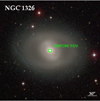 |
Fig. 1. Optical image of the galaxy NGC 1326. The field-of-view of our SINFONI observations is indicated. Image courtesy: Carnegie-Irvine Galaxy Survey (Ho et al. 2011). |
The presence of a low-ionization nuclear emission-line region (LINER) in the centre of this galaxy has been mentioned by Maia et al. (1987); however, as we mention in Sect. 3.1, no ionised gas is detected in the centre.
A particularly interesting nuclear star-forming ring with a mean radius r ≈ 300 pc is found at the ILR of the galaxy, visible in the Hubble Space Telescope (HST) composite image of the galaxy (Fig. 2). Garcia-Barreto et al. (1991) detected the ring in 20, 6, and 2 cm radio continuum emission and concluded that most of the emission is thermal.
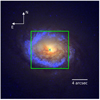 |
Fig. 2. Composite image from HST of the central region of NGC 1326 (red: F814W, green: F555W, blue: F336W). The box indicates the FOV of our SINFONI observations. The image was taken with the Wide Field and Planetary Camera 2 of the Hubble Space Telescope and retrieved from the Hubble Legacy Archive (http://hla.stsci.edu). Observations took place in January 1999 (proposal ID 6496, PI: R. Buta). |
The B − I colour index maps reveal that the ring is very blue and that there are complex dust patterns in the bar. Crocker et al. (1996) found that the inner ring is emitting 83% of the Hα luminosity. Buta et al. (2000) detected an asymmetric Hα emission in the ring with less emission on the west side, which Combes et al. (2019) do not see from CO(3–2) emission and thereby conclude that it is an extinction effect. Also the Buta et al. (2000) analysis of two-colour plots revealed that about 80% of the stellar clusters in the ring are < 50 Myr in age. Velocity fields suggest that the nuclear ring lies near the turn-over radius of the rotation curves (Storchi-Bergmann et al. 1996; Buta et al. 1998). The CO and Hα emission suggest the orientation of the ring to be roughly PA ∼ 90°, which is roughly perpendicular to the primary bar of the galaxy with PA ∼ 30° (Garcia-Barreto et al. 1991). Therefore Combes et al. (2019) indicate that the gas is either in x2 orbits or the nuclear ring is decoupled and has a higher pattern speed compared to the bar. Inside the nuclear ring Buta & Crocker (1993) detected strong dust lanes. The presence of a nuclear bar with position angle PA ∼ 90° (see Fig. 3) within the ring is discussed in, for example Erwin (2004), Laurikainen et al. (2006, 2011). However, these studies are only based on photometry (see a discussion on the kinematics in Sect. 3.8).
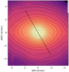 |
Fig. 3. K-band continuum extracted from the SINFONI data cube, by taking the median of the spectrum around λ ∼ 2.15 μm. The dashed line indicates the orientation of the large-scale bar (PA ∼ 30°, from Garcia-Barreto et al. 1991). The elongated isophote shape is due to the inclination of i = 53° of the large-scale disk of the galaxy. |
Throughout this paper, we adopt a luminosity distance of DL = 14.9 Mpc which is the median value of the redshift-independent distances in NED (Steer et al. 2017). This corresponds to a scale of 72.2 pc arcsec−1.
This paper is structured as follows: in Sect. 2 we present the observation and data reduction. In Sect. 3 we explain our analysis methods, show the results of our study, discuss the results, and compare these results with the literature. In Sect. 4 we present a summary of the results and the conclusions we draw from our study.
2. Observations and data reduction
The galaxy NGC 1326 was observed on October 6, 2014 with the NIR IFS SINFONI at the Very Large Telescope (VLT; e.g. Eisenhauer et al. 2003; Bonnet et al. 2004). We used the 8″ × 8″ field of view (FOV) in seeing-limited mode with H + K-band and K-band gratings for our observations. Using a jitter pattern we minimised the effect of bad pixels and increased the FOV to 9″ × 9″. The K-band grating was chosen for its high spectral resolution of 4000 (∼75 km s−1). While the H + K-band grating has a lower spectral resolution of only 1500 (∼200 km s−1), it offers a big spectral coverage and covers the region between H and K band, including the strong Paα line at 1.86 μm which cannot be observed with comparable instruments such as NIFS at the GEMINI telescope. The integration times spent on the target are 1500 s and 3000 s and on the sky are 750 s and 1500 s, for H + K band and K band, respectively.
The observed data were corrected for some detector pattern features using the model developed by Smajić et al. (2014) and were reduced to single exposure cubes using the ESO pipeline. For alignment, final coaddition, and telluric correction, we used our own PYTHON and IDL routines.
The G2V star Hip026810 was observed in between the science target observations to correct the data for atmospheric telluric absorption and for flux calibration. Two object-sky pairs for each band were taken, with an integration time of 1 s each. The intrinsic spectral features of the spectrum of the standard star were eliminated using a high-resolution solar spectrum (Maiolino et al. 1996), which was convolved with a Gaussian to match the spectral resolution of SINFONI.
The full width at half maximum (FWHM) of the point-spread function (PSF) is  and was measured by fitting a two-dimensional Gaussian profile to the combined images of the standard star. More information on the specifics of the data reduction and calibration can be found in Fazeli et al. (2019).
3. Results and discussion
We resolve the central ∼700 pc of NGC 1326. In the data cube we identify many emission lines: the hydrogen recombination lines Paα, Brγ, and Brδ; several ro-vibrational molecular hydrogen lines (H2(1–0)S(3) λ1.96 μm, H2(1–0)S(2) λ2.03 μm, H2(1–0)S(1) λ2.122 μm, H2(1–0)S(0) λ2.22 μm and H2(2–1)S(1) λ2.248 μm); the forbidden iron-line [Fe II]λ1.644 μm; He I; and stellar absorption features. These lines trace the physical conditions of different phases of the inter interstellar medium (ISM). In the following we discuss their brightness distributions and origins.
3.1. Emission-line flux distribution
The line fluxes were modelled by fitting single Gaussian functions to the line profiles. The continuum was subtracted by fitting a linear function to the continuum emission in two spectral windows, left and right from the emission line. For all fits we used the Levenberg-Marquardt algorithm included in the PYTHON implementation of LMFIT (Markwardt 2009; Newville et al. 2014). The emission line maps are clipped to have uncertainties less than 40%.
The emission flux maps of Brγ, H2λ2.122 μm, [Fe II] 1.644 μm, and He I are shown in Fig. 4. In all the maps we denote the position of the nucleus, where the continuum emission around 2.2 μm peaks, with an N. A few examples of the emission line fits are presented in Fig. 5.
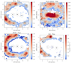 |
Fig. 4. Flux maps of the Brγλ2.166 μm, H2λ2.12 μm, [Fe II] λ1.644 μm, and He I emission lines. In all of the maps the flux units are 10−20 W m−2. The white pixels show the clipped regions with low S/N, where line fit uncertainties are above 40%. North is up and east is to the left. |
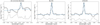 |
Fig. 5. Examples of the emission-line fits applied to apertures in the cubes (position of these apertures are illustrated in Fig. 4). |
3.1.1. Ionised gas
The most striking feature in all the line flux maps is strong emission from a circum-nuclear ring structure; however, there are differences in the emission peaks and strengths amongst the maps. Ionised gas, traced by the hydrogen recombination line Brγ, is only concentrated in the ring which has a radius of ∼4″ ≈ 300 pc. We do not detect emission within the ring and near the nucleus (central r ≈ 3″ region). With our data, we confirm the asymmetry of the ring reported by Buta et al. (2000) from the HST image of the Hα flux; our data is less affected by extinction than their optical data.
The patches on the east side show higher flux levels compared to the west side. Furthermore, there seem to be several gaps in the ring in the south and north-west. However we should stress that in our FOV we miss parts of the circum-nuclear ring in the east and west side.
The forbidden iron-transition [Fe II] 1.644 μm in the H band is slightly blended by the stellar absorption feature CO(7–4) at 1.641 μm. Therefore, prior to fitting this line, we used the PYTHON implementation of the penalized pixel-fitting method1 (PPXF; Cappellari & Emsellem 2004; Cappellari 2017) with default parameters to subtract the stellar absorption features. We employed a set of synthetic model spectra from Lançon et al. (2007), convolved with a Gaussian kernel to match the spectral resolution of our observation. We generate a spatially smoothed cube by applying a three-pixel boxcar filter to reach the necessary signal-to-noise ratio on the absorption features of the stellar continuum.
The flux distribution of [Fe II] looks very similar to that of Brγ, that is prominent in the circum-nuclear ring. However few differences are striking. While in the Brγ map the flux level varies amongst the patches, the emission of [Fe II] remains with similar strength on the east side of the ring. Also, on the west side of the ring the emission peaks of the patches are slightly shifted.
The emission from helium, which has an ionisation potential of ∼24.6 eV, is known as a tracer of regions with very hot and massive young stars. The flux distribution map of this line shows strong emissions in the north and south-east of the circum-nuclear ring. While the flux level of He I is lower than that of Brγ and therefore noisier, its distribution still resembles a very similar trend in the sense that ionised gas emission is much stronger in the east side of the ring, suggesting a higher excitation, possibly by star formation, on this side of the ring.
3.1.2. Molecular gas
The most prominent molecular hydrogen emission lines detected in the K band are H2(1–0)S(1) λ2.122 μm and H2(1–0)S(3) λ1.96 μm. We also detected H2(1–0)S(2) λ2.03 μm, H2(1–0)S(0) λ2.22 μm and H2(2–1)S(1) λ2.248 μm.
All these emission lines, tracing hot molecular gas, show similar flux distributions. We show the strongest line H2(1–0)S(1) in Fig. 4. The flux map shows a very different spatial distribution in comparison to Brγ. This line shows very strong flux levels in the centre. The emission is extended and reveals an elongated nuclear structure extended from east to west. In the circum-nuclear ring the emission of this gas is less prominent and less concentrated in comparison to Brγ and [Fe II].
3.2. Extinction
The dust reddening effect is significantly lower in the NIR compared to the optical, however it is not negligible. For a quantitative inspection of this effect, we present the extinction map (AV in mag) in Fig. 6, obtained from the H − K colour map. A derivation of the extinction map from emission line ratios was not feasible in this case owing to low and/or absent line emission in large portions of the FOV. The conversion of H − K values to AV are estimated using the following relation from Teixeira & Emerson (1999):
![Mathematical equation: $$ \begin{aligned} A_{ v} = k\,E(H-K) = k\,[(H-K)-(H-K)_0] . \end{aligned} $$](/articles/aa/full_html/2020/06/aa36451-19/aa36451-19-eq2.gif) (1)
(1)
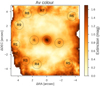 |
Fig. 6. Map of the extinction, derived from the H − K colour map. North is up and east is to the left. |
We employed the Calzetti et al. (2000) attenuation law for Galactic diffuse ISM (Rv = 3.12), which corresponds to a factor of k = 14.6 and an unreddened intrinsic colour of a typical quiescent galaxy of (H − K)0 = 0.22 (Glass 1984).
3.3. Emission line regions
The flux distribution maps show that there are several differences amongst the various regions in our FOV. Particularly the maps reveal structures in which ionised gas emits strongly in a circum-nuclear ring and molecular hydrogen emits strongly in an elongated nuclear structure.
To analyse the excitation properties in the nucleus (N), ring (R1 to R9), and within the ring (I1 and I2), we chose 11 apertures that are added to the maps in Fig. 4. We extracted spectra from these circular apertures with radii  . The spectra are shown in Fig. 7.
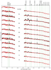 |
Fig. 7. Normalised spectra of the nuclear region and nine apertures in the circum-nuclear ring (R1-9) and two in the inside-the-ring regions (I1-2). The positions at which the apertures are extracted are indicated in Fig. 4. Several emission and absorption lines are indicated with green vertical lines. The stellar continuum fit is shown in red. |
Before proceeding with fitting the gas emission lines in these spectra, we modelled the stellar continuum with the PPXF method (shown in Fig. 7 in red). We then subtracted these models from the original spectra and used the residuals for the emission line fits. The measured line fluxes together with their 1σ standard errors, which are derived from the covariance matrix, are presented in Tables 1 and 2. All the line fluxes are corrected for extinction (see Sect. 3.2).
Molecular hydrogen emission lines in the apertures in the circum-nuclear ring, nucleus, and inside the ring regions, and derived quantities of hot and cold molecular gas mass.
Emission line fluxes in the apertures in the circum-nuclear ring and derived quantities, visual extinction, ionised gas mass, and SFR.
3.3.1. Near-infrared diagnostic diagrams
Diagnostic diagrams apply emission line flux ratios to differentiate between dominating excitation mechanisms. At NIR wavelengths the H I recombination lines are known as star formation tracers, and [Fe II] and H2 are prone to be stronger in regions excited by shocks or X-ray emission (e.g. from supernova remnants, outflows, or AGN).
In our study we used the H2λ2.12 μm/Brγ and [Fe II]λ1.644 μm/Brγ line ratios to investigate the apertures in the circum-nuclear ring (Fig. 8). The central apertures near the nucleus are excluded since they show no sign of Brγ nor [Fe II] emissions. The diagram has been divided into young star-forming, older supernova-dominated and compact AGN-dominated regions using the previous studies from Riffel et al. (2013) and Colina et al. (2015). The line ratios from apertures along the ring fall into regions of pure ionisation radiation (young starbursts), pure supernova-driven shock excitation, and in between. These are typical line ratios for clusters in circum-nuclear star-forming rings (e.g. Falcón-Barroso et al. 2014; Riffel et al. 2016; Busch et al. 2017; Fazeli et al. 2019).
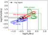 |
Fig. 8. Near-infrared diagnostic diagram with the line ratios log(H2λ2.12 μm/Brγ) vs. log([Fe II]λ1.644 μm/Brγ). The contours show the regions where young star formation, supernovae, and compact AGN are dominant and the solid lines denote the upper limits for young star-forming regions and AGN (from Colina et al. 2015). The dashed lines show the upper limits from another study by Riffel et al. (2013). |
We note that most of the spots in the circum-nuclear ring (R) are located in the young star formation regions. Particularly the apertures R2 and R7 show low ratios of [Fe II]/Brγ and also have high flux emissions in He I (Fig. 4), all of which are indications of young starburst regions. The apertures R1, R5, R6, and R8 lie in the supernova remnant-dominated region; however, very close to the lower limits. This means there are contributions from both shocks and photo-ionisation in these apertures and this hints at the fact that these parts of the ring have more intermediate-age stellar populations.
3.3.2. H2 excitation
The central kiloparsec of NGC 1326 is rich with a variety of H2 rotational vibrational transitions in the K band (Table 1). In general, molecular hydrogen can be excited by different mechanisms: (a) Thermal processes, in which shocks (Hollenbach & McKee 1989) induced by (e.g. radio jets) collisionally excite the gas or X-ray (Maloney et al. 1996) radiation from (e.g. the AGN) heats up the gas. (b) Non-thermal processes such as UV fluorescence mechanisms in which UV photons from (e.g. OB stars or strong AGN continuum) excite the H2 molecules (Black & van Dishoeck 1987).
In the H2 diagnostic diagram (Fig. 9) we indicate the regions in which each of the above-mentioned processes are the pure excitation source according to the models. However, in reality, the observed H2 spectra are produced by a mixture of these processes. But even so, the line ratio diagram can still be helpful in diagnosing which mechanism is the dominant excitation source.
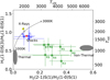 |
Fig. 9. Molecular hydrogen line ratio diagram of H2(1–0)S(3)/H2(1–0)S(1) vs. H2(2–1)S(1)/H2(1–0)S(1) (Mouri 1994; Rodríguez-Ardila et al. 2005). The grey curve shows the thermal emission at 1000−3000 K. The gray ellipse on the right represents the region in which models by Black & van Dishoeck (1987) predict non-thermal UV excitation. The grey ellipse on the left represents thermal UV excitation models by Sternberg & Dalgarno (1989). The yellow triangle represents the X-ray heating model by Draine & Woods (1990). The red star indicates the shock heating model by Brand et al. (1989). |
The line ratios of the analysed apertures are shown in Fig. 9. All the spots are located beneath the thermal Boltzmann distribution, meaning X-ray emission has less influence in exciting the molecular gas. We notice a clear gap between the apertures in the circum-nuclear ring (R1-9) and the apertures within the ring (I1-2, N). The central apertures have lower H2(2–1)S(1)/H2(1–0)S(1) ratios (0.08−0.12), which suggests that shocks are the thermal excitation mechanism that dominates in these regions. The patchy hot spots in the ring show higher H2(2–1)S(1)/H2(1–0)S(1) ratios (0.23−0.43) and are more inclined towards the non-thermal UV excitation mechanism. The latter ratios are similar to those in other circum-nuclear rings that show star formation activity (e.g. Falcón-Barroso et al. 2014; Riffel et al. 2016; Busch et al. 2017; Fazeli et al. 2019) and therefore strongly suggest star formation as the dominating H2 excitation mechanism. On the other hand, the behaviour for the other apertures is different, suggesting that these apertures are excited by a different mechanism and not by star formation. This is also consistent with the absence of hydrogen recombination lines in the centre, which would be expected in star formation regions.
The deficit Brγ emission in contrast to high H2 emission in the central 3″, especially in the nucleus aperture, suggests there is no AGN activity or recent star formation at the centre. Similar behaviour has been reported in other galaxies such as: NGC 4536, NGC 3351 and NGC 613 by Mazzalay et al. (2013) and Falcón-Barroso et al. (2014).
3.4. Star formation
One of the most striking structures in the central kiloparsec of NGC 1326 is the contrasted circum-nuclear ring. As revealed by the NIR diagnostic diagram (Fig. 8) the hotspots in the ring all show low H2/Brγ and [Fe II]/Brγ line ratios, indicate that the gas in these apertures is photo-ionised mainly by star formation. Also in the H2 excitation diagram (Fig. 9) the spots are more inclined towards the non-thermal excitation model, indicating a significant contribution of UV fluorescence to the gas excitation, which is consistent with star-forming regions. Furthermore, the stellar velocity dispersion (Fig. 10) shows lower values in the ring which is often associated to dynamically cold structures of young star-forming regions (see Sect. 3.6.1).
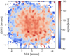 |
Fig. 10. Stellar velocity dispersion derived from a fit of stellar templates to the region around the CO(2–0) band head at a wavelength of ∼2.29 μm. White regions are clipped. North is up and east is to the left. |
3.4.1. Star formation rates
The luminosity of the hydrogen recombination lines is proportional to the Lyman continuum which is proportional to the recent star formation rate (SFR). In this section we use the luminosity of the Brγ emission line (Panuzzo et al. 2003) to estimate the SFR in different apertures as follows:
 (2)
(2)
In the apertures located in the star-forming ring the SFRs range from (4−17)×10−3 M⊙ yr−1. These measurements are listed in Table 2. The total Brγ emission flux, in the part of the ring that we observe in our FOV, is FBrγ = 1.2 × 10⁻¹⁴ erg s−1 cm−2, which leads to an SFR ≈ 0.2 M⊙ yr−1. Buta et al. (2000) estimated the SFR in the nuclear ring of NGC 1326 using the extinction corrected Hα line (FHα = 1.04 × 10⁻¹² erg s−1) and UV emission. For an area of 0.91 kpc2 these authors find SFR ≈ 1.1 M⊙ yr−1 kpc−2. For a better comparison we divide by the area that the ring covers in our FOV (≈0.26 kpc2) and get a star formation density of ≈0.8 M⊙ yr−1 kpc−2. These values are consistent, given uncertainties in the amount and patchiness of the extinction and in the assumed distances to the galaxy. We also look for the SFR per unit area in the apertures. They have a radius of  pc, which leads to 1−3 M⊙ yr−1 kpc−2. This value is at the lower end of typical SFR densities that are found on hundreds of parsec scales (1−50 M⊙ yr−1 kpc−1; Valencia-S. et al. 2012, and references therein).
3.4.2. Cluster ages
Finding the sequence in which the star formation proceeds in the ring can provide key information on the dynamics of the ILR. However, the existing methods to estimate cluster ages along the ring are very inaccurate.
Following the method from Böker et al. (2008) we approach this problem qualitatively. This method is far less affected by the underlying continuum emission from old stellar population in the disc and only compares the age of clusters qualitatively with each other and not the absolute age of the clusters. The method compares the fluxes of the emission lines He I, Brγ, and [Fe II] and thereby the different environments that lead to production of these emission lines. As mentioned in Sect. 3.3.1, Brγ and He I are photo-ionised in the Strömgren-spheres around O- and B-type stars. He I needs a higher ionisation energy and can therefore only be ionised by very massive stars that have a short lifetime of only a few million years. Therefore regions with younger clusters (few Myr) with hotter stars show higher He I/Brγ ratios. The assumptions are that the clusters have similar initial mass functions and are sufficiently massive that statistical variations in stellar inventory are insignificant. After around 10 Myr the supernova rate for an instantaneous burst reaches its maximum (see e.g. models of Leitherer et al. 1999). These supernovae create shocks that can produce partially ionised regions in which [Fe II] emission lines can be excited. This emission line is more dominant in clusters of ≳10 Myr in age.
In Fig. 11 we plot the flux of the [Fe II], Brγ, and He I emission lines for the nine ring apertures. It can be seen that in regions R1, R5, and R8 the emission line fluxes of Brγ and He I drop but for [Fe II] the emission line flux rises, which can mean that these regions are older compared to their neighbours. On the other hand in region R2 we see the opposite, meaning this region shows a younger starburst event. With this in mind, we cannot confirm a systematic gradient in cluster ages in the ring, as it is predicted for a “pearls-on-a-string” scenario in which starbursts happen through over-densities in particular spots in the ring and clusters then age while moving along this ring (Böker et al. 2008). Instead, the distribution of (relative) cluster ages looks rather stochastic.
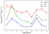 |
Fig. 11. Integrated flux of [Fe II] (red), Brγ (green), and He I (blue) emission lines in the circum-nuclear star-forming ring apertures. |
The apertures in the ring have Brγ equivalent widths in the range WBrγ = 3−10 Å. Comparing these values with the STARBURST99 (Leitherer et al. 2014, and the references therein) model predictions suggests ages of range 5−6 Myr (see e.g. Fig. 19 in Busch et al. 2017). However, owing to the contribution of underlying old stellar populations in the disc, the equivalent width is most probably underestimated, this means the estimated ages are an upper limit only. Buta et al. (2000) analysed the two-colour plots of the ring using HST data and suggested that the ring clusters have a wide range of ages. However, they reported that a significant population of the clusters are in age ranges of 1−10 Myr and more than 80% of the clusters have ages ≲50 Myr. These results are in agreement with our findings.
3.5. Gas masses
The extinction-corrected flux of the H2 1–0S(1) molecular hydrogen emission line can be used to estimate the mass of warm molecular gas (Scoville et al. 1982; Wolniewicz et al. 1998) as follows:
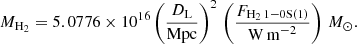 (3)
(3)
In this equation DL is the luminosity distance of the galaxy in Mpc and we assume that the gas is in local equilibrium and has a typical vibrational temperature of Tvib = 2000 K. As shown in the H2 excitation diagram (Fig. 9) this assumption is valid only for the central and inside the ring regions (I1-2), which however are the most significant contribution in our FOV. On the other hand, apertures in the ring show temperatures Tvib ≈ 3000−5000 K and we might overestimate the molecular gas mass by a factor of ∼2 in these regions (Busch et al. 2017). Even so, for better comparison with the literature values we follow the assumption.
The warm H2 (traced in NIR) is only emitted by the surface of a larger cold H2 gas reservoir. Studies show an empirical relation between the NIR warm H2 luminosities and the CO luminosities that trace the total molecular gas mass, suggesting the NIR H2 emission lines can be used to estimate the total molecular gas reservoir mass. We employ the conversion factor MH2(cold)/MH2(warm) = (0.3−1.6)×106 from Mazzalay et al. (2013).
We estimate the mass of ionised hydrogen gas using the extinction corrected flux of the hydrogen recombination line Brγ, FBrγ as follows:
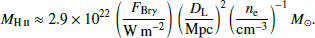 (4)
(4)
In this equation D is the distance to the galaxy in Mpc, assuming a temperature of T = 104 K, and an electron density of ne = 102 cm−3. We measure the gas masses in the apertures applying Eqs. (3) and (4); the values are listed in Tables 1 and 2.
We further estimate the gas masses by summing up the emission line fluxes (corrected for an average extinction of ∼1.5 mag) over the whole FOV. We find a total flux of FBrγ ≈ 1.2 × 10⁻¹⁷ W m−2, which leads to a gas mass of 8 × 10⁵ M⊙ for the ionised gas. Almost all of this gas is concentrated in the star formation ring, as shown in the flux map of Brγ emission line in Fig. 4.
For the molecular gas we measure the total flux to be 1.6 × 10⁻¹⁷ W m−2, which means there is a total warm molecular gas mass of 187 M⊙ in our FOV that corresponds to a cold gas mass of (0.6−3)×108 M⊙. Garcia-Barreto et al. (1991) reported a cold molecular H2 gas mass of 2.2 × 10⁸ M⊙ for an aperture of 44″ from CO emission observed with the SEST 15 m telescope.
In order to find the portion of the gas in the elongated structure in the centre and the ring we sum the H2 emission line flux in a central r = 3″ aperture, and in an annular aperture with a size of r = 3″ − 5″. Our measurements show warm molecular gas masses of 83 M⊙ in the elongated structure in the centre and 85 M⊙ in the ring, corresponding to cold gas masses of about ∼(0.2−1)×108 in each. In the CO(3–2) emission Combes et al. (2019, in their Fig. 2) detect the ring and the E–W structure although more clumpy, and they find a cold H2 mass of 1.3 × 10⁸ M⊙ in a 9″ × 9″ aperture, from which 52% is in the E–W structure and 48% is in the ring (F. Combes, priv. comm.). This is consistent with our results.
The AGNIFS group reported in Riffel et al. (2015), for nearby galaxies, warm molecular gas masses in the range 10 ≲ M(H2)≲103 M⊙ and ionised gas masses in the range 104 ≲ M(H II) ≲ 107 M⊙. Moser et al. (2012) using CO emission flux of nearby galaxies from the NUGA project, find cold molecular gas masses in the range 108 − 109 M⊙. We find the ratio of M(H II)/M(H2) ≈ 4300 in our FOV. As we show in Fazeli et al. (2019, and references therein) the ratio of ionised to warm molecular gas masses in nearby galaxies is in the range 2000−10 000 and for nearby QSOs this ratio is higher and can reach up to 20 000. The amounts of gas masses and ratios in NGC 1326 that we find therefore seem to be typical values observed in nearby galaxies.
3.6. Kinematics
3.6.1. Stellar kinematics
In this section, we analyse the motions of the stars in the central kiloparsec of NGC 1326. As a tracer for the stellar kinematics, we use the CO absorption lines in the K band, in particular the CO(2–0) absorption band head at a rest-frame wavelength of 2.29 μm.
The PPXF (Cappellari & Emsellem 2004; Cappellari 2017) is used with default parameters to fit stellar templates to the observed spectra in the spectral region from around 2.28 μm to 2.42 μm. We apply the Gemini library of late spectral templates (Winge et al. 2009), which contains NIR spectra of 29 late-type stars with spectral classes of F7 to M5 and was designed for velocity dispersion measurements like this. The stellar templates were convolved with a Gaussian kernel to match the spectral resolution of our observations. To reach the necessary signal to noise on the absorption features of the stellar continuum emission, we decided to smooth the data by applying a three-pixel boxcar filter.
In Fig. 10, we show a map of the fitted stellar velocity dispersion. We find a central velocity dispersion of about 110−120 km s−1, which is consistent with previous measurements, in particular the central velocity dispersion of (111 ± 14) km s−1 from HyperLeda2 (based on measurements by Dalle Ore et al. 1991). The velocity dispersion drops to values of ∼80 km s−1 where the star-forming ring is located. Star formation regions are known to show lower velocity dispersions, still resembling the dynamically cold gas reservoir from which they were formed (e.g. Riffel et al. 2011; Mazzalay et al. 2014; Busch et al. 2017).
In Fig. 12 (left), we show the stellar line-of-sight velocity (LOSV) map. White pixels were masked as a result of insufficient signal to noise on the absorption features. We find a clear rotation pattern with blue-shifted emission towards the north-east-east direction and red-shifted emission in the south-west-west. According to Buta et al. (2000) the south side is the near side of the galaxy. The velocity field appears very symmetric and has a maximum amplitude of about 100 km s−1 within the FOV.
 |
Fig. 12. Left: stellar LOSV map derived from fitting the spectral region around the CO(2–0) band head at ∼2.29 μm. Middle: model of the LOSV, assuming circular motions in a Plummer gravitational potential. Right: residuals after subtracting the model from the observed LOSV field. The systemic velocity derived in the model fit is subtracted from the maps. North is up and east is to the left. |
In order to quantify our findings, we fit a disc model to the radial velocity field. We assume that the stars follow Kepler orbits in the gravitational potential of the bulge which we describe with a Plummer function. The radial velocity field is then given by
![Mathematical equation: $$ \begin{aligned} { v}_{r} = { v}_{\rm s} + \sqrt{\frac{R^2 G M}{(R^2 + A^2)^{3/2}}} \frac{\sin (i) \cos (\Psi - \Psi _0)}{\left[\cos ^2(\Psi - \Psi _0) + \frac{\sin ^2(\Psi - \Psi _0)}{\cos ^2(i)}\right]^{3/4}}, \end{aligned} $$](/articles/aa/full_html/2020/06/aa36451-19/aa36451-19-eq8.gif) (5)
(5)
where vs is the systemic velocity of the disc, R and Ψ are cylindrical coordinates of each point in the projected plane of the sky, G is the gravitational constant, A is the scale length of the bulge, and M is the bulge mass (e.g. Barbosa et al. 2006; Smajić et al. 2015). The inclination i was fixed to 53° (from HyperLeda; Makarov et al. 2014) and the centre to the peak position of the continuum emission.
The resulting systemic velocity is (1399 ± 3) km s−1 (after heliocentric correction). For the PA of the line of nodes we find (74 ± 4)°, which is consistent with the photometric PA (75.6 ± 1.1)° (Laurikainen et al. 2006).
Storchi-Bergmann et al. (1996) analysed spectra from three long slits through the galaxy and fitted a rotating disc model to the data. These authors find a slightly lower systemic velocity of (1374 ± 11) km s−1. For the PA of the line of nodes, they find a value of (81 ± 3)°, which differs slightly from our results; this can be due to difference in the data and the FOV of the observations. However, since our new data set is based on an integral-field unit, we deem the new values to be more reliable.
In the middle panel of Fig. 12, we show a map of the model. The right panel shows the residuals after subtracting the model data from the observed LOSV map. Stochastic residuals with an amplitude of ≲20 km s−1 indicate a good match.
3.6.2. BH mass
To estimate the mass of the central SMBH, we fit the stellar velocity dispersion in a central aperture with radius r = 3″. This aperture size was chosen to exclude the nuclear star-forming ring.
Using PPXF with the same settings as described above, we derive a value of σ = (119 ± 5) km s−1, which is consistent with the former reported values in Hyperleda. We now apply the relation between BH mass MBH and stellar velocity dispersion σ of Kormendy & Ho (2013),
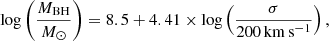 (6)
(6)
and find the mass of the BH to be log(MBH/M⊙) = 7.5. Because of the intrinsic scatter of the MBH − σ relations, we refrain from stating formal errors on the estimates. We conclude that the BH mass is of the order of a few 107 M⊙.
This is consistent with the value reported by Mutlu-Pakdil et al. (2016) of log(MBH/M⊙) = 7.47. These authors first fit a Spitzer 3.6 μm image, resulting in a Sersic-index of n = 2.21 and then applied the MBH − n relation of Graham & Driver (2007). A further consistent BH-mass estimate is reached, when we use the R-band bulge magnitude of mR = 11.2 that Gao & Ho (2017) derive from a detailed multi-component fit (taking into account bulge, disc, bar, and nuclear ring). We then apply the MBH − MR relation of Graham (2007) to get the BH mass of log(MBH/M⊙) = 7.6.
In contrast, Combes et al. (2019) find a significantly lower BH mass of log(MBH/M⊙) = 6.8, which they derive by modelling the gas velocities within the sphere of influence of the central BH. They argue that the deviation from previous estimates based on MBH − σ and MBH − Lbulge relations reflects the pseudo-bulge nature of this galaxy.
3.7. Gas velocity fields
In this section, we analyse the motion of molecular and ionised gas in the central kiloparsec of NGC 1326. Next to the emission line flux, the fit routine that was explained in Sect. 3.1 also delivers the central position and width of the emission lines for every spatial position. From the line centres, we derive the LOSV. Maps of the LOSV for Brγ, [Fe II], and H2(1–0)S(1) are shown in Fig. 13. White regions in the maps correspond to clipped areas, using the same criteria as for the emission line maps. The velocities are shown relative to the systemic velocity 1399 km s−1, as derived from the stellar velocity model (Sect. 3.6.1).
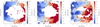 |
Fig. 13. Gas LOSVs for Brγ, [Fe II]λ1.644 μm, and H2(1–0)S(1)λ2.122 μm. The black cross in the centre indicate the continuum flux peak. The white pixels show the clipped regions with low S/N, where line fit uncertainties are above 40%. All velocities are given relative to the systemic velocity of 1399 km s−1. North is up and east is to the left. |
As already seen in the flux maps, emission of ionised (here Brγ) and partially ionised gas ([Fe II]) is only detected in the circum-nuclear ring. Therefore, we can only study the velocity field in the ring region. The velocity fields of all the emitting gas show rotation in the plane of the galaxy, red-shifted in the west and blue-shifted in the east, in accordance with the stellar kinematics, and a LOSV amplitude of 100 km s−1. The velocity field of [Fe II] seems slightly red-shifted with respect to the systemic velocity. However, the exact offset is difficult to estimate because of the lack of emission in the central region. The H2(1–0)S(1) line is detected in the centre, especially strong in a elongated nuclear structure spanning in east-west direction. While the overall velocity field follows a disc pattern similar to the stellar velocity field, velocities at the centre show deviations. We discuss this in further detail in the next section.
To cover the flux distribution of the H2 emission line at all velocities, including the asymmetric wings, we construct channel maps, shown in Fig. 14. Each panel shows the normalised emission line flux distribution integrated within velocity bins of 140 km s−1 (corresponding to two spectral pixels). We subtract the continuum emission by fitting a line to the spectra on the left and right side of the emission line. The centre of each velocity bin is shown on the top-right corner of the panels.
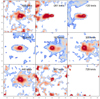 |
Fig. 14. Channel maps along the H2 emission line profile. Velocity bins are 140 km s−1 and centred on the velocities shown in the top left of the panels. The cross denotes the position of the nucleus. North is up and east is to the left. |
The channel maps reveal a spiral distribution from the north-east and east to the nuclear region, with blueshifts around −261 km s−1. At velocities about −120 km s−1 the flux distribution gets stronger on the east side of the nuclear elongated structure. At zero velocities the emission is mainly concentrated at the nucleus and in the 6″ elongated structure extending from the east to the west sides of the nucleus. As the velocities increase to positive values, at redshifts within 160 to 305 km s−1, the west side of the elongated nuclear structure appears stronger. In the centre, emission is present in almost all channels, indicating a high line width. This indicates a higher kinematical complexity, in particular compared to the star-forming ring region that shows rather confined lines.
3.8. Another bar-inside-a-bar or an inclined nuclear disc
Comparison of stellar and warm molecular gas kinematics (by subtracting the stellar velocity field from the gas velocity field) is a known method that can help find deviations of the gas motions from the regular motions in the stellar potential and reveal possible streaming motions in the central kiloparsec of galaxies. In many galaxies the rotation velocity of gas has a higher amplitude than that of the stars. This is because a significant part of the kinetic energy of the stars can go into random motion, while the molecular gas has lower velocity dispersion and is more confined to the galaxy plane.
When subtracting the stellar velocity field from the H2 velocity field of NGC 1326 (Fig. 15, left), it becomes apparent that we have to differentiate between two regions. In the star-forming ring, the residuals seem stochastic and of the order of ±20 km s−1. This indicates that the molecular gas in the ring follows the rotational motion in the stellar potential, similar to the ionised gas and the stellar velocity field. However within the ring, in the central 6″ elongated H2 structure, a clear deviation from the stellar velocity field is observed. On the one hand the velocity amplitudes appear higher than those in the ring region. On the other hand, the zero-velocity line in the H2 LOSV map (Fig. 13, right) appears to be twisted and has a shifted rotation PA in comparison to the star-forming ring and stellar velocity fields.
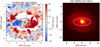 |
Fig. 15. Left: residuals after subtraction of the stellar velocity field from the molecular gas (H2(1–0)S(1)) velocity field. The black solid and dashed lines show the line of nodes and the zero-velocity line of the stellar LOSV model, respectively. The black box indicates the central 1″, where Combes et al. (2019) report a torus with a radius of 21 pc ∼ 0.3″ in the centre using the CO(3–2) emission. Right: map of HST F814W to compare the residual velocities with dust lanes, with which inflowing motions are often associated. North is up and east is to the left. |
This is in accordance with our previous findings that the star-forming ring and the central 6″ elongated H2 structure have different excitation mechanisms. While the gas is excited by UV photons from young star formation in the ring, the gas in the centre is thermally excited, most likely by shocks. The ring shows strong emission in ionised gas and the supernova-tracer [Fe II], which we associate with recent starbursts, while the centre shows none of those.
The most prominent feature inside the ring is the elongated H2 emission feature. Laurikainen et al. (2006, 2011) suggested that this feature, found in their H − K colour map, is a secondary bar inside the nuclear ring of NGC 1326. In this work, we use the advantage of having molecular H2 emission and CO absorption lines kinematics to look deeper into this elongated nuclear structure and try to understand its nature.
The stellar velocity field map and its residual from the model show no signs of perturbations, but rather a pure rotation in the plane of the galaxy (Fig. 12), this rules out the existence of a stellar bar. On the contrary, the residual map of the molecular gas and stellar LOSV (Fig. 15, left) reveals that the molecular gas in this structure has a much higher amplitude of the LOSV. One explanation for this deviation could be a higher inclination of the H2 structure in comparison to the disc of the galaxy. However the galaxy disc itself already has an inclination of i = 53° (Hyperleda inclination of the large-scale disc), which has a sin(i) = 0.8 (20% less than an edge-on disc rotation velocity). Therefore a simpler explanation would be that the stars (following the kinematics of the bulge) within the same radius as the elongated H2 structure do not rotate as fast, which is because most of their kinetic energy is going into random motion, which is evident in the stellar velocity dispersion map (Fig. 10). For an inclined object, it is difficult to say whether we see a nuclear bar or a gas disc.
Since the stellar LOSV map (Fig. 12) follows a pure rotation (no S-shaped or twisted zero-line velocity), we therefore suggest that there is no stellar bar. Bars that are purely gaseous, which means they occur without a stellar bar counterpart and are usually short-lived, therefore we suggest that the structure is more likely a central disc. The structure that Laurikainen et al. (2011) identified in the H − K colour map as a nuclear bar can be explained by the combination of the underlying continuum disc inclined with i = 53° (Hyperleda inclination of the large-scale disc) and the H2 emission which is elongated in E–W direction.
Going further to the centre, we see twisted zero-velocity lines that deviate in shape and angle from the zero-velocity lines of the stellar velocity field (compare Fig. 12 middle and Fig. 13 right). This can be interpreted as indication for another nuclear decoupled disc at the extremity of the gas structure in the central 1″. The position of this possible decoupled disc is indicated by a black box in the residual map (Fig. 15). While certainly higher resolution data is needed to investigate this feature in more detail, it is worth mentioning that this is the region for which Combes et al. (2019) report a torus with a radius of 21 pc ∼ 0.3″ in the centre using the CO(3–2) emission; this report would be consistent with our hypothesis.
In the case of NGC 1326, the amount of gas within the ring (in a central aperture of radius 3″) is about ∼(0.2−1)×108 M⊙; that is similar to the amount of gas found in the centre of some active galaxies (e.g. Mazzalay et al. 2013). In the optical continuum map (Fig. 15, right) there are dust lanes apparently connecting the elongated structure to the ring, This is indicated with a white ellipse. In many galaxies these dust features coincide with molecular gas streaming motions such as inflows (e.g. Davies et al. 2014; Busch et al. 2017; Fazeli et al. 2019).
We suspect the presence of other decoupled motions (Fig. 15, black box) from our kinematics maps, at the end of the nuclear disc (H2 extended structure). These decoupled structures can be drivers of gas inflows which provide fuel for the nucleus. However, currently there is no evidence for nuclear starburst or AGN activity in the centre. Combes et al. (2019) state that the torus in this galaxy is inclined on the sky plane in such a way that it could obscure the nucleus, leading to type 2 characteristics. Even in our NIR data, which is not as sensitive to extinction, we found no evidence of starburst or nuclear activity. This suggests that either NGC 1326 has no AGN at the centre or a “nascent” AGN is buried deeply in the dust, which can be a source of molecular hydrogen emission at the centre.
Storchi-Bergmann (2014) suggested that in LINERs gas is first accumulated in rings in the central few 100 pcs and then consumed by episodes of star formation, which are then followed by nuclear activity. This is in accordance with observations and simulations (e.g. Davies et al. 2007; Schawinski et al. 2009; Wild et al. 2010; Busch et al. 2015; Blank & Duschl 2016) that show a time delay between the onset of star formation in the central bulge and AGN activity of ∼100 Myr. Given that star formation and nuclear activity are considered to appear episodic, we might be observing the replenishment of molecular gas in the centre, which will lead to an episode of nuclear starburst and/or nuclear AGN activity in the centre in the future.
4. Summary and conclusions
We have analysed the NIR IFS data of the central kiloparsec of the galaxy NGC 1326 obtained with VLT- SINFONI and we found the following results:
-
We detect an elliptically shaped, circum-nuclear star-forming ring in our FOV. The ring is located at a radius of about 4″ ∼ 300 pc from the centre and contains patchy starburst regions with ages around ≲10 Myr. The starburst regions show stochastic age distributions along the ring.
-
Furthermore we detect ionised gas traced by Paα and Brγ as well as the supernova-tracer [Fe II] only in the circum-nuclear ring and not in the nuclear region, which means there is no sign of starburst or nuclear activity in the direct vicinity of the SMBH but only in the star-forming ring.
-
We estimate the BH mass, based on BH mass scaling relations to be MBH ≈ 3 × 10⁷ M⊙.
-
We find the warm molecular gas mass, using the H2 λ2.122 μm emission line flux, to be ∼187 M⊙, which corresponds to (0.6−3)×108 M⊙ of cold molecular gas mass. This value corresponds to the 9″ × 9″ FOV of the SINFONI data cube, from which half is concentrated in the star-forming ring and the other half in the central elongated feature extended from east to west side of the nucleus.
-
We also estimate the ionised gas mass, using flux of the hydrogen recombination emission line Brγ, to be ∼8 × 10⁵ M⊙. The ionised gas is mostly concentrated in the circum-nuclear ring and is absent in the central 3″. The ratio of ionised to molecular gas is around ≈4300 in the FOV, which is within the typical range observed in nearby galaxies.
-
The fits of CO band head absorption lines are used to study the stellar kinematics. The LOSV maps show a rotation in a disc in the plane of the galaxy, which is blue-shifted in the north-east and red-shifted in the west of the FOV.
-
Gas kinematics also show a rotation pattern with blueshift in the north-east and redshift in the south-west side, in agreement with the stellar kinematics. However, in the central r ≈ 3″ = 220 pc, the molecular gas shows higher amplitudes in the LOSV maps compared to the stellar velocity field. We suggest that since the stellar velocity fields show no sign of irregularities the H2 structure is not accompanied by a stellar bar component. We suggest that the H2 gas structure is probably a central disc within the ILR. The apertures in this structure are shock excited and the optical continuum map reveals dust lanes along this extended east to west 6″ H2 nuclear structure. The CO(3–2) emission observed with the Atacama Large Millimeter/submillimeter Array with higher resolution reveals a torus at the central
 nucleus region. In the velocity residual (H2−stellar losv) map of our SINFONI data, in the centre, we detect a hint of a further decoupled disc that has a slightly different PA from the elongated 6″ H2 structure as well. Higher resolution data are required to understand the complex kinematics at the centre of NGC 1326.
Near-infrared IFS allowed us to spatially resolve tracers of various gas phases and their kinematics with an unprecedented spatial resolution. With these means, we were able to resolve further features close to the nuclear centre on tens of parsec scales. It will be exciting to discover what new features next generation telescopes such as the Extremely Large Telescope will reveal on even smaller scales.
www-astro.physics.ox.ac.uk/∼mxc/software/PPXF version (V6.7.8).
Acknowledgments
The authors thank the anonymous referee for fruitful comments and suggestions. This research is carried out within the Collaborative Research Center 956, sub-project A2 (the studies of the conditions for star formation in nearby AGN and QSOs), funded by the Deutsche Forschungsgemeinschaft (DFG) – project ID 184018867. N. Fazeli is a member of the Bonn-Cologne Graduate School of Physics and Astronomy (BCGS).
References
- Barbosa, F. K. B., Storchi-Bergmann, T., Cid Fernandes, R., Winge, C., & Schmitt, H. 2006, MNRAS, 371, 170 [NASA ADS] [CrossRef] [Google Scholar]
- Bedregal, A. G., Colina, L., Alonso-Herrero, A., & Arribas, S. 2009, ApJ, 698, 1852 [NASA ADS] [CrossRef] [Google Scholar]
- Black, J. H., & van Dishoeck, E. F. 1987, ApJ, 322, 412 [NASA ADS] [CrossRef] [Google Scholar]
- Blank, M., & Duschl, W. J. 2016, MNRAS, 462, 2246 [CrossRef] [Google Scholar]
- Böker, T., Falcón-Barroso, J., Schinnerer, E., Knapen, J. H., & Ryder, S. 2008, AJ, 135, 479 [NASA ADS] [CrossRef] [Google Scholar]
- Bonnet, H., Abuter, R., Baker, A., et al. 2004, The Messenger, 117, 17 [NASA ADS] [Google Scholar]
- Brand, P. W. J. L., Toner, M. P., Geballe, T. R., et al. 1989, MNRAS, 236, 929 [NASA ADS] [CrossRef] [Google Scholar]
- Bureau, M., Mould, J. R., & Staveley-Smith, L. 1996, ApJ, 463, 60 [NASA ADS] [CrossRef] [Google Scholar]
- Busch, G., Smajić, S., Scharwächter, J., et al. 2015, A&A, 575, A128 [NASA ADS] [CrossRef] [EDP Sciences] [Google Scholar]
- Busch, G., Eckart, A., Valencia-S., M., et al. 2017, A&A, 598, A55 [NASA ADS] [CrossRef] [EDP Sciences] [Google Scholar]
- Buta, R., & Combes, F. 1996, Fund. Cosm. Phys., 17, 95 [Google Scholar]
- Buta, R., & Crocker, D. A. 1993, AJ, 105, 1344 [NASA ADS] [CrossRef] [Google Scholar]
- Buta, R., Alpert, A. J., Cobb, M. L., Crocker, D. A., & Purcell, G. B. 1998, AJ, 116, 1142 [NASA ADS] [CrossRef] [Google Scholar]
- Buta, R., Treuthardt, P. M., Byrd, G. G., & Crocker, D. A. 2000, AJ, 120, 1289 [NASA ADS] [CrossRef] [Google Scholar]
- Calzetti, D., Armus, L., Bohlin, R. C., et al. 2000, ApJ, 533, 682 [NASA ADS] [CrossRef] [Google Scholar]
- Cappellari, M. 2017, MNRAS, 466, 798 [NASA ADS] [CrossRef] [Google Scholar]
- Cappellari, M., & Emsellem, E. 2004, PASP, 116, 138 [NASA ADS] [CrossRef] [Google Scholar]
- Colina, L., Piqueras López, J., Arribas, S., et al. 2015, A&A, 578, A48 [NASA ADS] [CrossRef] [EDP Sciences] [Google Scholar]
- Combes, F., García-Burillo, S., Boone, F., et al. 2004, A&A, 414, 857 [NASA ADS] [CrossRef] [EDP Sciences] [Google Scholar]
- Combes, F., García-Burillo, S., Audibert, A., et al. 2019, A&A, 623, A79 [NASA ADS] [CrossRef] [EDP Sciences] [Google Scholar]
- Crocker, D. A., Baugus, P. D., & Buta, R. 1996, ApJS, 105, 353 [NASA ADS] [CrossRef] [Google Scholar]
- Dalle Ore, C., Faber, S. M., Jesus, J., Stoughton, R., & Burstein, D. 1991, ApJ, 366, 38 [NASA ADS] [CrossRef] [Google Scholar]
- Davies, R. I., Müller Sánchez, F., Genzel, R., et al. 2007, ApJ, 671, 1388 [NASA ADS] [CrossRef] [Google Scholar]
- Davies, R. I., Maciejewski, W., Hicks, E. K. S., et al. 2014, ApJ, 792, 101 [NASA ADS] [CrossRef] [Google Scholar]
- de Vaucouleurs, G. 1975, ApJS, 29, 193 [NASA ADS] [CrossRef] [Google Scholar]
- Draine, B. T., & Woods, D. T. 1990, ApJ, 363, 464 [NASA ADS] [CrossRef] [Google Scholar]
- Eisenhauer, F., Abuter, R., Bickert, K., et al. 2003, SPIE Conf. Ser., 4841, 1548 [Google Scholar]
- Erwin, P. 2004, A&A, 415, 941 [NASA ADS] [CrossRef] [EDP Sciences] [Google Scholar]
- Erwin, P. 2011, Mem. Soc. Astron. It. Suppl., 18, 145 [Google Scholar]
- Fabian, A. C. 2012, ARA&A, 50, 455 [NASA ADS] [CrossRef] [Google Scholar]
- Falcón-Barroso, J., Ramos Almeida, C., Böker, T., et al. 2014, MNRAS, 438, 329 [NASA ADS] [CrossRef] [Google Scholar]
- Fazeli, N., Busch, G., Valencia-S., M., et al. 2019, A&A, 622, A128 [NASA ADS] [CrossRef] [EDP Sciences] [Google Scholar]
- Gao, H., & Ho, L. C. 2017, ApJ, 845, 114 [NASA ADS] [CrossRef] [Google Scholar]
- Garcia-Barreto, J. A., Dettmar, R.-J., Combes, F., Gerin, M., & Koribalski, B. 1991, Rev. Mex. Astron. Astrofis., 22, 197 [Google Scholar]
- García-Burillo, S. 2016, IAU Symp., 315, 207 [Google Scholar]
- García-Burillo, S., & Combes, F. 2012, J. Phys. Conf. Ser., 372, 012050 [CrossRef] [Google Scholar]
- García-Burillo, S., Combes, F., Schinnerer, E., Boone, F., & Hunt, L. K. 2005, A&A, 441, 1011 [NASA ADS] [CrossRef] [EDP Sciences] [Google Scholar]
- Glass, I. S. 1984, MNRAS, 211, 461 [NASA ADS] [Google Scholar]
- Graham, A. W. 2007, MNRAS, 379, 711 [NASA ADS] [CrossRef] [Google Scholar]
- Graham, A. W., & Driver, S. P. 2007, ApJ, 655, 77 [NASA ADS] [CrossRef] [Google Scholar]
- Heckman, T. M., & Best, P. N. 2014, ARA&A, 52, 589 [Google Scholar]
- Hickox, R. C., Mullaney, J. R., Alexander, D. M., et al. 2014, ApJ, 782, 9 [NASA ADS] [CrossRef] [Google Scholar]
- Ho, L. C. 2008, ARA&A, 46, 475 [NASA ADS] [CrossRef] [Google Scholar]
- Ho, L. C., Li, Z.-Y., Barth, A. J., Seigar, M. S., & Peng, C. Y. 2011, ApJS, 197, 21 [NASA ADS] [CrossRef] [Google Scholar]
- Hollenbach, D., & McKee, C. F. 1989, ApJ, 342, 306 [NASA ADS] [CrossRef] [Google Scholar]
- Hopkins, P. F., & Quataert, E. 2010, MNRAS, 407, 1529 [NASA ADS] [CrossRef] [Google Scholar]
- Hopkins, P. F., Hernquist, L., Cox, T. J., & Kereš, D. 2008, ApJS, 175, 356 [NASA ADS] [CrossRef] [Google Scholar]
- Kim, W.-T., & Elmegreen, B. G. 2017, ApJ, 841, L4 [NASA ADS] [CrossRef] [Google Scholar]
- Kormendy, J. 1982, ApJ, 257, 75 [NASA ADS] [CrossRef] [Google Scholar]
- Kormendy, J., & Ho, L. C. 2013, ARA&A, 51, 511 [Google Scholar]
- Kormendy, J., Bender, R., & Cornell, M. E. 2011, Nature, 469, 374 [NASA ADS] [CrossRef] [Google Scholar]
- Lançon, A., Hauschildt, P. H., Ladjal, D., & Mouhcine, M. 2007, A&A, 468, 205 [NASA ADS] [CrossRef] [EDP Sciences] [Google Scholar]
- Laurikainen, E., Salo, H., Buta, R., et al. 2006, AJ, 132, 2634 [NASA ADS] [CrossRef] [Google Scholar]
- Laurikainen, E., Salo, H., Buta, R., & Knapen, J. H. 2011, MNRAS, 418, 1452 [NASA ADS] [CrossRef] [Google Scholar]
- Leitherer, C., Schaerer, D., Goldader, J. D., et al. 1999, ApJS, 123, 3 [NASA ADS] [CrossRef] [Google Scholar]
- Leitherer, C., Ekström, S., Meynet, G., et al. 2014, ApJS, 212, 14 [NASA ADS] [CrossRef] [Google Scholar]
- Maia, M. A. G., da Costa, L. N., Willmer, C., Pellegrini, P. S., & Rite, C. 1987, AJ, 93, 546 [NASA ADS] [CrossRef] [Google Scholar]
- Maiolino, R., Rieke, G. H., & Rieke, M. J. 1996, AJ, 111, 537 [NASA ADS] [CrossRef] [Google Scholar]
- Makarov, D., Prugniel, P., Terekhova, N., Courtois, H., & Vauglin, I. 2014, A&A, 570, A13 [CrossRef] [EDP Sciences] [Google Scholar]
- Maloney, P. R., Hollenbach, D. J., & Tielens, A. G. G. M. 1996, ApJ, 466, 561 [NASA ADS] [CrossRef] [Google Scholar]
- Markwardt, C. B. 2009, in Astronomical Data Analysis Software and Systems XVIII, eds. D. A. Bohlender, D. Durand, & P. Dowler, ASP Conf. Ser., 411, 251 [Google Scholar]
- Mazzalay, X., Saglia, R. P., Erwin, P., et al. 2013, MNRAS, 428, 2389 [NASA ADS] [CrossRef] [Google Scholar]
- Mazzalay, X., Maciejewski, W., Erwin, P., et al. 2014, MNRAS, 438, 2036 [NASA ADS] [CrossRef] [Google Scholar]
- Moser, L., Zuther, J., Busch, G., Valencia-S., M., & Eckart, A. 2012, Proceedings of Nuclei of Seyfert Galaxies and QSOs – Central Engine & Conditions of Star Formation (Seyfert 2012), 6–8 November, 2012, Max-Planck-Insitut für Radioastronomie (MPIfR), Bonn, Germany, Online at http://pos.sissa.it/cgi-bin/reader/conf.cgi?confid=169, 69 [Google Scholar]
- Mouri, H. 1994, ApJ, 427, 777 [NASA ADS] [CrossRef] [Google Scholar]
- Mutlu-Pakdil, B., Seigar, M. S., & Davis, B. L. 2016, ApJ, 830, 117 [NASA ADS] [CrossRef] [Google Scholar]
- Newville, M., Stensitzki, T., Allen, D. B., & Ingargiola, A. 2014, https://doi.org/10.5281/zenodo.11813 [Google Scholar]
- Panuzzo, P., Bressan, A., Granato, G. L., Silva, L., & Danese, L. 2003, A&A, 409, 99 [NASA ADS] [CrossRef] [EDP Sciences] [Google Scholar]
- Riffel, R., Riffel, R. A., Ferrari, F., & Storchi-Bergmann, T. 2011, MNRAS, 416, 493 [NASA ADS] [Google Scholar]
- Riffel, R. A., Storchi-Bergmann, T., & Winge, C. 2013, MNRAS, 430, 2249 [NASA ADS] [CrossRef] [Google Scholar]
- Riffel, R. A., Storchi-Bergmann, T., & Riffel, R. 2015, MNRAS, 451, 3587 [NASA ADS] [CrossRef] [Google Scholar]
- Riffel, R. A., Colina, L., Storchi-Bergmann, T., et al. 2016, MNRAS, 461, 4192 [NASA ADS] [CrossRef] [Google Scholar]
- Rodríguez-Ardila, A., Riffel, R., & Pastoriza, M. G. 2005, MNRAS, 364, 1041 [NASA ADS] [CrossRef] [Google Scholar]
- Sanders, D. B., Soifer, B. T., Elias, J. H., et al. 1988, ApJ, 325, 74 [NASA ADS] [CrossRef] [Google Scholar]
- Schawinski, K., Virani, S., Simmons, B., et al. 2009, ApJ, 692, L19 [NASA ADS] [CrossRef] [Google Scholar]
- Schawinski, K., Koss, M., Berney, S., & Sartori, L. F. 2015, MNRAS, 451, 2517 [NASA ADS] [CrossRef] [Google Scholar]
- Scoville, N. Z., Hall, D. N. B., Ridgway, S. T., & Kleinmann, S. G. 1982, ApJ, 253, 136 [NASA ADS] [CrossRef] [Google Scholar]
- Shlosman, I., Frank, J., & Begelman, M. C. 1989, Nature, 338, 45 [NASA ADS] [CrossRef] [Google Scholar]
- Smajić, S., Fischer, S., Zuther, J., & Eckart, A. 2012, A&A, 544, A105 [NASA ADS] [CrossRef] [EDP Sciences] [Google Scholar]
- Smajić, S., Moser, L., Eckart, A., et al. 2014, A&A, 567, A119 [NASA ADS] [CrossRef] [EDP Sciences] [Google Scholar]
- Smajić, S., Moser, L., Eckart, A., et al. 2015, A&A, 583, A104 [NASA ADS] [CrossRef] [EDP Sciences] [Google Scholar]
- Steer, I., Madore, B. F., Mazzarella, J. M., et al. 2017, AJ, 153, 37 [NASA ADS] [CrossRef] [Google Scholar]
- Sternberg, A., & Dalgarno, A. 1989, ApJ, 338, 197 [NASA ADS] [CrossRef] [Google Scholar]
- Storchi-Bergmann, T. 2014, IAU Symp., 303, 354 [Google Scholar]
- Storchi-Bergmann, T., Rodriguez-Ardila, A., Schmitt, H. R., Wilson, A. S., & Baldwin, J. A. 1996, ApJ, 472, 83 [NASA ADS] [CrossRef] [Google Scholar]
- Storchi-Bergmann, T., & Schnorr-Müller, A. 2019, Nat. Astron., 3, 48 [NASA ADS] [CrossRef] [Google Scholar]
- Teixeira, T. C., & Emerson, J. P. 1999, A&A, 351, 303 [NASA ADS] [Google Scholar]
- Treister, E., Schawinski, K., Urry, C. M., & Simmons, B. D. 2012, ApJ, 758, L39 [NASA ADS] [CrossRef] [Google Scholar]
- Valencia-S., M., Zuther, J., Eckart, A., et al. 2012, A&A, 544, A129 [NASA ADS] [CrossRef] [EDP Sciences] [Google Scholar]
- Valencia-S., M., Busch, G., & Smajić, S. 2014, IAU Symp., 304, 274 [Google Scholar]
- Wild, V., Heckman, T., & Charlot, S. 2010, MNRAS, 405, 933 [NASA ADS] [Google Scholar]
- Winge, C., Riffel, R. A., & Storchi-Bergmann, T. 2009, ApJS, 185, 186 [NASA ADS] [CrossRef] [Google Scholar]
- Wolniewicz, L., Simbotin, I., & Dalgarno, A. 1998, ApJS, 115, 293 [NASA ADS] [CrossRef] [Google Scholar]
- Zuther, J., Iserlohe, C., Pott, J. U., et al. 2007, A&A, 466, 451 [NASA ADS] [CrossRef] [EDP Sciences] [Google Scholar]
All Tables
Molecular hydrogen emission lines in the apertures in the circum-nuclear ring, nucleus, and inside the ring regions, and derived quantities of hot and cold molecular gas mass.
Emission line fluxes in the apertures in the circum-nuclear ring and derived quantities, visual extinction, ionised gas mass, and SFR.
All Figures
|
Fig. 1. Optical image of the galaxy NGC 1326. The field-of-view of our SINFONI observations is indicated. Image courtesy: Carnegie-Irvine Galaxy Survey (Ho et al. 2011). |
| In the text | |
|
Fig. 2. Composite image from HST of the central region of NGC 1326 (red: F814W, green: F555W, blue: F336W). The box indicates the FOV of our SINFONI observations. The image was taken with the Wide Field and Planetary Camera 2 of the Hubble Space Telescope and retrieved from the Hubble Legacy Archive (http://hla.stsci.edu). Observations took place in January 1999 (proposal ID 6496, PI: R. Buta). |
| In the text | |
|
Fig. 3. K-band continuum extracted from the SINFONI data cube, by taking the median of the spectrum around λ ∼ 2.15 μm. The dashed line indicates the orientation of the large-scale bar (PA ∼ 30°, from Garcia-Barreto et al. 1991). The elongated isophote shape is due to the inclination of i = 53° of the large-scale disk of the galaxy. |
| In the text | |
|
Fig. 4. Flux maps of the Brγλ2.166 μm, H2λ2.12 μm, [Fe II] λ1.644 μm, and He I emission lines. In all of the maps the flux units are 10−20 W m−2. The white pixels show the clipped regions with low S/N, where line fit uncertainties are above 40%. North is up and east is to the left. |
| In the text | |
|
Fig. 5. Examples of the emission-line fits applied to apertures in the cubes (position of these apertures are illustrated in Fig. 4). |
| In the text | |
|
Fig. 6. Map of the extinction, derived from the H − K colour map. North is up and east is to the left. |
| In the text | |
|
Fig. 7. Normalised spectra of the nuclear region and nine apertures in the circum-nuclear ring (R1-9) and two in the inside-the-ring regions (I1-2). The positions at which the apertures are extracted are indicated in Fig. 4. Several emission and absorption lines are indicated with green vertical lines. The stellar continuum fit is shown in red. |
| In the text | |
|
Fig. 8. Near-infrared diagnostic diagram with the line ratios log(H2λ2.12 μm/Brγ) vs. log([Fe II]λ1.644 μm/Brγ). The contours show the regions where young star formation, supernovae, and compact AGN are dominant and the solid lines denote the upper limits for young star-forming regions and AGN (from Colina et al. 2015). The dashed lines show the upper limits from another study by Riffel et al. (2013). |
| In the text | |
|
Fig. 9. Molecular hydrogen line ratio diagram of H2(1–0)S(3)/H2(1–0)S(1) vs. H2(2–1)S(1)/H2(1–0)S(1) (Mouri 1994; Rodríguez-Ardila et al. 2005). The grey curve shows the thermal emission at 1000−3000 K. The gray ellipse on the right represents the region in which models by Black & van Dishoeck (1987) predict non-thermal UV excitation. The grey ellipse on the left represents thermal UV excitation models by Sternberg & Dalgarno (1989). The yellow triangle represents the X-ray heating model by Draine & Woods (1990). The red star indicates the shock heating model by Brand et al. (1989). |
| In the text | |
|
Fig. 10. Stellar velocity dispersion derived from a fit of stellar templates to the region around the CO(2–0) band head at a wavelength of ∼2.29 μm. White regions are clipped. North is up and east is to the left. |
| In the text | |
|
Fig. 11. Integrated flux of [Fe II] (red), Brγ (green), and He I (blue) emission lines in the circum-nuclear star-forming ring apertures. |
| In the text | |
|
Fig. 12. Left: stellar LOSV map derived from fitting the spectral region around the CO(2–0) band head at ∼2.29 μm. Middle: model of the LOSV, assuming circular motions in a Plummer gravitational potential. Right: residuals after subtracting the model from the observed LOSV field. The systemic velocity derived in the model fit is subtracted from the maps. North is up and east is to the left. |
| In the text | |
|
Fig. 13. Gas LOSVs for Brγ, [Fe II]λ1.644 μm, and H2(1–0)S(1)λ2.122 μm. The black cross in the centre indicate the continuum flux peak. The white pixels show the clipped regions with low S/N, where line fit uncertainties are above 40%. All velocities are given relative to the systemic velocity of 1399 km s−1. North is up and east is to the left. |
| In the text | |
|
Fig. 14. Channel maps along the H2 emission line profile. Velocity bins are 140 km s−1 and centred on the velocities shown in the top left of the panels. The cross denotes the position of the nucleus. North is up and east is to the left. |
| In the text | |
|
Fig. 15. Left: residuals after subtraction of the stellar velocity field from the molecular gas (H2(1–0)S(1)) velocity field. The black solid and dashed lines show the line of nodes and the zero-velocity line of the stellar LOSV model, respectively. The black box indicates the central 1″, where Combes et al. (2019) report a torus with a radius of 21 pc ∼ 0.3″ in the centre using the CO(3–2) emission. Right: map of HST F814W to compare the residual velocities with dust lanes, with which inflowing motions are often associated. North is up and east is to the left. |
| In the text | |
Current usage metrics show cumulative count of Article Views (full-text article views including HTML views, PDF and ePub downloads, according to the available data) and Abstracts Views on Vision4Press platform.
Data correspond to usage on the plateform after 2015. The current usage metrics is available 48-96 hours after online publication and is updated daily on week days.
Initial download of the metrics may take a while.