| Issue |
A&A
Volume 637, May 2020
|
|
|---|---|---|
| Article Number | A60 | |
| Number of page(s) | 20 | |
| Section | Stellar structure and evolution | |
| DOI | https://doi.org/10.1051/0004-6361/202037452 | |
| Published online | 14 May 2020 | |
The mass discrepancy in intermediate- and high-mass eclipsing binaries: The need for higher convective core masses
1
Institute of Astronomy, KU Leuven, Celestijnenlaan 200D, 3001 Leuven, Belgium
e-mail: This email address is being protected from spambots. You need JavaScript enabled to view it.
2
Department of Physics, Faculty of Science, University of Zagreb, Bijenicka Cesta 32, 10000 Zagreb, Croatia
3
Astrophysics Group, Keele University, Staffordshire ST5 5BG, UK
4
Institute of Astronomy, Russian Academy of Sciences, Pyatnitskaya Str., 48, Moscow 119017, Russia
5
Department of Astrophysics/IMAPP, Radboud University Nijmegen, 6500 GL Nijmegen, The Netherlands
6
Max Planck Institute for Astronomy, Koenigstuhl 17, 69117 Heidelberg, Germany
Received:
7
January
2020
Accepted:
19
March
2020
Abstract
Context. Eclipsing, spectroscopic double-lined binary star systems are excellent laboratories for calibrating theories of stellar interior structure and evolution. Their precise and accurate masses and radii measured from binary dynamics offer model-independent constraints and challenge current theories of stellar evolution.
Aims. We aim to investigate the mass discrepancy in binary stars. This is the significant difference between stellar components’ masses measured from binary dynamics and those inferred from models of stellar evolution via positions of the components in the Teff − log g Kiel diagram. We study the effect of near-core mixing on the mass of the convective core of the stars and interpret the results in the context of the mass discrepancy.
Methods. We fitted stellar isochrones computed from a grid of MESA stellar evolution models to a homogeneous sample of eleven high-mass binary systems. Two scenarios are considered where individual stellar components of a binary system are treated independent of each other and where they are forced to have the same age and initial chemical composition. We also study the effect of the microturbulent velocity and turbulent pressure on the atmosphere model structure and stellar spectral lines, and its link with the mass discrepancy.
Results. We find that the mass discrepancy is present in our sample and that it is anti-correlated with the surface gravity of the star. No correlations are found with other fundamental and atmospheric parameters, including the stellar mass. The mass discrepancy can be partially accounted for by increasing the amount of near-core mixing in stellar evolution models. We also find that ignoring the microturbulent velocity and turbulent pressure in stellar atmosphere models of hot evolved stars results in the overestimation of their effective temperature by up to 8%. Together with enhanced near-core mixing, this can almost entirely account for the ∼30% mass discrepancy found for the evolved primary component of V380 Cyg.
Conclusions. We find a strong link between the mass discrepancy and the convective core mass. The mass discrepancy can be solved by considering the combined effect of extra near-core boundary mixing and the consistent treatment in the spectrum analysis of hot evolved stars. Our binary modelling results in convective core masses between 17 and 35% of the stellar mass, which is in excellent agreement with the results from gravity-mode asteroseismology of single stars. This implies larger helium core masses near the end of the main sequence than have been anticipated so far.
Key words: methods: data analysis / methods: numerical / techniques: spectroscopic / binaries: eclipsing / binaries: spectroscopic / stars: general
© ESO 2020
1. Introduction
The theory of stellar interior structure and evolution (SSE) plays a crucial role in contemporary astrophysics. Many research fields rely on predictions of this theory and are hence extremely dependent on how well physical conditions can be described throughout the star, both instantaneously and as a function of time. Historically, the theory of SSE was calibrated on surface atmospheric properties of stars, meaning that the whole process was largely driven by observational constraints that were only available at the outer (atmospheric) boundary. The situation significantly improved in the case of the Sun with the advent of helioseismology (e.g. Leighton et al. 1962; Evans & Michard 1962a,b,c; Christensen-Dalsgaard & Gough 1976; Harvey et al. 1996; Gough et al. 1996; Christensen-Dalsgaard 2002), which allowed more than 70% of the outermost part of the Sun to be probed through the detection and interpretation of its acoustic waves stochastically driven by convection (Claverie et al. 1979; Duvall & Harvey 1983).
Helioseismology has provided an enormous improvement in the calibration of the models for low-mass stars with a radiative core (Christensen-Dalsgaard 2002). This was achieved from adapting the input physics and parametrised transport profiles in models of the Sun to solve discrepancies in the solar oscillation frequencies and those predicted by non-rotating non-magnetic 1D models. This seismically calibrated solar model is nowadays applied to the thousands of low-mass and evolved intermediate-mass stars observed with the Kepler (Borucki et al. 2010) and TESS (Ricker et al. 2015) space missions. The frequencies of their pressure (p-) modes allow us to determine the radii, masses and and ages of solar-like stars from scaling them with respect to the frequencies of the helioseismic solar model, leading to relative precisions for the stellar radii, masses, and ages of ∼2, ∼5, and ∼15%, respectively (Chaplin et al. 2014; Hekker & Christensen-Dalsgaard 2017). Higher precisions require improving the input physics, starting from the non-rotating non-magnetic solar-scaled model and adopting its ingredients to include more realistic descriptions for the transport processes due to convection, atomic diffusion, rotation, and magnetism so as to meet the asteroseismic measurements (e.g. Silva Aguirre et al. 2017; Verma & Silva Aguirre 2019; Eggenberger et al. 2019a,b; Fuller et al. 2019).
Asteroseismic evaluations of intermediate- and high-mass stars in the core-hydrogen burning phase are based on a similar principle to helio- and asteroseismology of low-mass stars. However, evaluations of intermediate- and high-mass stars cannot rely on the scaling of solar-like models, since they have a convective core and a radiative envelope. For an extensive discussion of the methodology and a summary of achievements so far, we refer to Aerts (2019). For the current work, we distill the two most pertinent results obtained from some 40 intermediate-mass stars covering M ∈ [1.3, 8] M⊙ deduced from non-radial gravity (g) modes, which probe the region just outside the convective core: (1) stars with a convective core are near-rigid rotators throughout the entire core-hydrogen burning phase across the modelled range of veq/vcrit ∈ [0, 70]% (Aerts et al. 2019); (2) asteroseismic derivations of the mass of the convective core, Mcc, via the estimation of near-core mixing levels, lead to the broad range of Mcc/M ∈ [3, 20]%. These studies pinpoint the need for more massive convective cores during the main-sequence phase compared with those predicted by standard stellar evolution models, even when limiting to the slowest rotators in the sample.
Much in the spirit of helioseismology, the asteroseismic studies of intermediate- and high-mass stars purposefully do not specify the physical reason for the extra mixing near the convective core but rather interpret the deviations between g-mode frequencies predicted for 1D non-rotating non-magnetic stellar models and those detected in the space-based data. It is noteworthy to mention that the mixing profiles predicted from various 1D rotating stellar models differ by a lot, but they also do not lead to appropriate values of g-mode frequencies when compared with space asteroseismic data of such quantities (Aerts et al. 2018). In particular, the predicted levels of chemical mixing at the bottom of the deep envelopes of the models due to rotational instabilities are orders of magnitude too high to be in agreement with the asteroseismic data.
Eclipsing doubled-lined spectroscopic binaries offer a completely independent way to calibrate the interiors of intermediate- and high-mass stars. The ability to infer model-independent masses and radii of stars with very high precision and accuracy makes binary stars ideal candidates for benchmarking SSE models as well as asteroseismic analyses. Valle et al. (2018) performed a theoretical study as to the ability to recover stellar ages and the overshooting efficiency based on simulated binary star data. The authors assumed typical observational uncertainties on stellar mass and effective temperature of ≤1% and ±150 K, respectively. Moreover, they also found that recovered ages and efficiencies of near core mixing are biased towards lower values in all considered scenarios. Valle et al. (2018) also concluded that the above observational uncertainties typically allow one to distinguish between models without convective core overshooting and those with an intermediate amount of convective core overshooting.
Pols et al. (1997) already showed that SSE models require systematically enhanced near-core mixing at post-main-sequence stage of evolution to accommodate stellar masses measured from binary dynamics. Lastennet & Valls-Gabaud (2002) report an overall agreement between model predictions and mass and radius measurements for 60 detached binary systems, emphasizing a large degeneracy between the age and metallicity in the models due to lack of observational constraints for the metallicity. More recently, Higl & Weiss (2017) presented a study of detached eclipsing binaries in a wide range of stellar masses. These authors report the need to introduce extra near-core mixing in the form of overshooting for stars with a convective core.
Binary and multiple stellar systems are also found to be extremely synergistic with intrinsically variable pulsating stars. An example of such a synergy is the class of “heart-beat stars” (Thompson et al. 2012) – highly eccentric binaries with variable component(s), where the pulsational variability is being triggered by tidal forces (e.g. Welsh et al. 2011; Hambleton et al. 2013a,b; Guo et al. 2019). In addition to providing a stellar pulsation excitation mechanism, tides are also known to be important (Fuller 2017; Guo et al. 2017) and can affect self-excited oscillations of stars, as evidenced recently by the TESS mission (e.g. Bowman et al. 2019).
2. The mass discrepancy
The SSE models of stars born with a convective core are not well calibrated. A striking example is the mass discrepancy observed in massive stars which has remained unsolved for almost three decades. The original formulation of the problem comes from Herrero et al. (1992), who presented a spectroscopic analysis of 25 luminous Galactic stars and made a comparison between spectroscopically inferred masses and those derived from models of stellar evolution. The spectroscopic masses are derived by exploiting the spectroscopically determined surface gravities and radii that come from the absolute visual magnitude MV of the star and the integral of stellar flux V (Eq. (1) in Herrero et al. 1992). The evolutionary masses are in turn obtained by fitting evolutionary tracks to the position of the star in the Hertzsprung-Russell (HR) diagram, where stellar luminosity is derived from the radius and the spectroscopically inferred effective temperature of the star. From a comparison of the component masses within the sample, the authors concluded that SSE models overpredict the masses of the stars and that there is a tendency of the effect to get more pronounced as the surface gravity log g of the star decreases (see Fig. 16 in Herrero et al. 1992).
The conclusions of Herrero et al. (1992) are confirmed by independent studies of eclipsing, spectroscopic double-lined (SB2) binaries. In this particular case, it is the dynamical versus evolutionary mass discrepancy that is being reported. While the former mass measurement is model-independent and comes from binary dynamics, the latter mass inference is based on fitting positions of individual stellar components in the HR diagram with evolutionary tracks.
2.1. Case study: V380 Cyg
The binary V380 Cyg comprises an evolved early B-type primary star and a main-sequence B-type secondary. It is amongst the most prominent cases of massive binaries exhibiting the mass discrepancy. The system was originally studied by Guinan et al. (2000) based on time-series of multi-color ground-based photometric data and of high-resolution optical échelle spectroscopy. The authors emphasised the difficulty to explain the position of the more evolved primary in the HR diagram with evolutionary tracks that correspond to the dynamical mass, spectroscopically measured metallicity, and no extra mixing in the near-core regions of the primary. Large amounts of extra near-core mixing in the form of convective penetration corresponding to αov = 0.6 was proposed by Guinan et al. (2000) as a possible solution to the mass discrepancy in the V380 Cyg system. The need for a large amount of extra mixing in the near-core region has been confirmed quasi-independently by the authors from measurements of the apsidal motion of the star and subsequent inference of the internal structure constant k.
The system was revisited by Pavlovski et al. (2009) based on photometric data of Guinan et al. (2000) and newly obtained multi-instrument extended time-series of optical échelle high-resolution spectroscopy. The authors used the method of spectral disentangling (SPD; Simon & Sturm 1994) as implemented in the FDBINARY software package (Ilijic et al. 2004) to disentangle composite spectra of the binary system into individual spectral contributions of the two components. Atmospheric characteristics inferred from the disentangled spectra were used with a grid of Geneva evolutionary models to derive evolutionary masses of the two stars. In line with the findings by Guinan et al. (2000), the authors report a mass discrepancy in excess of 10% for the more evolved primary component, by comparing its dynamical mass to a set of evolutionary masses inferred from the SSE model grids of Schaller et al. (1992), Claret (1995), and Ekström et al. (2008). In particular, Pavlovski et al. (2009) conclude that the current numerical implementation of rotation in SSE models does not solve the mass discrepancy observed in V380 Cyg.
V380 Cyg was one of the brightest and most massive stars observed by the Kepler space mission in its Guest Observer Programme (PI: A. Tkachenko). Hence, it was reanalysed once again by Tkachenko et al. (2014) based on about three months of nearly continuous Kepler space photometry and newly obtained time-series of optical échelle spectroscopy from the HERMES spectrograph mounted on the Flemish Mercator telescope on La Palma (Raskin et al. 2011). Similar to the previous studies, the authors report a mass discrepancy in excess of 30% for the primary component. The measurements could only be explained by assuming a stellar mass at 3σ of its dynamical value, by significantly increasing the initial rotation rate compared to the current one, and by adopting a high value of αov = 0.6 in their grid of MESA evolutionary models computed according to Paxton et al. (2013). In addition, Tkachenko et al. (2014) also report the detection of stochastic oscillations intrinsic to the primary component, as well as rotational modulation in the high-resolution spectroscopy.
2.2. Ensemble study results
Schneider et al. (2014) presented a homogeneous Bayesian analysis of a sample of 18 eclipsing binaries from the Torres et al. (2010) sample and relied on Bonn stellar evolution models with rotation. The authors stressed that rotation implies a larger radius of a few percent and hence can not be ignored. Furthermore, Schneider et al. (2014) focused on the consequences of rotational mixing in stellar ageing, while assuming that stars with fractional main-sequence ages less than 35% are unaffected by convective core overshooting. Under these conditions, they were able to find a good isochrone fit for component stars cooler than 25 000 K. Here, we take a similar approach but lift the assumption that stars do not experience near-core mixing in the first stage of the main sequence, since asteroseismology has shown young massive stars experience near-core boundary mixing (see Aerts 2019, for a summary of measured near-core and envelope mixing levels). Moreover, we consider models with near-core mixing without specifying its origin in terms of physical process, again following recent results from asteroseismology. We evaluate the models for a sample of eclipsing binaries with high-resolution spectroscopy analysed in a homogeneous way so as to eliminate systematic bias in the data that is used as input for the modelling. In this respect, our study can be seen as a follow-up study of the one by Schneider et al. (2014), but where we utilize non-rotating models with interior mixing prescriptions guided by asteroseismology.
The idea of probing the amount of near-core mixing in intermediate- and high-mass binaries in the form of convective core overshooting has been further elaborated upon by Claret & Torres (2016, 2017, 2018, 2019) in their series of papers on a sample of some 50 eclipsing SB2 systems. Their sample has been compiled from the catalogue of Torres et al. (2010) and the catalogue of the Optical Gravitational Microlensing Experiment (OGLE)1. The selection requirements concerned precise and accurate (3% and better) masses, radii, and effective temperatures of stars, with additional selection criteria being evolutionary stage and availability of the surface chemical composition measurements. Grids of non-rotating evolutionary models were computed with the Granada (Claret 2004, 2012) and MESA (Paxton et al. 2011, 2013, 2015) codes for variable initial mass, metallicity, and overshooting parameter αov(fov). The authors allowed for variable metallicity and an age tolerance of up to 5% when fitting isochrones to the sample of the individual binary components, deducing the best fit overshooting parameter dictated by the stars’ positions in the HR diagram. Irrespective of the assumed functional form of the overshooting, the authors find a clear dependence of the latter on stellar mass with an almost linear transition from no overshooting to approximately αov(fov) = 0.2 (0.02) Hp in the mass range from ∼1.2−2.0 M⊙. The distribution flattens beyond ∼2.0 M⊙ and no further increase of the overshooting parameter with increasing stellar mass is deduced. In addition, Claret & Torres (2016) report systematically smaller metallicities as inferred from their evolutionary models compared to spectroscopic measurements in the literature, and suggest this is due to outdated value for the helium abundance Y = 0.24 adopted in their grid of models (Claret & Torres 2017).
The sample of detached eclipsing binaries presented by Claret & Torres (2016, 2017, 2018) has been revisited by Costa et al. (2019) based on a new grid of rotating PARSEC models and using a Bayesian method of analysis. The authors report a large spread in the derived values of the overshooting parameter for stars with masses above some 1.9 M⊙. Furthermore, Costa et al. (2019) demonstrate that the above spread can be well explained by stars having a uniform distribution of initial rotation in the range between 0 and 0.8 of the break-up value and a fixed mild amount of core overshooting. Daszyńska-Daszkiewicz & Miszuda (2019) present a study of 38 detached systems compiled from the literature where they focus on age determination by simultaneously matching the stars’ positions in the radius-age and the Teff − log g Kiel diagrams. The authors rely on visual inspection and come to the conclusion that it is necessary to adjust values of the initial metallicity and convective core overshooting in order to reproduce the observed properties and common ages for 33 out of 38 binary systems.
In this paper, we study the mass discrepancy in eclipsing binaries by focusing on a sample of (mostly) high-mass stars. The stellar sample itself is presented in Sect. 3, while the adopted methodology is summarised in Sect. 4. Our method is based on isochrone fitting. Our analyses of the individual binary components assuming that they are effectively single stars are presented in Sect. 5.1. In these analyses, we investigate the influence of the assumed functional form of extra mixing and of the adopted temperature gradient in the near-core region, without pinpointing its physical cause (Sects. 5.1.1 and 5.1.2). In practice, we consider both an exponentially decaying and a constant near-core mixing profile for the core-boundary mixing (CBM). For each of these cases, and for each star, we report the most important consequence of the adopted CBM profile and the associated mass of the convective core. Further analyses enforcing an equal age condition for the two stellar components of each binary are summarised in Sect. 5.2. We take a closer look at the V380 Cyg system in Sect. 6 before closing the paper with the discussion and conclusions in Sect. 7.
3. Stellar sample
Our stellar sample comprises eleven intermediate- and high-mass eclipsing SB2 binary systems and is presented in Table 1. A distinct property of this sample and of our approach compared to previous studies in the literature is that the fundamental and atmospheric parameters of all stars from the sample were obtained with the same methodology (Pavlovski et al. 2018). This concerns the use of the most recent versions of the Wilson-Devinney (WD, Wilson & Devinney 1971), PHOEBE2 (Prša & Zwitter 2005; Prša 2018), and JKTEBOP3 (Southworth et al. 2004) codes for the analysis and interpretation of (eclipsing) binary light curves. The method of spectral disentangling as implemented in the FDBINARY code (Ilijic et al. 2004) has been employed to obtain spectroscopic orbital elements as well as disentangled spectra of individual stellar components for each binary system from the sample. The suite of SURFACE/DETAIL (Giddings 1981; Butler 1984) codes with model atoms listed in Pavlovski & Southworth (2009) were used for NLTE analyses of the obtained disentangled spectra to infer atmospheric characteristics of individual binary components. In cases when the LTE assumption was adequate, the GSSP software package4 (Tkachenko 2015) has been employed for the analysis of stellar spectra. The use of consistent methodology allowed us to compile a homogeneous sample of 21 stellar components. Only the primary component of the V621 Per system is included as the low light contribution of the secondary component prevents the determination of precise atmospheric parameters for this star from the corresponding disentangled spectrum. Our approach is not subject to any systematic uncertainties that are typically expected when employing different analysis methods.
Observed fundamental and atmospheric parameters of the sample targets.
In addition to the log Teff and log g, Table 1 also contains the measured projected surface (v sin i) and equatorial (veq) rotational velocities, which assumes the rotation axes to be perpendicular to the orbital axis, for the stars included in our sample. From the M and R estimates, we computed the ratio of the equatorial rotational velocity to the critical Keplerian rotational velocity adopting the Roche model. In general, two critical rotation rates occur from solving for an effective gravity equal to zero at the equator. For our targets, however, the gravity is not affected by a strong radiation-driven wind, leading to one unique value for the critical rotation rate. This is given by the expression  , with Rp the polar radius (Maeder 2009). It can be seen from Table 1 that our sample stars rotate modestly, with veq/vcrit between 8% and 39%. This justifies the use of 1D stellar evolution models in our analysis.
Our sample is represented graphically in Fig. 1 in which the positions of all 21 individual stellar components are shown in the Teff − log g Kiel diagram. Evolutionary tracks for 1D models covering a stellar mass range from 6−22 M⊙ are also shown. One can see that, in addition to its homogeneity, our sample covers a wide range of stellar masses and evolutionary stages, which makes it suitable to study the mass discrepancy problem.
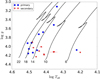 |
Fig. 1. Positions of individual binary components from our sample in Table 1 in the Teff − log g Kiel diagram. Blue squares and red triangles refer to the primary and secondary components, respectively. Evolutionary tracks are computed with solar metallicity Z = 0.014 and for an exponentially decaying CBM profile with fov = 0.02 Hp. Stellar mass is indicated in M⊙ units. |
4. Methodology
In this section, we provide an overview of the adopted methodology, which includes a grid of SSE models. We also discuss the multi-faceted analysis approach in a concise way.
4.1. 1D Stellar evolution models
Even with the computational power currently available, stellar evolution models necessarily remain 1D simplifications of 3D gaseous spheres (e.g. Cristini et al. 2016). The first steps of a solid calibration of stellar interiors from the bridging of 3D simulations and 1D stellar models are being taken from gravity-mode asteroseismology for stars in the mass range of our work (Arnett & Moravveji 2017). The level of sophistication adopted in 1D numerical models of stars with a convective core is diverse, even for the simplest phase of core-hydrogen burning upon which we focus here.
While the simplest of these 1D models rely on mass conservation and on only the pressure force and gravity in the momentum equation, they already suffer from the simplified treatment of convection as a time-independent phenomenon described by at least one free parameter. More complex main-sequence models include any of the Coriolis, Lorentz, and tidal forces, as well as mass loss from a radiation-driven wind (see the monographs by Maeder 2009; Kippenhahn et al. 2012). Moreover, the transport equations to describe the change of the mass fractions of individual chemical elements as a function of time cannot be derived from first principles. These equations include parametrised profiles for the various phenomena of chemical mixing, involving many free parameters, several of which are connected with rotational or magnetic instabilities (e.g. Heger et al. 2000; Palacios 2013). Finally, a variety of choices in numerical implementations to solve the SSE equations and the chosen set of boundary conditions occurs. As a result of these complexities, major differences of orders of magnitude occur in the mixing profiles of stellar models with rotation, as illustrated by comparing Fig. 5 in Chieffi & Limongi (2013) with Fig. 29 in Paxton et al. (2013) and Fig. 3 in Georgy et al. (2013), to list a few.
Consequently, SSE tracks of rotating models in the HR diagram differ a lot. For this reason, we present a complementary approach to the one by Schneider et al. (2014), by investigating the mass-discrepancy problem from non-rotating models guided by recent asteroseismic results. Our sample is ideally suited to perform a calibration of stellar interiors independently from asteroseismology, because it covers well the considered rotation rate of the asteroseismology sample. Just as for asteroseismology of intermediate-mass stars, a good procedure is to assess deviations between the observed diagnostic properties of the binaries in our sample and the theoretical predictions for those diagnostics from 1D models. Given the slow rotation rates of our sample stars and the comparative asteroseismology sample, we consider non-rotating non-magnetic stellar models with extra CBM without pinpointing its physical cause.
4.2. MESA model grid
We rely on a recent grid of MESA models (Paxton et al. 2011, 2013, 2015, 2018, 2019) but extend it towards higher masses compared to the original one presented in Johnston et al. (2019b). The corresponding MESA inlist is optimised for intermediate- and high-mass stars as dictated by the properties of their gravity (g-) mode oscillations. For example, the input physics includes radiative envelope mixing as determined by Rogers & McElwaine (2017) from 2D hydrodynamical simulations of internal gravity waves (IGWs, Rogers et al. 2013) in the form of Denv(r) ∝ ρ−1/2. It has been implemented in MESA in a diffusive approximation by Pedersen et al. (2018) and was shown to have a significant and detectable effect on C, N, and O surface abundances in stars in the mass range under study. Such an envelope mixing profile replaces the default MESA implementation which is assumed to be radially constant and is set by the parameter log Dmix. Though our study does not use any asteroseismic information, it relies on input physics calibrated by most recent asteroseismic findings summarised in Aerts (2019). We use the Ledoux criterion for convection, set the mixing-length parameter αmlt to the solar calibrated value of 1.8, assume a chemical mixture following the cosmic standard for abundances by Przybilla et al. (2008) and Nieva & Przybilla (2012), and set the initial helium and hydrogen fractions to Y = 0.276 and X = 0.71, respectively. The level of envelope mixing near the convective core amounts to log Dmix = 1 cm2 s−1 in our analysis. We refer the reader to Pedersen et al. (2018) and Johnston et al. (2019b) for details on the chosen input physics as well as for the full MESA inlists and RUN_STAR_EXTRAS routines.
Global characteristics of the employed grid of MESA models are summarised in Table 2. We adopt fov = 0.04 and αov = 0.40 as upper limit for the CBM parameter following asteroseismic findings for single stars in the considered mass range (e.g. Aerts 2013, 2019; Pápics et al. 2014; Moravveji et al. 2016; Buysschaert et al. 2018). Even though the grid covers a range in metallicity values, we choose to fix the parameter Z to its solar value (corresponding to 0.014 in mass fraction), consistent with the surface abundances measured from high-resolution spectroscopy for all stars in our sample. By fixing the metallicity and the functional form of the envelope mixing, we restrict ourselves to three free parameters when fitting the position of a star in the Kiel diagram: initial stellar mass M, amount of CBM (fov or αov), and stellar age. Fixing the metallicity of the star also eliminates a number of model degeneracies, in particular the metallicity-initial mass and metallicity-CBM degeneracies. As demonstrated in Fig. 2, lowering the metallicity of the star has a similar effect on the evolutionary track to increasing its initial mass and, to a certain extent, to increasing the CBM level. In all of these cases, evolutionary tracks experience a shift towards higher effective temperatures in the Kiel diagram, while the CBM also leads to an extension of stellar lifetime on the main sequence (left panel in Fig. 2).
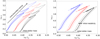 |
Fig. 2. Left: effect of the initial stellar mass M and of an exponentially decaying core-boundary mixing profile with parameter fov on evolutionary tracks. Mass (M = 10 (black), 12 (red), and 15 M⊙ (blue)) and mixing (fov = 0.005 (solid), 0.020 (dashed), and 0.040 Hp (dotted)) sequences are shown with color and line style, respectively. Solar metallicity Z = 0.014 is assumed. Right: effect of the initial stellar mass M and the metallicity Z on evolutionary tracks. The mass sequence is the same as in the left panel; line styles show the metallicity sequence Z = 0.010 (dashed), 0.014 (solid), and 0.018 (dotted) in mass fraction units. A fixed parameter fov = 0.005 Hp is assumed. Note the difference in X, Y-axes in the two panels. |
Summary of the grid of MESA stellar evolution models employed for the analysis of our sample stars.
4.3. Multi-faceted analysis outline
Here, we summarize our multi-faceted analysis approach. The four solutions outlined below are first computed for the single-star scenario assuming no relation between individual binary components, followed by the scenario where both components of a given binary system are forced to have the same age. In either case, we make use of individual stellar masses determined from binary dynamics as a strong observational constraint to report and quantify the mass discrepancy where applicable. Our four solutions are:
Reference model (RM) solution. We fix the initial metallicity Z to the solar value of 0.014 which is consistent with the spectroscopic metallicity measurements for all our targets. At this stage, we ensure the amount of extra near-core mixing is minimal corresponding to fov = 0.005 for the exponentially decaying CBM profile. The effective temperature Teff, surface gravity log g, and (dynamical) stellar mass M are the three parameters that determine the χ2-merit function in this particular case. Given the high precision of the dynamical mass measurements, the solution is largely determined by the mass with less weight given to the Teff and log g parameters. This allows us to form a baseline solution (i.e. reference model) with respect to which the mass discrepancy is quantified in the solution below.
Initial mass (IM) solution. Same as the RM solution except that we exclude the (dynamical) stellar mass from the χ2-merit function, that is, we fitted the position of the star in the Kiel diagram as a constraint. This particular solution allows us to quantify the discrepancy between the measured dynamical mass and the one obtained from fitting the position of the star in the Kiel diagram with stellar evolution models (evolutionary mass, hereafter).
Core boundary mixing (CBM) solution. Same as the RM solution but relaxing the CBM parameter fov, yet including Teff, log g, and the dynamical stellar mass in the χ2-merit function. Similarly to the RM solution case scenario, χ2 is dominated by the dynamical stellar mass due to the high precision of this parameter. However, the fit includes an extra free parameter, which is the amount of near-core mixing.
Initial mass-core boundary mixing (IM-CBM) solution. Same as the IM solution except that the (best fit) CBM parameter fov is adopted (instead of it being fixed it to the minimal value) and the stellar mass is relaxed for those systems where no satisfactory fit could be obtained in the previous solution.
5. Results
In this section, we discuss our results regarding the mass discrepancy across the stellar sample as well as the connection with the near-core mixing. The latter is assumed to have two possible functional forms and associated temperature gradients. The default implementation in MESA is the exponentially decaying efficiency of mixing in the near-core region with radiative temperature gradient, following the prescription of Freytag et al. (1996) and Herwig et al. (1997). An alternative implementation of CBM concerns a step-like functional form with the adiabatic temperature gradient – a prescription that has most often been used in the binary community when addressing the mass discrepancy problem (e.g. Guinan et al. 2000). In this particular case, the near-core region is mixed instantaneously, mimicking the effect of convective penetration and hence implying a global increase in the size and mass of the convective core. The implementation of this penetration formalism in MESA is detailed in Michielsen et al. (2019) to which we refer for details. The extent of the CBM region is parametrised by the fov (αov) parameter in the case of the exponentially decaying and step-like profile, respectively. In the following, the two functional forms of the CBM and their effect on the mass discrepancy are discussed separately.
5.1. Single-star case scenario
As outlined in Sect. 4.3, the mass discrepancy is explored and quantified relative to the reference model, which is detailed in Table 3 (the “RM solution” column). In this model, ages and convective core masses are determined under the assumption of the minimum amount of near-core mixing, using stellar masses measured from binary dynamics. We fail to reproduce the stellar positions in the Kiel diagram for almost the entire sample, with the V578 Mon and U Oph binary systems and the lower mass companion star of V346 Cen being the exceptions. Furthermore, we enforce the dynamical mass values for the primary components of the V380 Cyg and V621 Per systems because of large inconsistencies between their dynamical mass measurements and positions of the stars in the Kiel diagram. Since we fail to reproduce dynamical masses for the majority of the targets with our reference model there is a strong indication of the mass discrepancy and the need for increased core masses in these stars.
The IM solution (cf. Sect. 4.3) quantifies the above discrepancy, with results being detailed in Table 3 and visualised in Fig. 3. We keep the amount of extra near-core mixing at the minimal level and only require the ability to reproduce the position of the star in the Kiel diagram. Satisfactory fits are obtained for all but two stars in our sample, that is, the more massive (primary) components of V380 Cyg and V621 Per. These two stars are by far the most evolved targets in the entire sample with the two lowest surface gravity values (cf. Table 1). The two evident conclusions that can be drawn from Fig. 3 (top row) are: (1) the evolutionary mass of the star is systematically overestimated compared to its dynamical mass and the difference is cumulative with age; and (2) the mass of the convective core of the star follows a similar trend as the stellar mass itself.
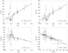 |
Fig. 3. Stellar mass (top left), convective core mass (top right), and stellar age (bottom left) difference between the IM solution (cf. Sect. 4.3 and Table 3, column IM solution) and the RM solution (cf. Sect. 4.3 and Table 3, column RM solution) as a function of stellar surface gravity. The age difference as a function of the stellar mass difference between these two solutions is shown in the bottom right panel. All differences are expressed in percent relative to the RM solution values; the solid line depicts a linear fit in each of the four cases. The Spearman’s rank correlation coefficient (ρ) and the p-value of null hypothesis that there is no correlation between the two sets of variables are listed in each panel. |
The conclusions above are also evidenced by the high absolute values of the Spearman’s rank correlation coefficients ρ and the associated low p-values of the null hypothesis that there is no correlation between the two variables under consideration. Given that the mass of the convective core of non-standard models is regulated by the amount and efficiency of near-core mixing, we investigate this aspect in Sects. 5.1.1 and 5.1.2 in more detail.
It is worth mentioning that the increase of the initial (evolutionary) mass of the star in the IM solution makes the star appear younger (bottom left panel of Fig. 3). We find strong statistical evidence of the effect getting more pronounced the larger the mass discrepancy is (bottom right panel of Fig. 3). Finally, we also note that the above mentioned (more massive) primary components of the V380 Cyg and V621 Per systems are not shown in Fig. 3 as their positions in the Kiel diagram could not be reproduced in the IM solution. These findings are in line with the conclusions by Tkachenko et al. (2014) who find that increasing the initial stellar mass in evolutionary models alone is not sufficient to remedy the mass discrepancy for the more evolved primary component of V380 Cyg. Here, we find the same result for the primary component of V621 Per as well.
5.1.1. CBM in the diffusive exponentially decaying approximation
Given the strong link between the mass discrepancy and the mass of the convective core of the star, we explore further a probable connection of the effect with the amount and efficiency of the near-core mixing. The CBM solution (cf. Sect. 4.3) aims to reproduce stellar positions in the Kiel diagram under the assumption of their dynamical masses while allowing for a variable parameter fov in an exponentially decaying CBM profile. The CBM solution is different from the RM solution in that we relax this parameter, letting the mass of the convective core increase due to the enhanced mixing in the near-core regions, while keeping a tight constraint on the total mass.
The CBM solution is detailed in Table 3 (the “CBM solution” column) where the convergence towards the upper grid limit of the fov parameter is immediately evident for almost the entire stellar sample. This is not an unexpected outcome given the extra supply of fresh hydrogen to the convective core and the associated increase in core mass. In that sense, the CBM (to a certain extent) mimics the effect of varying initial stellar mass, which is central to the stellar mass-CBM degeneracy discussed in Sect. 4.2 (cf. Fig. 2). Indeed, comparison with the RM solution (reference model) values in the left column of Fig. 4 demonstrates that: (1) the mass of the convective core of the star increases with the inclusion of extra CBM in stellar evolution models, and the increase is a clear function of the surface gravity of the star (top left panel with p below 0.001); and (2) all stars get systematically older with the inclusion of CBM (bottom left panel), which is again expected given that more near-core mixing implies an increase of the stellar lifetime on the main sequence. This was already represented in the isochrone clouds in Johnston et al. (2019b).
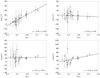 |
Fig. 4. Convective core mass (top row) and age (bottom row) changes due to the inclusion of extra near-core mixing in the models (cf. Table 3, column CBM solution). Left and right columns: comparisons against the RM solution (cf. Sect. 4.3 and Table 3, column RM solution) and the IM solution (cf. Sect. 4.3 and Table 3, column IM solution), respectively. |
The right column of Fig. 4 compares the best CBM solution with the one that assumes a minimum amount of the near-core mixing but allows for a variable initial stellar mass (the IM solution; cf. Sect. 4.3 and the “IM solution” column in Table 3). One can clearly see from the top right panel in Fig. 4 that there is no significant difference between the obtained convective core masses (p exceeding 0.99), strengthening our claim that allowing the CBM parameter to vary is equivalent to allowing the initial mass to vary. The fov parameter has a non-negligible effect on stellar age as we find our sample to be systematically older. There is also a weak indication of the age difference increasing with the surface gravity of the star (bottom right panel with p < 0.25).
An important observation from Table 3 (the “CBM solution” column) is that the positions of stars in the Kiel diagram of only about half of our sample stars are well reproduced with a variable CBM parameter. The remaining half of the sample either requires more mass in the convective core at a given age of the star or a younger age. In other words, the mass discrepancy problem appears to be a combined effect of the age and the mass of the convective core of the star in stellar evolution models. The above is demonstrated in our IM-CBM solution (cf. Sect. 4.3) where we adopt the best fit value of the fov parameter from the previous solution and relax stellar mass for systems that could not be fitted with variable CBM alone. Increasing the initial mass of the star makes its core slightly more massive and it makes the star younger at its (fixed) position in the Kiel diagram. This particular combination allows us to reproduce the atmospheric parameters for the remainder of the sample, including the primary components of V621 Per and V380 Cyg – the two most evolved stars in our sample.
Our solution is detailed in Table 3 (the “IM-CBM solution” column) and is compared with the IM and CBM solutions in the left and right columns of Fig. 5, respectively. The primary components of V621 Per and V380 Cyg are not included in the comparison because the IM solution did not reveal satisfactory fits for both stars and the mass discrepancy could not be quantified for them. One can see that the convective core mass has generally increased by ∼5−10% (top left panel) while the stars have generally become older (bottom left panel) compared to the IM solution. One also notices a strong negative correlation between the increase of the convective core mass and surface gravity of the star (p < 0.001), while the relationship for the age difference is not statistically significant (p > 0.99). At the same time, the sample is generally younger than the CBM solution (bottom right panel), yet the increase in the convective core mass is evident (top right panel). A noteworthy feature in the right panels of Fig. 5 is the two populations of stars – those clustering at zero value on the ordinate axis and rest of the sample. This bimodality is simply the result of adopting the exact parameters from the CBM solution for stars whose atmospheric properties and dynamical masses are reproduced with extra amount of the near-core mixing and did not require any further change of the initial mass in stellar evolution models. In other words, these are the systems that no longer show the mass discrepancy after introducing the exponentially decaying CBM in a diffusive approximation with the free parameter fov.
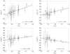 |
Fig. 5. Same as Fig. 4 but for the IM-CBM solution (cf. Sect. 4.3 and Table 3, column IM-CBM solution). Left and right columns: comparison against the IM (cf. Table 3, column IM solution) and CBM (cf. Table 3, column CBM solution) solutions, respectively. |
Finally, Fig. 6 (left panel) shows the mass discrepancy as a function of the surface gravity of the star, where the discrepancy is determined with respect to the dynamical mass of the star. Similar to the previous case, two stellar populations are evident: (1) stars clustering at the zero mass discrepancy have positions in the Kiel diagram that are well reproduced by adopting their dynamical masses in combination with extra near-core mixing (cf. CBM solution); and (2) the rest of the sample requires higher evolutionary masses in addition to the CBM to reproduce the atmospheric properties of the respective stars. For this latter sub-sample, the mass discrepancy amounts to some 10% on average with no statistically significant dependence on the surface gravity of the star. The two most evolved stars in the sample are the primary components of V621 Per and V380 Cyg, which are also included in Fig. 6 and show a mass discrepancy ΔM ∼ 25% and ∼30%, respectively. The mass discrepancy for the other 19 stars is reduced compared to the case of minimum amount of the near-core mixing (cf. the IM solution), which is evidenced by the right panel of Fig. 6. Just as the mass discrepancy itself, the reduction is the largest for more evolved stars, that is, those with the lowest measured surface gravities.
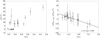 |
Fig. 6. Left: remaining mass discrepancy after introducing an exponentially decaying CBM profile with radiative temperature gradient (the IM-CBM solution, cf. Sect. 4.3 and respective column in Table 3), defined as percentage of the dynamical mass of the star. Right: percentage difference between the mass discrepancy after (the IM-CBM solution) and before (the IM solution) the inclusion of CBM in the models. |
5.1.2. Step-like CBM with instantaneous mixing
Subsequently, we test a different functional form of the CBM, having a different temperature gradient in that zone. More precisely, the exponentially decaying formalism is replaced with a step function with the temperature gradient in the near-core region also changed from radiative to fully adiabatic (i.e. convective penetration; Zahn 1991). The results corresponding to this form of CBM are summarised in Table 4, while Fig. 7 shows a comparison between the two functional forms of the CBM. Left and right panels show the change of the convective core mass and age, respectively, where the parameter in question corresponding to the exponential functional form is subtracted from the one based on the step formalism. One can see that there is no statistically significant change in the age of the stellar sample while the mass of the convective core is consistently lower by about 5−10%. As evidenced by p > 0.99, neither the mass of the convective core nor the age of the star show any significant correlation with stellar surface gravity.
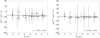 |
Fig. 7. Relative change in the convective core mass (left) and age (right) of the star between solutions assuming a step-like and an exponentially decaying functional form of the CBM. The Y-axes are in percent relative to the value dictated by the solution with the exponentially decaying CBM. |
Similarly to the case of the exponentially decaying CBM, we reach the upper grid limit for the αov parameter in the majority of cases, as evidenced from Table 4. The two parameters, fov and αov, differ by a factor of ten for almost all stars in the sample (the IM solution column in Tables 3 and 4). The fact that we do not reach the same mass of the convective core in the case of the αov parameter suggests a somewhat larger conversion factor between the parametrisations, when interpreted in terms of efficiency of the mixing as to increasing the mass of the convective core. This is fully consistent with Claret & Torres (2017), who found the scaling αov/fov = 11.36 ± 0.22 based on their study of 56 individual stellar components of binary systems, while earlier studies by Moravveji et al. (2016) and Valle et al. (2017) suggested αov/fov ≈ 13 and 12, respectively.
5.2. Binary equal age-case scenario
So far, our results have been obtained under the assumption that the individual stellar components are single stars with their masses and surface gravities being obtained in a model-independent way. In reality, they are members of binary star systems which puts further strong constraints on stellar evolution models, namely that both components of a binary system should have the same age.
In this section, we repeat the sequence of analyses outlined in Sect. 4.3 for the single-star case scenario in Sect. 5.1, but also forcing an equal age condition for both stellar components of each binary system in the sample. The obtained results are summarised in Table A.1 in columns designated RM, IM, CBM, and IM-CBM solutions and in Figs. A.1–A.4. The distributions look somewhat different from those for the single star-case scenario due to some systems showing considerably different ages for their individual stellar components (e.g. AH Cep in Table 3, the RM solution column). Enforcing the equal-age condition for these systems propagates into the other free parameters in the fitting, like initial mass and amount of near-core mixing. This results in unsatisfactory fits for a total of four stellar components (primary/secondary component of the V380 Cyg/V346 Cen system and both components of V573 Car) in our ultimate IM-CBM solution (cf. Table A.1) compared to none in the single star-case scenario. Figures A.1–A.4 confirm our main conclusions from Sect. 5.1 that: (1) the (convective core) mass discrepancy tends to increase as the surface gravity of the star decreases; (2) the mass discrepancy can be partially accounted for by increasing the amount of the near-core mixing and the mass of the convective core; and (3) because of the link between the mass discrepancy and stellar age, the near-core mixing should not be increased infinitely as it makes the star older with increasing convective core mass. For this reason, we have limited the fov and αov values to those covered from asteroseismic inference of single pulsators in the mass regime under study (for both convective penetration and diffusive exponential CBM; Aerts 2019).
6. Revisiting the case of V380 Cyg
As discussed in the previous sections, the primary components of V380 Cyg and V621 Per are by far the most evolved stars in our sample. We consider the evolved primary component of the V380 Cyg system as representative of the class in this section and provide a possible scenario of why the mass discrepancy shows a strong negative correlation with the surface gravity of the star. A notable characteristic of the primary component of V380 Cyg is its high value of the required microturbulent velocity ξ = 15 ± 1 km s−1 as measured by Tkachenko et al. (2014) from high-resolution optical spectra. Having high values of the microturbulent velocity is a common phenomenon in massive evolved stars as demonstrated by Cantiello et al. (2009) from samples of high-mass stars in the Galaxy and in the LMC. The authors also report a strong anti-correlation between the observed microturbulent velocities and stellar surface gravities, namely ξ tends to increase as log g decreases. This is related to the formation of a sub-surface convection zone in high-mass stars that gives rise to the microturbulent velocity field. Microturbulence results predominantly in radial velocities and accompanying spectral line variations and should not be confused with macroturbulent broadening, which requires horizontal velocities to be dominant over radial ones in the line-forming region. A connection between macroturbulent line broadening and the horizontal velocities due to internal gravity waves has been suggested (Aerts & Rogers 2015).
In this section, we take a closer look at the problem of high microturbulence in the primary component of V380 Cyg and discuss it in the context of the mass discrepancy problem. Standard spectrum analysis procedures are based on grids of pre-computed atmosphere models that are fed into spectrum synthesis algorithms to allow comparison between observed and theoretical spectra in arbitrary wavelength intervals. Though spectral synthesis algorithms often allow for optimisation of all fundamental atmospheric parameters of stars, including the microturbulent velocity parameter ξ, atmosphere model grids are typically available for only a few values of microturbulent velocity, with ξ = 2 km s−1 being the most commonly adopted value. A similar approach was also used by Tkachenko et al. (2014), where the authors adopted the grid of ξ = 2 km s−1 ATLAS9 models (Kurucz 1993) and determined the optimal microturbulent velocity along with other atmospheric parameters, by varying it in the spectrum synthesis code. Despite the large inconsistency between the derived microturbulent velocity of ξ = 15 ± 1 km s−1 from the observed spectrum and ξ = 2 ± 1 km s−1 adopted in the ATLAS9 atmosphere models, no further iterations have been done to maintain self-consistency in the spectrum analysis procedure.
Including microturbulence in stellar atmosphere models leads to an increase of the turbulent pressure, which in turn impacts the gas pressure to meet the condition of total pressure conservation. This alters the temperature at a given optical depth, hence influencing the entire structure of the stellar atmosphere model. We demonstrate this effect in Fig. 8 (left panel) where the temperature difference between atmosphere models with ξ = 15 km s−1 and ξ = 2 km s−1 is plotted as a function of the logarithm of the Rosseland optical depth. For these calculations (performed with the LLMODELS stellar atmosphere model code; Shulyak et al. 2004), we assume an atmosphere model corresponding to the primary component of V380 Cyg, that is Teff = 21 500 K, log g = 3.1 dex, and [M/H] = 0.0 dex. One can see that the temperature difference associated with an increase of microturbulence and inclusion of turbulent pressure is significant in the line forming regions, and unavoidably affects both shapes and strengths of individual lines in the stellar spectrum. The latter effect is illustrated in the right panel of Fig. 8, where we plot stellar spectra synthesised with the GSSP code from atmosphere models with ξ = 15 km s−1 (dashed red line) and with ξ = 2 km s−1 (solid black line), along with their difference (dotted blue line), where the latter is subtracted from the former. We also added a Gaussian noise to both spectra to simulate S/N ∼ 100 for a realistic illustration.
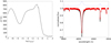 |
Fig. 8. Left: temperature difference between a model atmosphere computed with a microturbulent velocity of ξ = 15 and 2 km s−1, as a function of the logarithm of the Rosseland optical depth. Right: differences in spectral line profiles associated with the change of microturbulent velocity in the model atmosphere from ξ = 2 km s−1 (solid black line) to ξ = 15 km s−1 (dashed red line). The difference spectrum (dotted blue line) was vertically shifted for clarity. Gaussian noise was added to both spectra to simulate a signal-to-noise ratio S/N ∼ 100. |
Analyzing the spectrum of a hot star where spectral lines are altered by a significant contribution from turbulent pressure with a grid of ξ = 2 km s−1 atmosphere models leads to large systematic uncertainties in parameters such as Teff and log g. Given that the latter parameter is computed from the dynamical mass and radius in the case of binary stars, Teff is the parameter that suffers the most. In order to illustrate this quantitatively, we employ a grid of ξ = 2 km s−1 atmosphere models to analyze the spectrum shown with the solid black line in Fig. 8 and having the following parameters: Teff = 21 500 K, log g = 3.1 dex, ξmodel = 15 km s−1, ξspectrum = 15 km s−1, [M/H] = 0.0 dex, and v sin i = 100 km s−1. In this process, we keep log g fixed to 3.1 dex assuming it is known from the dynamical mass and radius of the star. The obtained best fit parameters are: Teff = 23 190 ± 210 K, ξspectrum = 14.1 ± 1.0 km s−1, [M/H] = −0.01 ± 0.05 dex, and v sin i = 98.5 ± 3.4 km s−1. One can see that, though the other parameters agree with their input values within 1σ uncertainties, Teff is overestimated by ∼1700 K, that is, some 8%.
The left panel of Fig. 9 shows MESA evolutionary tracks corresponding to four single-star-case scenario solutions detailed in Table 3. One can see that the tracks corresponding to the dynamical masses of the stars (11.43 ± 0.19 M⊙ and 7.00 ± 0.14 M⊙ for the primary and secondary, respectively) are significantly off from their spectroscopic positions and that increasing near-core mixing does not solve the problem. It is essential to introduce a mass discrepancy of ∼30% (∼20%) for the primary (secondary) component to maintain consistency between evolutionary tracks and spectroscopically measured parameters, where a high value of the parameter fov ≈ 0.04 Hp is also essential to use for the more evolved primary. The mass discrepancy gets substantially reduced when Teff of the primary is corrected by 8% of the measured value in order to account for the effect of the microturbulent velocity in the stellar atmosphere model (Fig. 9, right panel). In practice, the mass discrepancy nearly vanishes for the primary of V380 Cyg when its dynamical mass and high fov are assumed. The argument of microturbulence in atmosphere models does not apply to the secondary component of V380 Cyg as it is an unevolved star. However, using a wrong value for Teff for the primary has a significant effect on determining Teff of the low flux contributing secondary, both in the spectrum analysis of the disentangled spectra and in the photometric analysis of the light curve. Indeed, Tkachenko et al. (2014) report a significant difference of ∼2000 K between spectroscopic and photometric values of Teff for the secondary and adopt the mean value as a compromise. It is essential to perform a full re-analysis of the system in a self-consistent way in order to answer the question whether accounting for the effect of microturbulence in atmosphere models and of missing convective core mass in SSE models resolves the mass discrepancy for V380 Cyg.
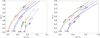 |
Fig. 9. Left: four solutions obtained for the V380 Cyg system and detailed in Table 3. The corresponding MESA evolutionary tracks are shown with solid (dashed) lines for the primary (secondary) component. The RM, IM, CBM, and IM-CBM solutions are shown in black, red, blue, and green, respectively. The more (less) evolved primary (secondary) is shown with filled square (triangle) symbols. Right: changing position of the primary component (open square) associated with a reduced Teff by 8%. The color coding is the same as in the left panel. |
Stellar evolution dictates the formation of a sub-surface convection zone in high-mass stars as they approach the Terminal Age Main-Sequence (TAMS), giving rise to a higher microturbulent velocity field (e.g., Cantiello et al. 2009). Ignoring the effect of microturbulence by fixing it to 2 km s−1 in stellar atmosphere models implies overestimation of the effective temperature of the star by means of a spectroscopic analysis. As demonstrated in Figs. 2 and 9, increasing the initial mass of the star in stellar evolution models shifts the corresponding track to higher temperatures (Fig. 2, left panel). Hence, one introduces the mass discrepancy by overestimating the effective temperature of the star and the effect is expected to be more pronounced for evolved main-sequence stars. The latter correlation in terms of the dependence of the mass discrepancy on the surface gravity of the star is exactly what we find in our stellar sample (see, e.g. top left panels in Figs. 3 and A.1).
7. Discussion and conclusions
In this paper, we presented the mass discrepancy problem as observed in intermediate- and high-mass eclipsing SB2 binary stars. Discovered in a large sample of single stars (Herrero et al. 1992), the problem obtained further acknowledgement in the stellar astrophysics community when it was observed in binary stars, largely because of the model-independent way of measuring accurate stellar masses and radii in such systems. A common proposed solution to the mass discrepancy problem until now was a significant increase of near-core mixing in the form of convective core overshooting, either adopting a step formalism with an adiabatic temperature gradient (e.g. Guinan et al. 2000) or an exponentially decaying diffusive mixing with a radiative temperature gradient in the overshoot zone (e.g. Tkachenko et al. 2014).
In order for the mass discrepancy problem to be properly addressed, a homogeneously analysed sample of binary stars whose components cover a large range in stellar mass and evolutionary stage is needed. This avoids systematic uncertainties propagating into the analysis of the problem, hence influencing conclusions in a largely unpredictable way. Our stellar sample is the first that meets the homogeneity requirement and comprises eleven eclipsing SB2 binary systems, whose individual stellar components are slow to moderate rotators covering the mass range from M ≈ 4.5 M⊙ to M ≈ 17 M⊙ and evolutionary stage from the ZAMS to the TAMS. The analysis is performed both in the single-star scenario where the binary components are treated independent of each other, and in the binary-star scenario where we enforce the equal-age condition for the two stellar components of the same binary system. The results of these two analyses are qualitatively alike and can be summarised as follows:
-
the mass discrepancy is clearly present in our stellar sample and there is strong statistical evidence (p < 0.01) of it being anti-correlated with surface gravity;
-
a strong relationship exists between the convective core mass and the mass discrepancy. More precisely, there is strong evidence that SSE models without extra near-core mixing underestimate the convective core mass. Statistical evidence is found that the problem becomes more pronounced as the star evolves during the main-sequence;
-
because of its ability to supply the convective core with fresh hydrogen and to increase its mass, enhanced near-core boundary mixing can partially account for the observed mass discrepancy. The mass discrepancy turns out to be a convective core mass–stellar age correlation/problem in stellar evolution models;
-
the mass discrepancy does not correlate with any other fundamental or atmospheric parameters of stars than their surface gravity (proxy for age/low density atmosphere);
-
neglecting high microturbulent velocity values and turbulent pressure in stellar atmosphere models of hot stars results in an overestimation of the effective temperature of a star up to some 8%, when its dynamical log g value is assumed. This effect is larger for more evolved stars, that is, those that show lower surface gravities and are located closer to the TAMS. In practice, stars appear hotter than they are, which partially contributes to the mass discrepancy problem.
We conclude that the mass discrepancy problem in binary stars is the combined effect of a convective core mass-stellar age correlation in stellar evolution models and the neglect of high microturbulent velocities and turbulent pressure in stellar atmosphere models in spectroscopic analysis.
Claret & Torres (2016, 2017, 2018, 2019) report an almost linear increase of the overshooting parameter αov(fov) from 0.0 Hp to ∼0.2 (0.02) Hp for masses between M ≈ 1.2 M⊙ and M ≈ 2.0 M⊙ and report systematically lower metallicities from stellar evolution models compared to values inferred from high-resolution spectroscopy. In their work, the authors suggest that the initially adopted lower helium abundance Y = 0.24 is most likely the cause of the observed effect (Claret & Torres 2017). In Sect. 4.2 (cf. Fig. 2, right panel), we demonstrated that lowering the initial metallicity parameter Z in stellar evolution models has a similar effect to increasing the initial mass of a star. We estimate that for a M = 2.5 M⊙ star (approximately at the center of the stellar mass range studied by Claret & Torres 2016), the effect of decreasing the metallicity parameter from Z = 0.014 to Z = 0.010 (0.006) is similar to the effect of increasing the initial stellar mass by 0.25 (0.35) M⊙, that is, 10 (15)% of the assumed value of M = 2.5 M⊙. Hence, the low metallicity values dictated by stellar evolution models for about half of the sample studied in Claret & Torres (2016, 2017, 2019) can also be the manifestation of the mass discrepancy problem in binary stars born with a convective core. This moderate mass discrepancy gets compensated by a moderate increase of the mass of the convective core of the star that is provided by enhanced near-core boundary mixing. We find low parameter values fov = 0.013 ± 0.013 and fov = 0.017 ± 0.012 for the primary and secondary component of the U Oph system, the two lowest-mass stars in our sample with M = 5.10 ± 0.05 M⊙ and M = 4.60 ± 0.05 M⊙, respectively.
There is a substantial overlap between targets in our sample and stars investigated by Schneider et al. (2014), yet a quantitative comparison between the two studies proves difficult. While Schneider et al. (2014) adopted parameters from the catalogue by Torres et al. (2010), we reanalysed all the targets in a homogeneous way to avoid systematic uncertainties, so that the parameters can in some cases differ substantially between the two studies. As a particular example, we find the primary component of AH Cep to be about 6% more massive, while both components of the V478 Cyg system are ∼1300 K hotter compared to the values adopted by Schneider et al. (2014). Additionally, these authors adopted a grid of stellar evolution models computed for a lower metallicity Z = 0.0088 (though with an increased iron abundance so that it closely resembles the solar value of log(Fe/H) + 12 ≈ 7.50), while we adopt a metallicity of Z = 0.014, which is in agreement with the spectroscopic analyses of the stars in our sample.
Finally, we point out that the two single B-type stars with asteroseismic estimations of their Mcc/M have values of 21% (Moravveji et al. 2015) and 19% (Moravveji et al. 2016), both having a mass of M ≃ 3.2 M⊙. This is very much in line with our results for the binaries. To illustrate the importance of extra CBM, we plot Mcc/M versus M for our sample stars in Fig. 10, color coded according to veq/vcrit (left panel) and main-sequence phase according to Xc (right panel). It can be seen that Mcc/M steadily increases as M increases, as expected from SSE theory. We also find that there is no correlation between the rotation rate and Mcc/M. Further, it can be seen that all the stars in our sample, including the most evolved ones, have Mcc/M far above the value predicted by SSE models with minimal CBM (dashed line). The results of our work on Mcc/M, graphically represented in Fig. 10, imply that stars have much larger helium cores near the TAMS compared to SSE models with no extra near-core mixing.
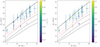 |
Fig. 10. Convective core mass as a function of total mass for ZAMS models (full line) and models for the central hydrogen mass fractions of Xc = 0.35 (red) and Xc = 0.1 (black) when considering low (dashed), moderate (dashed-dot), and high (dotted) levels of CBM according to the ranges in Table 2. The sample stars are added with color coding according to their veq/vcirt (left) and their Xc (right). |
In the future, we plan to increase the size of our stellar sample drastically by extending it towards both lower and higher masses. It is important to keep the sample homogeneous in terms of data analysis to make sure systematic uncertainties associated with the use of different algorithms do not propagate to final conclusions. Higher-mass stars than those in our current sample tend to have strong winds driving significant mass loss from the star. In this case, using our suite of analysis techniques is not justified anymore. Furthermore, it would be important to revisit some of the systems like V380 Cyg. As we have shown in this study, it is essential to take into account the high microturbulent velocity and turbulent pressure in atmosphere model calculations of such stars. In this context, it is also important to balance our sample by including more stars at advanced stages of (main-sequence) evolution, from mid main-sequence onwards. Last but not least, searching for eclipsing, spectroscopic double-lined binary systems with stellar components pulsating in gravity-mode oscillations is another promising step forward in calibrating stellar evolution models with binary stars (Aerts 2019). Space-missions such as TESS (Ricker et al. 2015) and PLATO (Rauer et al. 2014) are excellent observational facilities to search for the best candidate asteroseismic binary systems.
Acknowledgments
The research leading to these results has received funding from the European Research Council (ERC) under the European Union’s Horizon 2020 research and innovation programme (grant agreement N°670519: MAMSIE), from the KU Leuven Research Council (grant C16/18/005: PARADISE), from the Research Foundation Flanders (FWO) under grant agreements G0H5416N (ERC Runner Up Project) and G0A2917N (BlackGEM), as well as from the BELgian federal Science Policy Office (BELSPO) through PRODEX grant PLATO. KP acknowledges financial support from the Croatian Science Foundation under grant IP-2014-09-8656 (STARDUST). VT acknowledges support by the RF Ministry of Science and Higher Education in the framework of the state task (project no. 3.7126.2017/8.9).
References
- Aerts, C. 2013, EAS Pub. Ser., 64, 323 [CrossRef] [Google Scholar]
- Aerts, C. 2019, Rev. Mod. Phys., submitted [arXiv:1912.12300] [Google Scholar]
- Aerts, C., & Rogers, T. M. 2015, ApJ, 806, L33 [NASA ADS] [CrossRef] [Google Scholar]
- Aerts, C., Molenberghs, G., Michielsen, M., et al. 2018, ApJS, 237, 15 [NASA ADS] [CrossRef] [Google Scholar]
- Aerts, C., Mathis, S., & Rogers, T. M. 2019, ARA&A, 57, 35 [NASA ADS] [CrossRef] [MathSciNet] [Google Scholar]
- Arnett, W. D., & Moravveji, E. 2017, ApJ, 836, L19 [NASA ADS] [CrossRef] [Google Scholar]
- Borucki, W. J., Koch, D., Basri, G., et al. 2010, Science, 327, 977 [NASA ADS] [CrossRef] [PubMed] [Google Scholar]
- Bowman, D. M., Johnston, C., Tkachenko, A., et al. 2019, ApJ, 883, L26 [NASA ADS] [CrossRef] [Google Scholar]
- Butler, K. 1984, PhD Thesis, University College London [Google Scholar]
- Buysschaert, B., Aerts, C., Bowman, D. M., et al. 2018, A&A, 616, A148 [NASA ADS] [CrossRef] [EDP Sciences] [Google Scholar]
- Cantiello, M., Langer, N., Brott, I., et al. 2009, A&A, 499, 279 [NASA ADS] [CrossRef] [EDP Sciences] [Google Scholar]
- Chaplin, W. J., Basu, S., Huber, D., et al. 2014, ApJS, 210, 1 [NASA ADS] [CrossRef] [Google Scholar]
- Chieffi, A., & Limongi, M. 2013, ApJ, 764, 21 [NASA ADS] [CrossRef] [Google Scholar]
- Christensen-Dalsgaard, J. 2002, Rev. Mod. Phys., 74, 1073 [NASA ADS] [CrossRef] [Google Scholar]
- Christensen-Dalsgaard, J., & Gough, D. O. 1976, Nature, 259, 89 [NASA ADS] [CrossRef] [Google Scholar]
- Claret, A. 1995, A&AS, 109, 441 [NASA ADS] [Google Scholar]
- Claret, A. 2004, A&A, 424, 919 [NASA ADS] [CrossRef] [EDP Sciences] [Google Scholar]
- Claret, A. 2012, A&A, 541, A113 [NASA ADS] [CrossRef] [EDP Sciences] [Google Scholar]
- Claret, A., & Torres, G. 2016, A&A, 592, A15 [NASA ADS] [CrossRef] [EDP Sciences] [Google Scholar]
- Claret, A., & Torres, G. 2017, ApJ, 849, 18 [NASA ADS] [CrossRef] [Google Scholar]
- Claret, A., & Torres, G. 2018, ApJ, 859, 100 [NASA ADS] [CrossRef] [Google Scholar]
- Claret, A., & Torres, G. 2019, ApJ, 876, 134 [Google Scholar]
- Claverie, A., Isaak, G. R., McLeod, C. P., van der Raay, H. B., & Cortes, T. R. 1979, Nature, 282, 591 [NASA ADS] [CrossRef] [Google Scholar]
- Costa, G., Girardi, L., Bressan, A., et al. 2019, MNRAS, 485, 4641 [NASA ADS] [CrossRef] [Google Scholar]
- Cristini, A., Meakin, C., Hirschi, R., et al. 2016, Phys. Scr., 91, 034006 [NASA ADS] [CrossRef] [Google Scholar]
- Daszyńska-Daszkiewicz, J., & Miszuda, A. 2019, ApJ, 886, 35 [NASA ADS] [CrossRef] [Google Scholar]
- Duvall, T. L., Jr., & Harvey, J. W. 1983, Nature, 302, 24 [NASA ADS] [CrossRef] [Google Scholar]
- Eggenberger, P., Deheuvels, S., Miglio, A., et al. 2019a, A&A, 621, A66 [NASA ADS] [CrossRef] [EDP Sciences] [Google Scholar]
- Eggenberger, P., den Hartogh, J. W., Buldgen, G., et al. 2019b, A&A, 631, L6 [NASA ADS] [CrossRef] [EDP Sciences] [Google Scholar]
- Ekström, S., Meynet, G., Maeder, A., & Barblan, F. 2008, A&A, 478, 467 [NASA ADS] [CrossRef] [EDP Sciences] [Google Scholar]
- Evans, J. W., & Michard, R. 1962a, ApJ, 135, 812 [NASA ADS] [CrossRef] [Google Scholar]
- Evans, J. W., & Michard, R. 1962b, ApJ, 136, 487 [NASA ADS] [CrossRef] [Google Scholar]
- Evans, J. W., & Michard, R. 1962c, ApJ, 136, 493 [NASA ADS] [CrossRef] [Google Scholar]
- Freytag, B., Ludwig, H. G., & Steffen, M. 1996, A&A, 313, 497 [NASA ADS] [Google Scholar]
- Fuller, J. 2017, MNRAS, 472, 1538 [NASA ADS] [CrossRef] [Google Scholar]
- Fuller, J., Piro, A. L., & Jermyn, A. S. 2019, MNRAS, 485, 3661 [NASA ADS] [Google Scholar]
- Garcia, E. V., Stassun, K. G., Pavlovski, K., et al. 2014, AJ, 148, 39 [NASA ADS] [CrossRef] [Google Scholar]
- Georgy, C., Ekström, S., Granada, A., et al. 2013, A&A, 553, A24 [NASA ADS] [CrossRef] [EDP Sciences] [Google Scholar]
- Giddings, J. R. 1981, PhD Thesis, University College London [Google Scholar]
- Gough, D. O., Leibacher, J. W., Scherrer, P. H., & Toomre, J. 1996, Science, 272, 1281 [NASA ADS] [CrossRef] [Google Scholar]
- Guinan, E. F., Ribas, I., Fitzpatrick, E. L., et al. 2000, ApJ, 544, 409 [NASA ADS] [CrossRef] [Google Scholar]
- Guo, Z., Gies, D. R., & Fuller, J. 2017, ApJ, 834, 59 [NASA ADS] [CrossRef] [Google Scholar]
- Guo, Z., Fuller, J., Shporer, A., et al. 2019, ApJ, 885, 46 [NASA ADS] [CrossRef] [Google Scholar]
- Hambleton, K., Degroote, P., Conroy, K., et al. 2013a, EAS Pub. Ser., 64, 285 [CrossRef] [Google Scholar]
- Hambleton, K. M., Kurtz, D. W., Prša, A., et al. 2013b, MNRAS, 434, 925 [NASA ADS] [CrossRef] [MathSciNet] [Google Scholar]
- Harvey, J. W., Hill, F., Hubbard, R. P., et al. 1996, Science, 272, 1284 [NASA ADS] [CrossRef] [PubMed] [Google Scholar]
- Heger, A., Langer, N., & Woosley, S. E. 2000, ApJ, 528, 368 [NASA ADS] [CrossRef] [Google Scholar]
- Hekker, S., & Christensen-Dalsgaard, J. 2017, A&ARv, 25, 1 [NASA ADS] [CrossRef] [EDP Sciences] [Google Scholar]
- Herrero, A., Kudritzki, R. P., Vilchez, J. M., et al. 1992, A&A, 261, 209 [NASA ADS] [Google Scholar]
- Herwig, F., Bloecker, T., Schoenberner, D., & El Eid, M. 1997, A&A, 324, L81 [NASA ADS] [Google Scholar]
- Higl, J., & Weiss, A. 2017, A&A, 608, A62 [NASA ADS] [CrossRef] [EDP Sciences] [Google Scholar]
- Ilijic, S., Hensberge, H., Pavlovski, K., & Freyhammer, L. M. 2004, ASP Conf. Ser., 318, 111 [NASA ADS] [Google Scholar]
- Johnston, C., Pavlovski, K., & Tkachenko, A. 2019a, A&A, 628, A25 [NASA ADS] [CrossRef] [EDP Sciences] [Google Scholar]
- Johnston, C., Tkachenko, A., Aerts, C., et al. 2019b, MNRAS, 482, 1231 [NASA ADS] [CrossRef] [Google Scholar]
- Kippenhahn, R., Weigert, A., & Weiss, A. 2012, Stellar Structure and Evolution (Berlin, Heidelberg: Springer-Verlag) [Google Scholar]
- Kurucz, R. 1993, ATLAS9 Stellar Atmosphere Programs and 2 km/s grid. Kurucz CD-ROM No. 13 (Cambridge, Mass.: Smithsonian Astrophysical Observatory), 13 [Google Scholar]
- Lastennet, E., & Valls-Gabaud, D. 2002, A&A, 396, 551 [NASA ADS] [CrossRef] [EDP Sciences] [Google Scholar]
- Leighton, R. B., Noyes, R. W., & Simon, G. W. 1962, ApJ, 135, 474 [NASA ADS] [CrossRef] [Google Scholar]
- Maeder, A. 2009, Physics, Formation and Evolution of Rotating Stars (Berlin, Heidelberg: Springer) [Google Scholar]
- Michielsen, M., Pedersen, M. G., Augustson, K. C., Mathis, S., & Aerts, C. 2019, A&A, 628, A76 [NASA ADS] [CrossRef] [EDP Sciences] [Google Scholar]
- Moravveji, E., Aerts, C., Pápics, P. I., Triana, S. A., & Vandoren, B. 2015, A&A, 580, A27 [NASA ADS] [CrossRef] [EDP Sciences] [Google Scholar]
- Moravveji, E., Townsend, R. H. D., Aerts, C., & Mathis, S. 2016, ApJ, 823, 130 [NASA ADS] [CrossRef] [MathSciNet] [Google Scholar]
- Nieva, M.-F., & Przybilla, N. 2012, A&A, 539, A143 [NASA ADS] [CrossRef] [EDP Sciences] [Google Scholar]
- Palacios, A. 2013, EAS Pub. Ser., 62, 227 [CrossRef] [Google Scholar]
- Pápics, P. I., Moravveji, E., Aerts, C., et al. 2014, A&A, 570, A8 [NASA ADS] [CrossRef] [EDP Sciences] [Google Scholar]
- Pavlovski, K., & Southworth, J. 2009, MNRAS, 394, 1519 [NASA ADS] [CrossRef] [Google Scholar]
- Pavlovski, K., Tamajo, E., Koubský, P., et al. 2009, MNRAS, 400, 791 [NASA ADS] [CrossRef] [Google Scholar]
- Pavlovski, K., Southworth, J., & Tamajo, E. 2018, MNRAS, 481, 3129 [NASA ADS] [Google Scholar]
- Paxton, B., Bildsten, L., Dotter, A., et al. 2011, ApJS, 192, 3 [Google Scholar]
- Paxton, B., Cantiello, M., Arras, P., et al. 2013, ApJS, 208, 4 [NASA ADS] [CrossRef] [Google Scholar]
- Paxton, B., Marchant, P., Schwab, J., et al. 2015, ApJS, 220, 15 [Google Scholar]
- Paxton, B., Schwab, J., Bauer, E. B., et al. 2018, ApJS, 234, 34 [NASA ADS] [CrossRef] [EDP Sciences] [Google Scholar]
- Paxton, B., Smolec, R., Schwab, J., et al. 2019, ApJS, 243, 10 [NASA ADS] [CrossRef] [PubMed] [Google Scholar]
- Pedersen, M. G., Aerts, C., Pápics, P. I., & Rogers, T. M. 2018, A&A, 614, A128 [NASA ADS] [CrossRef] [EDP Sciences] [Google Scholar]
- Pols, O. R., Tout, C. A., Schroder, K.-P., Eggleton, P. P., & Manners, J. 1997, MNRAS, 289, 869 [NASA ADS] [CrossRef] [Google Scholar]
- Prša, A. 2018, Modeling and Analysis of Eclipsing Binary Stars; The Theory and Design Principles of PHOEBE (Bristol, UK: IOP Publishing) [Google Scholar]
- Prša, A., & Zwitter, T. 2005, ApJ, 628, 426 [NASA ADS] [CrossRef] [Google Scholar]
- Przybilla, N., Nieva, M.-F., & Butler, K. 2008, ApJ, 688, L103 [NASA ADS] [CrossRef] [Google Scholar]
- Raskin, G., van Winckel, H., Hensberge, H., et al. 2011, A&A, 526, A69 [NASA ADS] [CrossRef] [EDP Sciences] [Google Scholar]
- Rauer, H., Catala, C., Aerts, C., et al. 2014, Exp. Astron., 38, 249 [NASA ADS] [CrossRef] [Google Scholar]
- Ricker, G. R., Winn, J. N., Vanderspek, R., et al. 2015, J. Astron. Telesc. Instrum. Syst., 1, 014003 [NASA ADS] [CrossRef] [Google Scholar]
- Rogers, T. M., & McElwaine, J. N. 2017, ApJ, 848, L1 [NASA ADS] [CrossRef] [Google Scholar]
- Rogers, T. M., Lin, D. N. C., McElwaine, J. N., & Lau, H. H. B. 2013, ApJ, 772, 21 [NASA ADS] [CrossRef] [Google Scholar]
- Schaller, G., Schaerer, D., Meynet, G., & Maeder, A. 1992, A&AS, 96, 269 [Google Scholar]
- Schneider, F. R. N., Langer, N., de Koter, A., et al. 2014, A&A, 570, A66 [NASA ADS] [CrossRef] [EDP Sciences] [Google Scholar]
- Shulyak, D., Tsymbal, V., Ryabchikova, T., Stütz, C., & Weiss, W. W. 2004, A&A, 428, 993 [NASA ADS] [CrossRef] [EDP Sciences] [Google Scholar]
- Silva Aguirre, V., Lund, M. N., Antia, H. M., et al. 2017, ApJ, 835, 173 [NASA ADS] [CrossRef] [Google Scholar]
- Simon, K. P., & Sturm, E. 1994, A&A, 281, 286 [NASA ADS] [Google Scholar]
- Southworth, J., Maxted, P. F. L., & Smalley, B. 2004, MNRAS, 351, 1277 [NASA ADS] [CrossRef] [Google Scholar]
- Thompson, S. E., Everett, M., Mullally, F., et al. 2012, ApJ, 753, 86 [Google Scholar]
- Tkachenko, A. 2015, A&A, 581, A129 [NASA ADS] [CrossRef] [EDP Sciences] [Google Scholar]
- Tkachenko, A., Degroote, P., Aerts, C., et al. 2014, MNRAS, 438, 3093 [NASA ADS] [CrossRef] [Google Scholar]
- Torres, G., Andersen, J., & Giménez, A. 2010, A&ARv, 18, 67 [Google Scholar]
- Valle, G., Dell’Omodarme, M., Prada Moroni, P. G., & Degl’Innocenti, S. 2017, A&A, 600, A41 [NASA ADS] [CrossRef] [EDP Sciences] [Google Scholar]
- Valle, G., Dell’Omodarme, M., Prada Moroni, P. G., & Degl’Innocenti, S. 2018, A&A, 615, A62 [NASA ADS] [CrossRef] [EDP Sciences] [Google Scholar]
- Verma, K., & Silva Aguirre, V. 2019, MNRAS, 489, 1850 [NASA ADS] [CrossRef] [Google Scholar]
- Welsh, W. F., Orosz, J. A., Aerts, C., et al. 2011, ApJS, 197, 4 [NASA ADS] [CrossRef] [Google Scholar]
- Wilson, R. E., & Devinney, E. J. 1971, ApJ, 166, 605 [NASA ADS] [CrossRef] [Google Scholar]
- Zahn, J. P. 1991, A&A, 252, 179 [NASA ADS] [Google Scholar]
Appendix A: Binary equal age-case scenario
Here, we present the tables and figures supplementing our results as to the equal age scenario presented in Sect. 5.2.
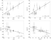 |
Fig. A.1. Same as Fig. 3 but for the common age scenario. The respective binary common age RM and IM solutions are detailed in Table A.1. |
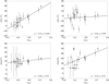 |
Fig. A.2. Same as Fig. 4 but for the common age scenario. The respective binary common age RM, IM, and CBM solutions are detailed in Table A.1. |
Same as Table 3 but with the equal age condition enforced.
All Tables
Summary of the grid of MESA stellar evolution models employed for the analysis of our sample stars.
All Figures
|
Fig. 1. Positions of individual binary components from our sample in Table 1 in the Teff − log g Kiel diagram. Blue squares and red triangles refer to the primary and secondary components, respectively. Evolutionary tracks are computed with solar metallicity Z = 0.014 and for an exponentially decaying CBM profile with fov = 0.02 Hp. Stellar mass is indicated in M⊙ units. |
| In the text | |
|
Fig. 2. Left: effect of the initial stellar mass M and of an exponentially decaying core-boundary mixing profile with parameter fov on evolutionary tracks. Mass (M = 10 (black), 12 (red), and 15 M⊙ (blue)) and mixing (fov = 0.005 (solid), 0.020 (dashed), and 0.040 Hp (dotted)) sequences are shown with color and line style, respectively. Solar metallicity Z = 0.014 is assumed. Right: effect of the initial stellar mass M and the metallicity Z on evolutionary tracks. The mass sequence is the same as in the left panel; line styles show the metallicity sequence Z = 0.010 (dashed), 0.014 (solid), and 0.018 (dotted) in mass fraction units. A fixed parameter fov = 0.005 Hp is assumed. Note the difference in X, Y-axes in the two panels. |
| In the text | |
|
Fig. 3. Stellar mass (top left), convective core mass (top right), and stellar age (bottom left) difference between the IM solution (cf. Sect. 4.3 and Table 3, column IM solution) and the RM solution (cf. Sect. 4.3 and Table 3, column RM solution) as a function of stellar surface gravity. The age difference as a function of the stellar mass difference between these two solutions is shown in the bottom right panel. All differences are expressed in percent relative to the RM solution values; the solid line depicts a linear fit in each of the four cases. The Spearman’s rank correlation coefficient (ρ) and the p-value of null hypothesis that there is no correlation between the two sets of variables are listed in each panel. |
| In the text | |
|
Fig. 4. Convective core mass (top row) and age (bottom row) changes due to the inclusion of extra near-core mixing in the models (cf. Table 3, column CBM solution). Left and right columns: comparisons against the RM solution (cf. Sect. 4.3 and Table 3, column RM solution) and the IM solution (cf. Sect. 4.3 and Table 3, column IM solution), respectively. |
| In the text | |
|
Fig. 5. Same as Fig. 4 but for the IM-CBM solution (cf. Sect. 4.3 and Table 3, column IM-CBM solution). Left and right columns: comparison against the IM (cf. Table 3, column IM solution) and CBM (cf. Table 3, column CBM solution) solutions, respectively. |
| In the text | |
|
Fig. 6. Left: remaining mass discrepancy after introducing an exponentially decaying CBM profile with radiative temperature gradient (the IM-CBM solution, cf. Sect. 4.3 and respective column in Table 3), defined as percentage of the dynamical mass of the star. Right: percentage difference between the mass discrepancy after (the IM-CBM solution) and before (the IM solution) the inclusion of CBM in the models. |
| In the text | |
|
Fig. 7. Relative change in the convective core mass (left) and age (right) of the star between solutions assuming a step-like and an exponentially decaying functional form of the CBM. The Y-axes are in percent relative to the value dictated by the solution with the exponentially decaying CBM. |
| In the text | |
|
Fig. 8. Left: temperature difference between a model atmosphere computed with a microturbulent velocity of ξ = 15 and 2 km s−1, as a function of the logarithm of the Rosseland optical depth. Right: differences in spectral line profiles associated with the change of microturbulent velocity in the model atmosphere from ξ = 2 km s−1 (solid black line) to ξ = 15 km s−1 (dashed red line). The difference spectrum (dotted blue line) was vertically shifted for clarity. Gaussian noise was added to both spectra to simulate a signal-to-noise ratio S/N ∼ 100. |
| In the text | |
|
Fig. 9. Left: four solutions obtained for the V380 Cyg system and detailed in Table 3. The corresponding MESA evolutionary tracks are shown with solid (dashed) lines for the primary (secondary) component. The RM, IM, CBM, and IM-CBM solutions are shown in black, red, blue, and green, respectively. The more (less) evolved primary (secondary) is shown with filled square (triangle) symbols. Right: changing position of the primary component (open square) associated with a reduced Teff by 8%. The color coding is the same as in the left panel. |
| In the text | |
|
Fig. 10. Convective core mass as a function of total mass for ZAMS models (full line) and models for the central hydrogen mass fractions of Xc = 0.35 (red) and Xc = 0.1 (black) when considering low (dashed), moderate (dashed-dot), and high (dotted) levels of CBM according to the ranges in Table 2. The sample stars are added with color coding according to their veq/vcirt (left) and their Xc (right). |
| In the text | |
|
Fig. A.1. Same as Fig. 3 but for the common age scenario. The respective binary common age RM and IM solutions are detailed in Table A.1. |
| In the text | |
|
Fig. A.2. Same as Fig. 4 but for the common age scenario. The respective binary common age RM, IM, and CBM solutions are detailed in Table A.1. |
| In the text | |
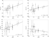 |
Fig. A.3. Same as Fig. 5 but with the equal age condition enforced. |
| In the text | |
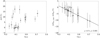 |
Fig. A.4. Same as Fig. 6 but with the equal age condition enforced. |
| In the text | |
Current usage metrics show cumulative count of Article Views (full-text article views including HTML views, PDF and ePub downloads, according to the available data) and Abstracts Views on Vision4Press platform.
Data correspond to usage on the plateform after 2015. The current usage metrics is available 48-96 hours after online publication and is updated daily on week days.
Initial download of the metrics may take a while.