| Issue |
A&A
Volume 636, April 2020
|
|
|---|---|---|
| Article Number | A10 | |
| Number of page(s) | 14 | |
| Section | Galactic structure, stellar clusters and populations | |
| DOI | https://doi.org/10.1051/0004-6361/202037688 | |
| Published online | 06 April 2020 | |
The effect of the environment-dependent IMF on the formation and metallicities of stars over the cosmic history
1
Department of Astrophysics/IMAPP, Radboud University, PO Box 9010, 6500 GL Nijmegen, The Netherlands
e-mail: This email address is being protected from spambots. You need JavaScript enabled to view it.
2
Helmholtz-Institut für Strahlen- und Kernphysik (HISKP), Universität Bonn, Nussallee 14–16, 53115 Bonn, Germany
e-mail: This email address is being protected from spambots. You need JavaScript enabled to view it.
3
Charles University in Prague, Faculty of Mathematics and Physics, Astronomical Institute, V Holešovičkách 2, 180 00 Praha 8, Czech Republic
4
Astronomical Institute, Czech Academy of Sciences, Fričova 298, 25165 Ondřejov, Czech Republic
5
Instituto de Astrofísica de Canarias, 38205 La Laguna, Tenerife, Spain
6
GRANTECAN, Cuesta de San Jose s/n, 38712 Breña Baja, La Palma, Spain
e-mail: This email address is being protected from spambots. You need JavaScript enabled to view it.
7
Institute for Astronomy, KU Leuven, Celestijnenlaan 200D, 3001 Leuven, Belgium
8
SRON, Netherlands Institute for Space Research, Sorbonnelaan 2, 3584 CA Utrecht, The Netherlands
Received:
7
February
2020
Accepted:
22
February
2020
Abstract
Recent observational and theoretical studies indicate that the stellar initial mass function (IMF) varies systematically with the environment (star formation rate – SFR, metallicity). Although the exact dependence of the IMF on those properties is likely to change with improving observational constraints, the reported trend in the shape of the IMF appears robust. We present the first study aiming to evaluate the effect of the IMF variations on the measured cosmic SFR density (SFRD) as a function of metallicity and redshift, fSFR(Z, z). We also study the expected number and metallicity of white dwarf, neutron star, and black hole progenitors under different IMF assumptions. Applying the empirically driven IMF variations described by the integrated galactic IMF (IGIMF) theory, we revise fSFR(Z, z) obtained in our previous study that assumed a universal IMF. We find a lower SFRD at high redshifts and a higher fraction of metal-poor stars being formed than previously determined. In the local Universe, our calculation applying the IGIMF theory suggests more white dwarf and neutron star progenitors in comparison with the universal IMF scenario, while the number of black hole progenitors remains unaffected.
Key words: galaxies: abundances / galaxies: stellar content / galaxies: star formation / stars: abundances / stars: formation
© ESO 2020
1. Introduction
The distribution of the cosmic star formation rate density (SFRD) at different metallicities and redshifts, fSFR(Z, z), is a necessary ingredient to estimate the rate of occurrence of any stellar or binary-evolution-related phenomenon. Among those, double compact object mergers and long gamma ray bursts are particularly sensitive to metallicity and their inferred rates, and the properties of their progenitor systems can vary significantly depending on the assumed fSFR(Z, z) (e.g. Chruslinska et al. 2019; Neijssel et al. 2019). Understanding the uncertainty of this distribution may be crucial to correctly comparing the theoretical estimates of the properties of those objects with observations and to exploring the physics behind the formation and evolution of their progenitors.
Recently, Chruslinska & Nelemans (2019; hereafter ChN19) tried to elucidate the observation-based fSFR(Z, z) distribution and to evaluate its uncertainty due to the currently unresolved issues involved in the observation of star forming galaxies. These issues include the unknown source of differences between the metallicity estimates obtained with different calibrations (e.g. Maiolino & Mannucci 2019), the poorly constrained low-mass end of the galaxy stellar mass function (e.g. Conselice et al. 2016), and the shape of the high-mass end of the star formation–mass relation (SFMR; some studies report a flattening of the high-mass part of the relation, e.g. Whitaker et al. 2014; Lee et al. 2015; Tomczak et al. 2016, while others find no evidence for such a flattening, e.g. Speagle et al. 2014; Pearson et al. 2018).
Chruslinska & Nelemans (2019) assume a universal Kroupa (2001) initial mass function (IMF) but note that the systematic variations in the IMF with the star formation rate (SFR) and/or metallicity (Z) may have a significant and non-straightforward impact on their results. However, the uncertainty of fSFR(Z, z) coming from this assumption could not be evaluated.
In fact, systematic variations of the IMF are expected on theoretical grounds (Larson 1998; Adams & Fatuzzo 1996; Adams & Laughlin 1996; Dib et al. 2007; Papadopoulos 2010) and have now been reported in many observational studies (see e.g. reviews by Kroupa et al. 2013; Hopkins 2018). There are observational indications of a top-heavy IMF in low-metallicity and high gas-density or high star-formation rate systems (e.g. Matteucci 1994; Dabringhausen et al. 2009, 2012; Papadopoulos 2010; Marks et al. 2012; Zhang et al. 2018; Brown & Wilson 2019; Kalari et al. 2018; Schneider et al. 2018), a top-light IMF in low star-formation rate systems (e.g. Lee et al. 2009; Meurer et al. 2009; Watts et al. 2018), and a bottom-heavy IMF in metal-rich environments (e.g. Kroupa 2002; Marks et al. 2012; Conroy et al. 2017; Martín-Navarro et al. 2015). A time-variable IMF that changes with evolving environmental properties is needed in order to explain all observational constraints (e.g. low-mass spectral features and chemical abundances such as [Mg/Fe], e.g. Vazdekis et al. 1997; Weidner et al. 2013a; Ferreras et al. 2015; Gargiulo et al. 2015; Fontanot et al. 2017; Jeřábková et al. 2018). A promising method to model the IMF variations, building on the integrated galactic IMF theory (IGIMF) put forward by Kroupa & Weidner (2003), has recently been developed by Yan et al. (2017, 2019b) and Jeřábková et al. (2018).
Here, we aim to evaluate the possible impact of the SFR- and metallicity-dependent IMF on the fSFR(Z, z). We combine the method described in ChN19 with the IGIMF, using the SFR and metallicity-dependent IMF model from Jeřábková et al. (2018). Our approach is summarised in Sect. 2. Our results are shown in Sect. 3; we focus on the differences between the fSFR(Z, z) obtained in this study and the distributions found in ChN19.
In general, the effect of the transition from a universal to a non-universal IMF will be different for stars forming in different mass ranges. Therefore, we also discuss the implications of the employed non-universal IMF model for the expected number and metallicity of stars forming in different mass ranges across cosmic history. This is important for the interpretation (in the case of observations) or estimation (in the case of theoretical studies) of the properties of populations of stars and objects composed of stars and their remnants. The choice of IMF model also affects the expected occurrence rates of various stellar evolution-related phenomena, because the formation efficiency of many transients of stellar or binary origin (e.g. double black hole mergers and long gamma ray bursts) depends on metallicity. Our results can provide guidance on whether the properties of stellar populations inferred under the assumption of the universal IMF may lead to over- or under-predictions of the estimated quantities and on the order of magnitude of this effect. The results of our calculations are available1.
Where appropriate we adopt a standard flat cosmology with ΩM = 0.3, ΩΛ = 0.7, and H0 = 70 km s−1 Mpc−1. All mentions of the universal or canonical IMF throughout this study refer to the Kroupa (2001, hereafter K01) IMF between 0.08 and 120 solar masses (M⊙).
2. Method
To estimate fSFR(Z, z) under the assumption of an evolving SFR- and metallicity-dependent IMF we combine the methods detailed in ChN19 and Jeřábková et al. (2018). Below we focus on the information relevant to this study and refer the reader to the original papers for further details.
2.1. Distribution of the cosmic SFR at different metallicities and redshifts
ChN19 construct the fSFR(Z, z) based on the empirical scaling relations for star forming galaxies combined over a wide range of redshifts and stellar masses of galaxies (Mgal,*). The observed galaxy stellar mass function (GSMF) of star forming galaxies is used to obtain the number density of objects of different masses. The metallicity (oxygen abundance) is then assigned to each mass with the use of the gas-based mass–metallicity relation (MZR). The star-formation–mass relation (SFMR) sets the contribution of galaxies of different masses (metallicities) to the total SFRD at a certain redshift. Combining them, one can obtain the fSFR(Z, z). The intrinsic scatter present in the relations, the internal distribution of metallicities in the star-forming gas within galaxies, and the so-called fundamental metallicity relation (i.e. the empirical relation between the Mgal,*, metallicity, and SFR of galaxies, which shows that galaxies of the same Mgal,* that have higher-than-average SFR simultaneously have lower-than-average metallicities, e.g. Mannucci et al. 2010) are taken into account. The above-mentioned empirical relations, as well as the results shown in ChN19 obtained with the use of those relations, assume the universal IMF.
2.2. The environment-dependent galaxy-wide IMF
To model the non-universal, environment-dependent IMF we rely on the description provided by the IGIMF theory (Weidner et al. 2013b; Yan et al. 2017; Jeřábková et al. 2018).
The IGIMF uses empirically derived prescriptions for the formation of stars on parsec and embedded cluster scales to build up galaxy-wide stellar populations. Those prescriptions are based on a few key inferences from the observations of the local star forming environments: (i) all stars form in embedded star clusters (Jeřábková et al. 2018; Lada & Lada 2003; Kroupa 2005; Megeath et al. 2016; Joncour et al. 2018); (ii) the IMF of each embedded star cluster varies with the gas density and metallicity of the star forming material in the cluster (i.e. the IMF becomes more top heavy in high gas-density and low-metallicity environments, e.g. Kroupa 2002; Dabringhausen et al. 2009; Marks et al. 2012) and is well approximated by a broken power law2; (iii) initial masses of star clusters are distributed according to a single power law, and the slope and the upper mass limit of the distribution depend on the SFR of a galaxy.
Star clusters with the same mass, metallicity, and density are assumed to lead to the same cluster IMF independent of their redshift. The galaxy-wide IMF and stellar population is then obtained by summing the contributions from the local galactic star-forming regions in a given time interval.
The IGIMF theory is consistent with the Milky Way stellar population and the galaxy-wide IMF. This is an important consistency check, since it is not clear a priori whether or not adding all the IMFs in all embedded clusters would yield a galaxy-wide IMF that agrees with the observational constraints (Mor et al. 2019; Zonoozi et al. 2019). The description of star formation with similar conditions as found in the present-day Milky Way is described robustly. Empirical relations describing conditions departing from well-measured regions in the Milky Way neighbourhood require improved measurements to be obtained, possibly with future instruments. Nevertheless, while the exact shape of the galaxy-wide IMF might change with an improved empirical description of star-formation, the expected trend of the IMF becoming top-heavy or top-light at high or low SFR, respectively, is now supported by a large variety of observations (e.g. Zhang et al. 2018; Brown & Wilson 2019; Kalari et al. 2018; Schneider et al. 2018; Lee et al. 2009; Watts et al. 2018; Conroy et al. 2017; Martín-Navarro et al. 2015).
In this study, we use the IGIMF3 model from Jeřábková et al. (2018), which implements the variation of the stellar IMF over the entire stellar mass range (see Fig. 1). We refer to the galaxy-wide IMF as described by the IGIMF3 model as the non-universal or environment-dependent IMF throughout the remainder of this paper. In Appendix B, we briefly discuss the difference in the results obtained with the IGIMF2 model from Jeřábková et al. (2018), which implements only variation of the high-mass part of the stellar IMF.
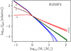 |
Fig. 1. Galaxy-wide IMFs computed using IGIMF3 as a function of stellar mass plotted for several values of SFR (10−3 – blue, 1.0 – green, 103 – red M⊙ yr−1) and [Fe/H] (−3, 0 2). The galaxy-wide IMFs are normalised by their values at 1 M⊙ to show the slope changes. The universal K01 IMF is plotted as a black dashed line. |
2.3. Star formation rate corrections for the non-universal IMF
The effect of a non-universal IMF on the fSFR(Z, z) can be estimated by determining the error associated with the observation-based galaxy SFR when assuming a universal IMF and then correcting for it. The observational estimates of the SFR rely on various tracers that typically measure the number of recently formed massive stars (e.g. UV luminosity, either measured directly or in the infrared when reprocessed by dust, and Hα emission from the recombination of gas ionised by the most massive stars; Madau & Dickinson 2014). This number can be converted to the total amount of mass turned into stars assuming a particular IMF (e.g. Kennicutt 1998; Kennicutt & Evans 2012; Madau & Dickinson 2014).
For a given SFR tracer, one can calculate the correction factor 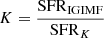 that allows to convert SFRK, the SFR estimate that assumes a universal IMF, to SFRIGIMF, the SFR that would be measured with a non-universal IMF(SFR, [Fe/H]3).
Chruslinska & Nelemans (2019) construct their SFMR using the relation found by Boogaard et al. (2018) for the local low-to-intermediate-mass galaxies and exploring three variations of the shape of the uncertain high-mass end of the relation (either a single power law, a broken power law, or a power law with a sharp flattening; see Fig. 5 in ChN19). This local relation, which sets the initial normalisation of the SFMR, relies on the Hα-based SFR measurements (i.e. the authors employ the Kennicutt 1998 relation). Therefore, we use the metallicity-dependent corrections to the Hα-based SFR to estimate the effect of the non-universal IMF on the fSFR(Z, z)4.
Such corrections to the Kennicutt (1998) relation were recently calculated by Jeřábková et al. (2018). Using the PyPegase python wrapper5, Jeřábková et al. (2018) combined the GalIMF code (Yan et al. 2017, 2019a) which computes the galaxy-wide IMF(SFR, [Fe/H]) with PEGASE.2 stellar population synthesis code (Fioc & Rocca-Volmerange 1999; Fioc et al. 2011) to produce the Hα flux for a given stellar population assuming a constant star formation history (SFH).
For the purpose of this paper we extended previous calculations for a larger parameter space of SFRs (10−5 M⊙ yr−1, 103 M⊙ yr−1) and [Fe/H] metallicities (−5, 1).
The corresponding relation between the universal IMF-based SFR and the SFR correction factor for the underlying non-universal IMF is shown in Fig. 2 for different [Fe/H] values.
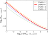 |
Fig. 2. Star formation rate estimated assuming the universal Kroupa (2001) IMF (SFRK01) and the corresponding correction factors (KK01 − IGIMF3) used to correct that SFR for the environment-dependent IMF (described by the IGIMF3 model from Jeřábková et al. 2018). Different lines show the dependence of the correction factor on metallicity (represented by [Fe/H]). For example, at log10(SFRK01) = −2 and [Fe/H] = −1, SFRIGIMF3 ≈ 100.6 SFRK01. |
The metallicity dependence of the IMF in Jeřábková et al. (2018) is parametrised using the relative iron abundance (relative to solar; [Fe/H]), while the observations used in ChN19 provide the oxygen abundance ZO/H (ZO/H = 12 + log10(O/H)). To combine the two methods, one needs to convert one metallicity measure to the other, which is not a straightforward procedure. However, we note that the metallicity dependence of the IMF has only a secondary effect on the correction factors calculated by Jeřábková et al. (2018) and so the exact form of the relation does not have a strong effect on our results. For the purpose of this study we assume an example relation between [O/H] and [Fe/H] as shown in Fig. 3 that takes into account the overabundance of oxygen with respect to iron relative to solar abundances at low metallicities (e.g. Wheeler et al. 1989; Zhang & Zhao 2005; Izotov et al. 2006; Tolstoy et al. 2009, see Appendix A for more details).
 |
Fig. 3. Assumed ZO/H – [Fe/H] conversion. The blue line results from Eqs. (A.1) and (A.2). We introduce normally distributed scatter (σ = 0.15 dex) around the central relation, indicated by the shaded area (showing 1σ distance from the line). The [Fe/H] = [O/H] relation is shown as the thick orange solid line for reference. The orange dashed lines indicate the solar metallicity in both measures. The black dashed lines roughly indicate the range of [Fe/H] probed in Milky Way studies (see Appendix A). |
Throughout this paper we use solar metallicity ZO/H⊙ = 8.83 as reported in Anders & Grevesse (1989), falling roughly in the middle of the range of the presently considered values (e.g. Delahaye & Pinsonneault 2006; Asplund et al. 2009; Vagnozzi et al. 2017).
2.4. Combining the two methods
The procedure applied to account for a non-universal IMF can be summarised as follows:
-
As in ChN19, we use the GSMF to obtain the number density of galaxies of different Mgal,* (ngal,*). In general, Mgal,* estimates are affected by the change in the underlying IMF. However, Mgal,* is only used to connect the various properties of galaxies and is not explicitly used in our calculations. Even though the Mgal,* would be different in the non-universal and the universal IMF cases, it would correspond to the same number density of objects. We assume here that the shape of the GSMF does not change when we change the IMF. This may not be strictly true for any non-universal IMF, but it is a reasonable assumption for the IMF variations considered in this study6.
-
As in ChN19, we assign the SFR to a certain ngal,* (via Mgal,* and GSMF) using the SFMR with scatter. The SFR estimate is affected by the change in the underlying IMF. We correct for this at a later step.
-
We assign the metallicity ZO/H to a certain ngal,* (via Mgal,* and GSMF) with the MZR, taking into account the scatter and the fundamental metallicity relation as described in ChN19. We assume that ZO/H estimates obtained for various metallicity calibrations are not significantly affected by the assumed IMF, i.e. if the underlying IMF is different from the assumed universal IMF, one would measure the same ZO/H.
-
We convert ZO/H to [Fe/H] as discussed in Sect. 2. This step is necessary, as the metallicity dependence of the IMF in Jeřábková et al. (2018) is parametrised using the iron abundance as a measure of metallicity.
-
Knowing the universal IMF-based SFR and [Fe/H] corresponding to a certain number density of galaxies, we calculate the correction factor for the SFR as described in Jeřábková et al. (2018) and estimate the corrected SFR.
-
We repeat the procedure at different redshifts, taking into account the evolution of the GSMF and the scaling relations, and construct the fSFR(Z, z).
3. Results
3.1. Effect on the fSFR(Z, z)
The general effect of the SFR corrections for the environment-dependent IMF is to increase the SFR of the low-mass galaxies and decrease that of the massive, highly star-forming galaxies. This means the galaxy main sequence is less steep and the total SFRD at a given redshift is less dominated by the contributions from the most massive, relatively metal-rich galaxies than expected under the assumption of an universal IMF.
This has two main effects on the fSFR(Z, z) distributions, as can be seen in Fig. 4, which shows a comparison of the effect of the change from the universal to non-universal IMF for two fSFR(Z, z) distributions: the high and low metallicity extremes introduced in ChN19. Those distributions were chosen as variations of the fSFR(Z, z) allowed by the current uncertainties in the empirical scaling relations that lead to the highest fraction of stellar mass that forms since z = 3 at high (>ZO/H⊙) and low (<0.1 ZO/H⊙) metallicity, respectively (see Appendix C for more details).
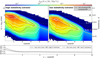 |
Fig. 4. Upper panels: distribution of the SFRD at different metallicities and redshifts (z). Left: background colour and brown contours show the high metallicity extreme assuming the non-universal IMF, and white contours show the high metallicity extreme assuming a universal IMF. Right: same as in the left panel, but for the low metallicity extreme. To plot the white contours, fSFR(Z, z) for the universal IMF cases has been re-scaled in such a way that the total SFRD at each redshift matches that of the corresponding variation with the non-universal IMF (see the bottom panel; the non-scaled fSFR(Z, z) in the universal IMF cases is shown in Fig. 8 in ChN19). This reveals the presence of the more extended low-metallicity tail present in the non-universal IMF variations. Bottom panel: ratio of the total SFRD at each redshift as calculated under the assumption of the non-universal to universal IMF for the two fSFR(Z, z) variations (dashed line – low-Z extreme, solid line – high-Z extreme). |
The first effect of changing to the non-universal IMF is the presence of a more pronounced low-metallicity tail in the fSFR(Z) distribution at any redshift, which can be seen by comparing the location of the white and brown contours in Fig. 4. Those contours show regions of the constant SFRD for several example values in the universal and non-universal IMF cases after eliminating the difference in the total SFRD (i.e. fSFR(Z, z) summed over metallicities at each redshift) between the two cases.
The second effect is on the total SFRD found at each redshift. The high-SFR end of the galaxy main sequence is the most strongly affected by the change in the underlying IMF, which results in a net reduction of the total SFRD at a given redshift when the non-universal IMF is assumed. This is demonstrated in the bottom panel of Fig. 4, which shows the ratio of the total SFRD at different z obtained under the assumption of the non-universal versus universal IMF. The ratio becomes more extreme towards higher redshifts because at relatively high SFRs the magnitude of the applied SFR corrections is larger and the average galactic SFR increases with z. There is also an additional trend with metallicity, causing the corrections at the high-SFR end to increase with decreasing metallicity (and therefore with increasing z, see Fig. 2).
3.2. Effect on the formation of stars of different masses
The assumption regarding the IMF also affects the distribution of the masses of stars forming with time as well as the distribution of metallicities at which those stars form.
The ratio of the number of stars formed in different mass ranges in the variable versus universal IMF case is shown in Fig. 5. Figure 6 demonstrates the corresponding ratio of the fraction of stars forming at low metallicity (below 10% ZO/H⊙) in different mass ranges. The ratios are shown for a few mass ranges that correspond to the conventionally adopted white dwarf (WD; M* < 8 M⊙), neutron star (NS; 8 M⊙ < M* < 20 M⊙), and black hole (BH; M* > 20 M⊙) progenitor mass limits7. We additionally separate the WD progenitor mass range below and above 1 M⊙8 and the mass range corresponding to the progenitors of the most massive stellar-origin BH i.e. stars of initial masses M* > 50 M⊙9. In general, the magnitude of the effect of the change in the IMF on the formation of stars in different mass ranges also depends on fSFR(Z, z). To demonstrate this, in Figs. 5 and 6 we show the ranges spanning between the ratios obtained using the limiting cases from ChN19, i.e. the low- (solid lines) and high-metallicity (dashed lines) extreme fSFR(Z, z) distributions. Before we zoom into the individual mass ranges, we discuss some general trends that appear in Figs. 5 and 6:
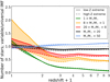 |
Fig. 5. Ratio of the number of stars forming in different mass ranges using the environment-dependent IMF to that using the universal IMF, as a function of redshift. The shaded area spans between the ratios obtained for the low- (solid lines) and high-metallicity (dashed lines) extreme fSFR(Z, z) distributions from ChN19. |
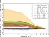 |
Fig. 6. Ratio of the fraction of stars forming at low metallicity (ZO/H < ZO/H⊙) in different mass ranges using the environment-dependent IMF to that using the universal IMF, as a function of redshift. The shaded area spans between the ratios obtained for the low- (solid lines) and high-metallicity (dashed lines) extreme fSFR(Z, z) distributions from ChN19. Thus, at redshift z = 1, about 2.5 times more stars with M* < 1 M⊙ form in the considered non-universal IMF scenario than in the universal IMF case. |
-
At high z the overall number of stars forming in the non-universal IMF scenario is smaller than in the universal IMF case.
-
The ratios in Fig. 5 increase towards lower z, and exceed unity at z < 1 if the fSFR(Z, z) distribution is similar to the low-Z extreme from ChN19.
-
The fraction of stars forming at low metallicity is increased in the non-universal IMF scenario. This fraction increases towards low z.
The above statements are common to all but the highest mass range (M* > 50 M⊙) considered, which shows the reverse behaviour. This is further discussed in Sect. 3.2.1. The trends seen in the remaining mass ranges can be understood by looking at Fig. 7. The thick light-grey curves in this figure show the SFR–metallicity relation at different redshifts as used in the high-Z extreme (top panel) and low-Z extreme (bottom panel) fSFR(Z, z) from ChN19. The coloured solid curves show that same relation after correcting the SFR for the non-universal IMF as discussed in Sect. 2.3. The colour shows the ratio of the number of stars formed in the NS progenitor mass range in the non-universal to universal IMF scenario in the different regions of the SFR–metallicity plane.
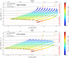 |
Fig. 7. Effect of the transition from the universal to environment-dependent IMF on the formation of the NS progenitors. The thick grey curves show the SFR–metallicity (ZO/H) relation as used in the high-Z extreme (top) and low-Z extreme (bottom) fSFR(Z, z) from ChN19 at different redshifts. The top metallicity axis ([Fe/H]) was obtained from ZO/H using the conversion described in Sect. 2. The coloured curves show the same relation after correcting the SFR for the non-universal IMF (see Fig. 2). The colour denotes the ratio of the number of stars forming in the NS progenitor mass range in the non-universal case to that in the universal IMF case. The near-horizontal grey lines are the lines of constant value of that ratio. The red dashed lines are the lines of the constant correction factor. The SFR below the thick red solid line is increased and above that line is decreased with respect to the universal IMF case. The vertical orange dashed lines show solar and 10% solar metallicity. |
It can be seen that at high redshifts the coloured curves fall almost entirely below the grey curves – i.e. the SFR of almost all galaxies is lowered with respect to the universal IMF case. This results in a decreased number of stars forming in the non-universal IMF scenario (but the strength of this effect differs for different masses of stars as shown in Fig. 5).
As the redshift decreases, the average SFR–metallicity relation shifts towards higher metallicities and lower SFR. This leads to higher positive SFR corrections at the low SFR side of the relation (see Fig. 2) and the increasing fraction of the low-SFR part of the coloured curves appears above the corresponding grey curves. At the same time, the decrease on the high-SFR end of the relation due to the correction is smaller. Hence, the ratio of the number of stars forming in the non-universal to the universal IMF scenario increases towards lower redshifts.
For the low-Z extreme fSFR(Z, z), almost the entire corrected relation at low z falls above the corresponding universal-IMF relation; i.e. the SFR of almost all galaxies is higher in the non-universal IMF scenario. In that case, the number of stars forming in different mass ranges exceeds that expected under the assumption of the universal IMF. In the high-Z extreme, the galaxies with the highest universal IMF SFRs receive negative corrections even at z ≈ 0 and hence the increase in the number of stars forming in the non-universal scenario when compared to those forming in the universal IMF scenario is smaller when this fSFR(Z, z) distribution is used.
The increase in the fraction of stars forming at low metallicity in the non-universal with respect to the universal IMF scenario is also readily seen in Fig. 7. The corrected SFR is always decreased on the high metallicity side and increased on the low metallicity side of the SFR–metallicity relation. The fractions shown in Fig. 6 correspond to metallicity below 10% solar and so at z > 8 (6) in the high-(low-) metallicity extreme, the ratio of the fractions of stars forming below that threshold is close to unity (nearly all star formation happens below 10% solar metallicity, i.e. to the left of the left-most orange vertical line in Fig. 7). The ratio then increases towards lower redshifts, as the SFR shifts to higher metallicities and is decreased above and increased below 0.1 ZO/H in the non-universal IMF scenario. The decrease at high ZO/H is stronger at higher z, while the increase at low ZO/H is stronger at lower z and the increase in the ratio starts to flatten between z = 1 and 2, where the two effects balance each other out. The ratio is smaller if the low-Z extreme fSFR(Z, z) is used, because in this case even at low redshifts a significant fraction of the total SFRD falls below 10% solar metallicity, irrespective of the assumptions regarding the IMF discussed in this study.
3.2.1. Black hole progenitors
The effect on the number and fraction of the most massive stars (BH progenitors) forming at low metallicity is shown by the black (stars with initial masses M* > 20 M⊙) and blue (M* > 50 M⊙) lines in Figs. 5 and 6, respectively. In general, this effect is very small. This is to be expected, as those stars, if present within a galaxy, are responsible for the emission of the bulk of the radiation that serves as an observable SFR tracer. In particular, the contribution to the Hα emission (considered as an SFR tracer in this study) comes only from the most massive stars (O and early-type B-stars with M* ≳ 17 M⊙, e.g. Madau & Dickinson 2014). This means that a stellar population forming according to a top-heavy IMF would have higher Hα luminosity per unit mass of star formed than that of a population forming according to the canonical MW-like IMF. Both IMFs can be used to interpret the measured luminosity as long as the inferred SFR is adjusted accordingly (i.e. it needs to be lower in the top-heavy IMF case). Therefore, the effects of the high-mass end slope of the IMF and the SFR counterbalance each other and the total number of the most massive stars formed and their metallicity distribution are not strongly affected by the IMF variations.
While the number of all stars more massive than 20 M⊙ forming at z ≳ 1 is slightly decreased, the number of those with the highest masses is higher in the non-universal IMF case. This is because the IMF is more top-heavy in the high-SFR and low-metallicity environments, which is typical of high-redshift galaxies, and the contribution to Hα luminosity increases with stellar mass. We find that formation of the massive (≳30 M⊙) stellar-origin BH from isolated stellar evolution in the low-redshift Universe is disfavoured. The progenitors of those BHs are believed to form at low metallicity with a mass of ≳50 M⊙. This is required to avoid strong stellar wind mass loss expected at high metallicities (e.g. Vink et al. 2001; Vink & de Koter 2005) and to retain enough mass during their evolution to form a massive remnant (e.g. Heger et al. 2003; Belczynski et al. 2010; Spera & Mapelli 2017). At low redshifts the star formation with such low metallicities happens predominantly in dwarf galaxies, forming stars at low rates ( ≲ 0.1 M⊙ yr−1). Those galaxies are deficient in massive stars as indicated by their Hα/UV emission (Pflamm-Altenburg et al. 2009; Lee et al. 2009; Meurer et al. 2009) and the photometry of resolved stellar populations (Watts et al. 2018). This is consistent with the prediction of the adopted IGIMF theory, which leads to the galaxy-wide IMF in the low-SFR (low mass) galaxies that is top-light and truncated at lower M* when compared to the universal IMF (see e.g. Fig. 1). Thus, those galaxies are less likely to be hosts of massive stellar-origin BHs.
3.2.2. Neutron star progenitors
The results for the stars forming with masses in the conventional NS progenitor mass range of 8–20 M⊙ follow the trends discussed earlier in this section and are indicated in red in Figs. 5 and 6. The number of stars forming in this mass range is lower in the non-universal IMF than in the universal IMF scenario, except for the low-redshift range of z ≲ 1 when the fSFR(Z, z) is described with the distribution similar to the low-Z extreme from ChN19. This decrease reaches a factor of about 1.3 at high z and is stronger than in the BH progenitors mass range, as the decrease in the SFR of the active galaxies due to the necessary corrections for the non-universal IMF is not fully counterbalanced by the change in the IMF in this mass range. The fraction of NS progenitors forming at low metallicity is increased by a factor of approximately 2 at low to intermediate redshifts if the non-universal IMF instead of the universal IMF is used.
3.2.3. White dwarf progenitors
The change from the universal to environment-dependent IMF has the strongest effect on the number and metallicity of the WD progenitors. We show this effect The number of WD progenitors and the fraction of those stars forming at low metallicity for the two IMF scenarios is shown in Figs. 5 and 6 respectively as orange (for initial masses 1–8 M⊙) and green (for M* < 1 M⊙) areas. The fraction of stars in the former mass range forming at low metallicity is up to a factor of approximately three to six higher (depending on the fSFR(Z, z)) at z ≲ 1.5 in the non-universal than in the universal-IMF scenario. The overall number of WD progenitors in the non-universal scenario with M* > 1 M⊙ is decreased with respect to the universal-IMF scenario by a factor of about two at z ≳ 1.5 and increased at low redshifts by up to a factor of two if the low-Z extreme fSFR(Z, z) is used. We discuss the importance of those effects for the formation of type Ia supernovae (SNIa) progenitors in Sect. 4.4.
The number of the lowest mass stars, that is, those of <1 M⊙, is decreased by more than a factor of ten at high z in the considered model of the IMF variations with respect to the universal IMF case. This is because the formation of low-mass stars is expected to be suppressed in the metal-poor and hot early Universe. This effect is expressed in the IGIMF formulation with a strong metallicity dependence of the low-mass part of the IMF, which is such that the IMF becomes increasingly bottom-light with decreasing metallicity (more relevant for the star formation at high redshifts) irrespective of the SFR (and vice versa in the environments with metallicities exceeding the solar value). The fraction of stars with M* < 1 M⊙ forming at low metallicity is still increased with respect to that expected in the universal IMF scenario due to a smaller reduction (at high z) or higher increase (at low z) in the SFR of the low-metallicity galaxies than in the SFR of the more metal-rich galaxies due to the applied corrections (see Fig. 2). We note that those two effects (i.e. decrease in the number of low-mass stars forming at high z and increase in the fraction of those forming at low metallicity at lower z) have the opposite effect on the metallicity distribution of all the low-mass stars ever formed. Therefore, this distribution is not significantly different between the considered universal and non-universal IMF scenarios. However, the age distribution of all the low-mass, low-metallicity stars ever formed that can still be observed in the local Universe would differ between the universal and non-universal IMF scenarios. In the latter case the bulk of the low-mass, low-metallicity stars form at later times in cosmic history and therefore their age distribution would be shifted to younger ages.
We note that the observational constraints on the metallicity dependence of the low-mass (<1 M⊙) end slope of the IMF are currently very limited (Kroupa 2002; Marks et al. 2012). If this dependence were found to be much weaker than assumed in the adopted IMF model, the results shown for the stars in this mass range would be closer to those shown for the more massive WD progenitors. This is shown in Appendix B, where we additionally discuss the difference in the results that would be obtained with no metallicity dependence of the low-mass part of the IMF (i.e. the IGIMF2 model from Jeřábková et al. 2018).
4. Discussion
The results presented here were obtained under the assumption of a particular parameterisation of the IMF dependence on SFR and metallicity. This description of the IMF variations has been validated mainly on the sample of relatively low-redshift galaxies (e.g. Yan et al. 2019b). We note that the exact form of this dependence is likely to be further elucidated with improving empirical constraints, especially at higher redshifts, but the expected trends in the shape of the IMF (e.g. top/bottom-heaviness at high/low SFR) with the environment are now reported in many observational studies and can therefore be assumed to be real.
Hence, our study should be treated as a qualitative discussion of the expected impact of the assumptions regarding the (non)universality of the IMF on the fSFR(Z, z) and the formation of stars in various mass ranges rather than a robust quantitative estimation of this effect. Our study provides guidance as to whether various calculations performed under the assumption of the universal IMF, e.g. estimates of the rates of different stellar-evolution-related phenomena (such as various types of SNe) are likely to under- or over-predict the estimated quantity and provides clues about the order of magnitude of this effect.
Besides being sensitive to the exact description of the IMF variations, our results are prone to uncertainties related to the calculations of the SFR correction factors, i.e. the conversion between the different metallicity measures, the stellar tracks used to perform the stellar population synthesis (in particular the uncertainties related to the treatment of the stellar winds, rotation, and binarity), and the adopted SFH of galaxies.
4.1. Metallicity conversion
In order to combine the IGIMF model with the fSFR(Z, z) from ChN19 and calculate the SFR correction factors, we need to convert ZO/H to the [Fe/H] metallicity measure. We achieve this by adopting a particular relation, as shown in Fig. 3. However, there is no universal way to translate the oxygen to iron abundance.
To demonstrate the impact of this assumption on our results, we additionally considered the simplest conversion [Fe/H] = [O/H] (represented by the thick orange line in Fig. 3, i.e. the iron abundance translates directly to oxygen abundance maintaining the solar ratios).
In that case, the estimated SFR of the low-metallicity, low-SFR galaxies would be higher than in the case where the conversion from Sect. 2 is applied. This is because the necessary SFR corrections for the variations in the underlying IMF are smaller at low metallicities and the effect of metallicity on the correction factor is more pronounced at low SFRs. The fraction of stars forming at low metallicity is therefore increased when the [Fe/H] = [O/H] conversion is used (see Fig. B.2). The overall effect is relatively small compared to that of the assumed fSFR(Z, z). The effect of the assumed metallicity conversion on the ratio of the number of stars forming in different mass ranges in the universal scenario to that in the non-universal IMF scenario is negligible (see Fig. B.3).
The realistic conversion would likely show some form of α-enhancement at low metallicities and high SFR and in this respect more closely resembles the conversion introduced in Sect. 2 rather than the simple [Fe/H] = [O/H] conversion (see Appendix A). We therefore conclude that this assumption does not have a significant effect on our results.
4.2. Stellar population synthesis
In order to estimate the Hα luminosity produced by a certain stellar population, one needs to model the stars that make up the population together with the light and spectra coming from their atmospheres. This is achieved with the use of stellar population synthesis (SPS) models (e.g. Leitherer et al. 1999; Fioc & Rocca-Volmerange 1999, 2019; Bruzual & Charlot 2003; Fioc et al. 2011). Different models differ in the implemented stellar and atmospheric models, but generally lead to comparable results (e.g. Jeřábková et al. 2017).
However, a number of effects (rotation, binary evolution) that are relevant for the modelling of the UV part of the spectrum are not taken into account in the commonly used SPS models, including the SPS model used in our analysis. These effects are also not taken into account in the observational studies estimating the galactic SFR used in ChN19. In general, taking into account the effects of binary evolution without including the effects of rotation has a similar effect on the modelled UV spectra to including the effects of rotation in single star models and not including the effects of binary evolution (Eldridge & Stanway 2009). Rotating stellar models show increased lifetimes, effective temperatures, and mass-loss rates when compared with the non-rotating ones (Ekström et al. 2012). In the case of binaries, interactions can for example remove the outer layers of stellar envelopes, rejuvenate the accreting star, or lead to the merger of two stars, with all these effects leading to increased emission in the blue part of the spectrum with respect to single models (e.g. Eldridge & Stanway 2009; Eldridge et al. 2017; Götberg et al. 2019). Both the effects of rotation and binarity increase the number of Wolf–Rayet stars and decrease the number of red supergiants present in the population (via increased mass-loss rates due to rotation or envelope stripping during mass transfer in binaries) and can increase the number of massive main sequence stars observed (rotation via extension of the lifetime by mixing more fuel into the core, binaries due to mass accretion; e.g. Eldridge & Stanway 2009).
Predicted spectral energy distributions tend to be “bluer” when the effect of binaries or rotation is considered and the corresponding stellar populations produce more UV/Hα flux for the same SFR with respect to those composed of single, non-rotating stars (leading to overestimated SFR based on those tracers). Götberg et al. (2019) find that the UV luminosity is not significantly affected by the presence of stars stripped of their envelopes in binary interactions in stellar populations in which star formation is ongoing or that are younger than about a few hundred millions years, but it may still be affected by the presence of other products of binary interaction. We note that the most rapid rotation is likely achieved in binaries (de Mink et al. 2013) and those effects have not been considered simultaneously. A more in-depth discussion of the effect of binary evolution and rotation on our results presents a challenge in itself and is beyond the scope of this study.
4.3. Assumption regarding the SFH
In order to compute SFR–Hα relations with the variable galaxy-wide IMF (and the SFR correction factors) we assume that the SFH is constant on timescales of >5 Myr (Jeřábková et al. 2018). This assumption ensures constant production of Hα by the stellar population. The Hα flux, being driven by the production of ionising photons, strongly depends on the population of massive stars (M* > 17 M⊙; we note that even though a 17 M⊙ star has a lifetime of a few tens of millions of years, the galactic Hα luminosity is dominated by the most massive stars with the shortest lifetimes) and thus consequently also on the SFH. For example, in the case of a single burst event, Hα flux values can differ by a few orders of magnitude in a few millions years when the most massive stars evolve. The assumption of constant SFH on timescales of several million years is therefore needed in order to provide any SFR–Hα relation (e.g. Kennicutt 1998; Pflamm-Altenburg et al. 2007, 2009).
The assumed SFH can be particularly important for the SFR estimates in galaxies with small values of SFR relative to the Milky Way. Those galaxies form only a very small number of high-mass (Hα producing), short-lived stars. Clearly, the estimated SFR will be different depending on whether the star is observed whilst alive or after it has completed its evolution. A proper evaluation of this effect is left to future studies; but see Pflamm-Altenburg et al. (2007) and Jeřábková et al. (2018) for further discussion of this problem.
4.4. Type Ia supernovae progenitors and supernovae rates
The greatest impact of the transition from the universal to the environment-dependent IMF is on the formation of stars in the WD progenitor mass range (e.g. Weidner & Kroupa 2005). A fraction of those stars are the progenitors of SNIa, which are believed to be thermonuclear explosions of relatively massive carbon-oxygen WDs. Two main SNIa formation channels are proposed, which have evolved over time. The first is the accretion model (evolved from the “single degenerate channel”) in which the explosion is triggered by accretion onto a WD, either by increasing the central density to ignition, or by triggering an explosion in the accreting layer that subsequently causes the accreting WD to explode. The second is the merger mode (evolved from the “double degenerate channel”) in which the explosion is triggered by the merger of two WDs. The explosion can be the result of the production of an unstable object that ignites due to a high temperature or density in some parts, or as a result of the merging itself and the shocks created in the process; see for example Maoz et al. (2014) and Livio & Mazzali (2018) for a detailed description of these models. Regardless of the exact formation scenario, the number of SNIa events expected from a certain stellar population depends on the IMF (see e.g. Sect. 4.5 in Yan et al. 2019b) and will be different in the universal and in the non-universal IMF scenarios. The assumptions regarding the IMF also affect the relative rates of different transients of stellar origin – we discuss SNIa and core collapse SNe (CCSNe) as an example below.
For illustrative purposes, here we follow the approach described in Yan et al. (2019b) and assume that the rate of SNeIa is proportional to the number of stars forming in the mass range suitable for the formation of the primary star in the SNIa progenitor system multiplied by the probability that a companion star also forms in the correct mass range. Both quantities are simply calculated from the IMF. We assume that the formation efficiency of SNeIa from progenitor binaries is constant and independent of the assumptions regarding the IMF. We are thus neglecting all the effects coming from the possible correlations between the initial binary parameters, binary evolution and metallicity. The dominant contribution of SNeIa in the commonly considered formation channels is found to come from progenitor stars with masses in the range ≈3–8 M⊙ (e.g. Claeys et al. 2014). Therefore, we assume that both stars in the type Ia progenitor binary come from this mass range. Analogous results to those shown in Figs. 5 and 6, but for the 3–8 M⊙ mass range of WD progenitors are shown in Appendix D. Furthermore, we assume that the delay time distribution follows a single power law ∝t−1, with a minimum time of 40 Myr as suggested by observations (Maoz & Mannucci 2012).
For CCSNe we simply assume that the rate is proportional to the number of stars forming in the mass range between 8 and 20 M⊙, again neglecting any metallicity or binary evolution-related effects (hence the ratio of the CCSN rate in the non-universal to universal IMF scenario is identical to the red range in Fig. 5).
The ratio of rates calculated under those assumptions in the non-universal to universal IMF scenario is shown in Fig. 8. Supernova rates to first approximation follow the SFR, and can therefore be expected to increase less steeply with z towards the peak of the SFH of the Universe in the non-universal scenario than in the universal IMF scenario (see e.g. Fig. C.1 for the cosmic SFH obtained for different IMF and fSFR(Z, z) assumptions used in this study). Except for the offset due to the longer delay time for SNIa explosions, their rate shows similar behaviour with redshift to CCSNe and so there is relatively little evolution with redshift in the ratio of SNIa to CCSN rate. The relative rate of SNeIa to that of CCSNe, as well as the rate of SNeIa as shown in Fig. 8, is lowered in the non-universal IMF scenario by a factor of a few, but we stress that the exact magnitude of this effect depends for example on the assumed delay time distribution of SNeIa. We note that the formation efficiency for SNeIa is not known theoretically but can be inferred from observations. Therefore, in order to explain the observed rate of SNeIa with a given progenitor model, this efficiency would simply need to be higher in the non-universal IMF scenario than in the universal IMF scenario. We note that at high z, that is, z ≳ 3, the presented trends are subject to additional uncertainty due to the uncertain contribution of dwarf galaxies to the cosmic SFRD (see Appendix C.1).
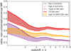 |
Fig. 8. Comparison of the results of the example calculation of the CCSN and SNIa rates as a function of redshift under different IMF assumptions. The hatched red area shows the ratio of the CCSN rate and the solid orange area shows the ratio of SNIa rate in the case with the non-universal IMF to that with the universal IMF. The dotted purple area shows the ratio of the relative rate of the SNIa to that of CCSN in the two IMF scenarios. The coloured areas span between the ratios obtained for calculations performed using the low- and high-metallicity extreme fSFR(Z, z) distributions. |
The above considerations neglect any potential metallicity effects on SNIa rates. However, the fraction of stars forming at low metallicity in the assumed SNIa progenitor mass range is increased by a factor of between approximately two and four (depending on the fSFR(Z, z) and IGIMF model; see Fig. D.1) at z ≲ 2 in the non-universal IMF scenario. This increase may be particularly important if the efficiency of formation of SNeIa depends on metallicity. In fact, some metallicity dependence has been reported in theoretical studies. For example, Toonen et al. (2012) find that the formation efficiency of SNeIa in the double degenerate channel can be up to 60% higher at low metallicity than at solar-like metallicities (these latter authors compare the models at solar and 5% solar metallicity). A potential correlation between the SNIa rate and galaxy metallicity has also been reported (e.g. Cooper et al. 2009, find an enhanced SNIa rate in star forming galaxies with lower metallicities). Such a correlation might be explained by the metallicity dependence of the IMF expected within the IGIMF theory.
5. Conclusions
In this study we evaluate the effect of the possible IMF variations on the distribution of the cosmic SFRD at different metallicities and redshifts. We also discuss the impact of those variations on the expected number and metallicity of WD, NS, and BH progenitors forming throughout cosmic history.
To this end, we use the empirically driven description of the SFR- and metallicity-dependent IMF based on IGIMF theory together with the SFR corrections from Jeřábková et al. (2018) and correct the observation-based fSFR(Z, z) from ChN19 for the underlying environment-dependent IMF.
While recent observational and theoretical studies indicate clear trends in the variation of the shape of the IMF with SFR and metallicity, the exact dependence of the IMF on the environment is likely to change with improving observational constraints. We therefore focus mainly on the qualitative effect of the applied corrections. Our main conclusions can be summarised as follows:
-
fSFR(Z, z) shows a more pronounced low-metallicity tail at all redshifts in the environment-dependent IMF scenario; the SFRD is less concentrated in the most massive, metal rich galaxies than in the universal-IMF case.
-
The total SFRD is decreased with respect to the universal IMF case at all but very low redshifts; the difference increases towards high redshifts and remains within a factor of approximately two for the considered IMF variation model.
-
Assuming the universal IMF may lead to underestimation of the fraction of NS and WD progenitors forming at low metallicity, especially at low redshifts. It may also lead to overestimation of the number of NS and WD progenitors forming at z ≳ 1 and an underestimation of the number of those stars forming at lower z. The strength of this effect depends on the fSFR(Z, z). The considered model for the IMF variations has the strongest effect on the number and metallicity of the WD progenitors with masses ≳1 M⊙, some of which are potential SNIa progenitors.
-
The transition from the universal IMF to the environment-dependent IMF has little effect on the formation of BH progenitors; the formation of the most massive BH progenitors at low metallicity in the local Universe is slightly disfavoured in the non-universal IMF scenario.
The results of our calculations are publicly available. They can be applied in studies aiming to estimate the properties of populations of stars and their remnants, stellar-evolution related transients and the environments in which they form. In particular, they can be used to gain insight into the effect of the IMF variations on the results of calculations that are typically performed under the assumption of the universal IMF.
We note that the IMF differs significantly from the canonical IMF mainly for extreme densities and very low metallicities.
[Fe/H] =  , where Fe and H stand for the number density of the corresponding atom.
We note that the normalisation of the SFMR relation in ChN19 is assumed to increases with redshift as found by Speagle et al. (2014) up to z = 1.8, and the rate of its evolution is adjusted to reproduce the observed flattening in the redshift evolution of SFMR normalisation at higher z (see Sect. 2.4 in ChN19 and references therein). Therefore, the SFMR constructed that way is not directly based on any particular tracer at higher z.
https://github.com/coljac/pypegase
We note that the updated version PEGASE.3 has recently been released (Fioc & Rocca-Volmerange 2019). The main difference with respect to PEGASE.2 is the addition of modelling of dust emission and its evolution, and the corresponding extent of computed wavelengths and therefore this does not affect the results shown in this study.
Construction of the GSMF involves binning the observed galaxies with respect to the inferred masses (which depend on the assumed IMF). One bin contains galaxies that have similar masses, but may differ in SFR and metallicity. Once the IMF becomes SFR- and metallicity-dependent, the galaxies in principle may “change bins”. However, the existence of the scaling relations guarantees that galaxies of similar masses have similar SFR and metallicity, and within the range of scatter the non-universal IMF as described by the IGIMF would not affect the masses within one bin in a very different way and so the shape of the GSMF would not be altered.
We note that those ranges are used for the convenience of discussion and for illustration purposes. The exact mass limits of the progenitors of different types of stellar remnants are uncertain and depend e.g. on metallicity, rotation, and the presence of binary interactions (e.g. Heger et al. 2003; Ekström et al. 2012; Ibeling & Heger 2013; Doherty et al. 2015). Particularly the boundary between BH and NS progenitors can differ significantly from the assumed limit and recent simulation results suggest that there may well not be a set mass boundary between them (e.g. Sukhbold & Woosley 2014; Sukhbold et al. 2016).
There are a few reasons for separating these mass ranges. 1 M⊙ is the conventional mass limit at which one of the IMF power law breaks occurs, separating the “high mass” from the “low mass” part of the IMF. Also, the difference between the IGIMF2 or IGIMF3 models from Jeřábková et al. (2018) lies in the description of the low-mass, i.e. <1 M⊙, part of the IMF (see Appendix B). Furthermore, stars forming below that mass have evolutionary timescales that are approaching the age of the Universe and therefore most of them have not turned into WD yet.
A ≈50 M⊙ star evolving in isolation at ≈10% solar metallicity is expected to leave behind a ≈20–40 M⊙ BH (e.g. Heger et al. 2003; Spera & Mapelli 2017; Mandel & Farmer 2018).
I.e., α1, 2 = αK01; 1, 2 + 0.5 [Fe/H], where α1 is the IMF slope between 0.08 and 0.5 M⊙ with αK01; 1 = 1.3 and α2 between 0.5 and 1 M⊙ with αK01; 2 = 2.3. The relation was derived between [Fe/H] of −2 dex to 0.2 dex and extrapolated outside this range.
Acknowledgments
We thank Søren Larsen and Jorryt Matthee for helpful discussions. We thank the organisers and the participants of the workshop “Metals in Galaxies, Near and Far: Looking Ahead” and the Lorentz Center for an inspiring workshop that encouraged this study. We thank the referee for their comments and a quick report. MC and GN acknowledge support from the Netherlands Organisation for Scientific Research (NWO). ZY acknowledges financial support from the China Scholarship Council (CSC, file number 201708080069). TJ acknowledges support by the Erasmus+ programme of the European Union under grant number 2017-1-CZ01- KA203-035562.
References
- Adams, F. C., & Fatuzzo, M. 1996, ApJ, 464, 256 [NASA ADS] [CrossRef] [Google Scholar]
- Adams, F. C., & Laughlin, G. 1996, ApJ, 468, 586 [NASA ADS] [CrossRef] [Google Scholar]
- Anders, E., & Grevesse, N. 1989, Geochim. Cosmochim. Acta, 53, 197 [Google Scholar]
- Asplund, M., Grevesse, N., Sauval, A. J., & Scott, P. 2009, ARA&A, 47, 481 [NASA ADS] [CrossRef] [Google Scholar]
- Belczynski, K., Bulik, T., Fryer, C. L., et al. 2010, ApJ, 714, 1217 [NASA ADS] [CrossRef] [Google Scholar]
- Bensby, T., Feltzing, S., & Lundström, I. 2004, A&A, 415, 155 [NASA ADS] [CrossRef] [EDP Sciences] [Google Scholar]
- Bensby, T., Feltzing, S., & Oey, M. S. 2014, A&A, 562, A71 [NASA ADS] [CrossRef] [EDP Sciences] [Google Scholar]
- Boogaard, L. A., Brinchmann, J., Bouché, N., et al. 2018, A&A, 619, A27 [NASA ADS] [CrossRef] [EDP Sciences] [Google Scholar]
- Bouwens, R. J., Illingworth, G. D., Oesch, P. A., et al. 2015, ApJ, 803, 34 [NASA ADS] [CrossRef] [Google Scholar]
- Brown, T., & Wilson, C. D. 2019, ApJ, 879, 17 [NASA ADS] [CrossRef] [Google Scholar]
- Bruzual, G., & Charlot, S. 2003, MNRAS, 344, 1000 [NASA ADS] [CrossRef] [Google Scholar]
- Chruslinska, M., & Nelemans, G. 2019, MNRAS, 488, 5300 [NASA ADS] [Google Scholar]
- Chruslinska, M., Nelemans, G., & Belczynski, K. 2019, MNRAS, 482, 5012 [NASA ADS] [CrossRef] [Google Scholar]
- Claeys, J. S. W., Pols, O. R., Izzard, R. G., Vink, J., & Verbunt, F. W. M. 2014, A&A, 563, A83 [NASA ADS] [CrossRef] [EDP Sciences] [Google Scholar]
- Conroy, C., van Dokkum, P. G., & Villaume, A. 2017, ApJ, 837, 166 [NASA ADS] [CrossRef] [Google Scholar]
- Conselice, C. J., Wilkinson, A., Duncan, K., & Mortlock, A. 2016, ApJ, 830, 83 [Google Scholar]
- Cooper, M. C., Newman, J. A., & Yan, R. 2009, ApJ, 704, 687 [NASA ADS] [CrossRef] [Google Scholar]
- Dabringhausen, J., Kroupa, P., & Baumgardt, H. 2009, MNRAS, 394, 1529 [NASA ADS] [CrossRef] [Google Scholar]
- Dabringhausen, J., Kroupa, P., Pflamm-Altenburg, J., & Mieske, S. 2012, ApJ, 747, 72 [NASA ADS] [CrossRef] [Google Scholar]
- de Mink, S. E., Langer, N., Izzard, R. G., Sana, H., & de Koter, A. 2013, ApJ, 764, 166 [NASA ADS] [CrossRef] [Google Scholar]
- Delahaye, F., & Pinsonneault, M. H. 2006, ApJ, 649, 529 [NASA ADS] [CrossRef] [Google Scholar]
- Dib, S., Kim, J., & Shadmehri, M. 2007, MNRAS, 381, L40 [NASA ADS] [CrossRef] [Google Scholar]
- Doherty, C. L., Gil-Pons, P., Siess, L., Lattanzio, J. C., & Lau, H. H. B. 2015, MNRAS, 446, 2599 [Google Scholar]
- Ekström, S., Georgy, C., Eggenberger, P., et al. 2012, A&A, 537, A146 [NASA ADS] [CrossRef] [EDP Sciences] [Google Scholar]
- Eldridge, J. J., & Stanway, E. R. 2009, MNRAS, 400, 1019 [NASA ADS] [CrossRef] [Google Scholar]
- Eldridge, J. J., Stanway, E. R., Xiao, L., et al. 2017, PASA, 34, e058 [NASA ADS] [CrossRef] [Google Scholar]
- Fermi-LAT Collaboration (Abdollahi, S., et al.) 2018, Science, 362, 1031 [NASA ADS] [CrossRef] [Google Scholar]
- Ferreras, I., Weidner, C., Vazdekis, A., & La Barbera, F. 2015, MNRAS, 448, L82 [NASA ADS] [CrossRef] [Google Scholar]
- Fioc, M., & Rocca-Volmerange, B. 1999, ArXiv e-prints [arXiv:astro-ph/9912179] [Google Scholar]
- Fioc, M., & Rocca-Volmerange, B. 2019, A&A, 623, A143 [NASA ADS] [CrossRef] [EDP Sciences] [Google Scholar]
- Fioc, M., Le Borgne, D., & Rocca-Volmerange, B. 2011, Astrophysics Source Code Library [record ascl:1108.007] [Google Scholar]
- Fontanot, F., De Lucia, G., Hirschmann, M., et al. 2017, MNRAS, 464, 3812 [NASA ADS] [CrossRef] [Google Scholar]
- Gargiulo, I. D., Cora, S. A., Padilla, N. D., et al. 2015, MNRAS, 446, 3820 [NASA ADS] [CrossRef] [Google Scholar]
- Götberg, Y., de Mink, S. E., Groh, J. H., Leitherer, C., & Norman, C. 2019, A&A, 629, A134 [NASA ADS] [CrossRef] [EDP Sciences] [Google Scholar]
- Heger, A., Fryer, C. L., Woosley, S. E., Langer, N., & Hartmann, D. H. 2003, ApJ, 591, 288 [NASA ADS] [CrossRef] [Google Scholar]
- Hopkins, A. M. 2018, PASA, 35, 39 [Google Scholar]
- Ibeling, D., & Heger, A. 2013, ApJ, 765, L43 [NASA ADS] [CrossRef] [Google Scholar]
- Izotov, Y. I., Stasińska, G., Meynet, G., Guseva, N. G., & Thuan, T. X. 2006, A&A, 448, 955 [NASA ADS] [CrossRef] [EDP Sciences] [Google Scholar]
- Jeřábková, T., Kroupa, P., Dabringhausen, J., Hilker, M., & Bekki, K. 2017, A&A, 608, A53 [NASA ADS] [CrossRef] [EDP Sciences] [Google Scholar]
- Jeřábková, T., Hasani Zonoozi, A., Kroupa, P., et al. 2018, A&A, 620, A39 [NASA ADS] [CrossRef] [EDP Sciences] [Google Scholar]
- Joncour, I., Duchêne, G., Moraux, E., & Motte, F. 2018, A&A, 620, A27 [NASA ADS] [CrossRef] [EDP Sciences] [Google Scholar]
- Kalari, V. M., Carraro, G., Evans, C. J., & Rubio, M. 2018, ApJ, 857, 132 [NASA ADS] [CrossRef] [Google Scholar]
- Kennicutt, R. C., Jr. 1998, ARA&A, 36, 189 [Google Scholar]
- Kennicutt, R. C., & Evans, N. J. 2012, ARA&A, 50, 531 [NASA ADS] [CrossRef] [Google Scholar]
- Kroupa, P. 2001, MNRAS, 322, 231 [NASA ADS] [CrossRef] [Google Scholar]
- Kroupa, P. 2002, Science, 295, 82 [NASA ADS] [CrossRef] [PubMed] [Google Scholar]
- Kroupa, P. 2005, in The Three-Dimensional Universe with Gaia, eds. C. Turon, K. S. O’Flaherty, & M. A. C. Perryman, ESA SP, 576, 629 [NASA ADS] [Google Scholar]
- Kroupa, P., & Weidner, C. 2003, ApJ, 598, 1076 [NASA ADS] [CrossRef] [Google Scholar]
- Kroupa, P., Weidner, C., Pflamm-Altenburg, J., et al. 2013, in The Stellar and Sub-Stellar Initial Mass Function of Simple and Composite Populations, eds. T. D. Oswalt, & G. Gilmore, 5, 115 [NASA ADS] [Google Scholar]
- Lada, C. J., & Lada, E. A. 2003, ARA&A, 41, 57 [NASA ADS] [CrossRef] [Google Scholar]
- Larson, R. B. 1998, MNRAS, 301, 569 [NASA ADS] [CrossRef] [Google Scholar]
- Lee, J. C., Gil de Paz, A., Tremonti, C., et al. 2009, ApJ, 706, 599 [NASA ADS] [CrossRef] [Google Scholar]
- Lee, N., Sanders, D. B., Casey, C. M., et al. 2015, ApJ, 801, 80 [NASA ADS] [CrossRef] [Google Scholar]
- Leitherer, C., Schaerer, D., Goldader, J. D., et al. 1999, ApJS, 123, 3 [NASA ADS] [CrossRef] [Google Scholar]
- Livio, M., & Mazzali, P. 2018, Phys. Rep., 736, 1 [NASA ADS] [CrossRef] [Google Scholar]
- Madau, P., & Dickinson, M. 2014, ARA&A, 52, 415 [NASA ADS] [CrossRef] [Google Scholar]
- Madau, P., & Fragos, T. 2017, ApJ, 840, 39 [NASA ADS] [CrossRef] [Google Scholar]
- Maiolino, R., & Mannucci, F. 2019, A&ARv, 27, 3 [NASA ADS] [CrossRef] [Google Scholar]
- Mandel, I., & Farmer, A. 2018, ArXiv e-prints [arXiv:1806.05820] [Google Scholar]
- Mannucci, F., Cresci, G., Maiolino, R., Marconi, A., & Gnerucci, A. 2010, MNRAS, 408, 2115 [NASA ADS] [CrossRef] [Google Scholar]
- Maoz, D., & Mannucci, F. 2012, PASA, 29, 447 [NASA ADS] [CrossRef] [Google Scholar]
- Maoz, D., Mannucci, F., & Nelemans, G. 2014, ARA&A, 52, 107 [NASA ADS] [CrossRef] [Google Scholar]
- Marks, M., Kroupa, P., Dabringhausen, J., & Pawlowski, M. S. 2012, MNRAS, 422, 2246 [NASA ADS] [CrossRef] [Google Scholar]
- Martín-Navarro, I., La Barbera, F., Vazdekis, A., Falcón-Barroso, J., & Ferreras, I. 2015, MNRAS, 447, 1033 [NASA ADS] [CrossRef] [Google Scholar]
- Matteucci, F. 1994, A&A, 288, 57 [NASA ADS] [Google Scholar]
- Megeath, S. T., Gutermuth, R., Muzerolle, J., et al. 2016, AJ, 151, 5 [NASA ADS] [CrossRef] [Google Scholar]
- Meurer, G. R., Wong, O. I., Kim, J. H., et al. 2009, ApJ, 695, 765 [NASA ADS] [CrossRef] [Google Scholar]
- Mor, R., Robin, A. C., Figueras, F., Roca-Fàbrega, S., & Luri, X. 2019, A&A, 624, L1 [NASA ADS] [CrossRef] [EDP Sciences] [Google Scholar]
- Neijssel, C. J., Vigna-Gómez, A., Stevenson, S., et al. 2019, MNRAS, 490, 3740 [NASA ADS] [CrossRef] [Google Scholar]
- Papadopoulos, P. P. 2010, ApJ, 720, 226 [NASA ADS] [CrossRef] [Google Scholar]
- Pearson, W. J., Wang, L., Hurley, P. D., et al. 2018, A&A, 615, A146 [NASA ADS] [CrossRef] [EDP Sciences] [Google Scholar]
- Pflamm-Altenburg, J., Weidner, C., & Kroupa, P. 2007, ApJ, 671, 1550 [NASA ADS] [CrossRef] [Google Scholar]
- Pflamm-Altenburg, J., Weidner, C., & Kroupa, P. 2009, MNRAS, 395, 394 [NASA ADS] [CrossRef] [Google Scholar]
- Reddy, B. E., Lambert, D. L., & Allende Prieto, C. 2006, MNRAS, 367, 1329 [NASA ADS] [CrossRef] [Google Scholar]
- Schneider, F. R. N., Ramírez-Agudelo, O. H., Tramper, F., et al. 2018, A&A, 618, A73 [NASA ADS] [CrossRef] [EDP Sciences] [Google Scholar]
- Speagle, J. S., Steinhardt, C. L., Capak, P. L., & Silverman, J. D. 2014, ApJS, 214, 15 [NASA ADS] [CrossRef] [Google Scholar]
- Spera, M., & Mapelli, M. 2017, MNRAS, 470, 4739 [Google Scholar]
- Steidel, C. C., Strom, A. L., Pettini, M., et al. 2016, ApJ, 826, 159 [NASA ADS] [CrossRef] [Google Scholar]
- Sukhbold, T., & Woosley, S. E. 2014, ApJ, 783, 10 [NASA ADS] [CrossRef] [Google Scholar]
- Sukhbold, T., Ertl, T., Woosley, S. E., Brown, J. M., & Janka, H. T. 2016, ApJ, 821, 38 [Google Scholar]
- Tolstoy, E., Hill, V., & Tosi, M. 2009, ARA&A, 47, 371 [NASA ADS] [CrossRef] [Google Scholar]
- Tomczak, A. R., Quadri, R. F., Tran, K.-V. H., et al. 2016, ApJ, 817, 118 [NASA ADS] [CrossRef] [Google Scholar]
- Toonen, S., Nelemans, G., & Portegies Zwart, S. 2012, A&A, 546, A70 [NASA ADS] [CrossRef] [EDP Sciences] [Google Scholar]
- Vagnozzi, S., Freese, K., & Zurbuchen, T. H. 2017, ApJ, 839, 55 [NASA ADS] [CrossRef] [Google Scholar]
- Vazdekis, A., Peletier, R. F., Beckman, J. E., & Casuso, E. 1997, ApJS, 111, 203 [NASA ADS] [CrossRef] [Google Scholar]
- Vink, J. S., & de Koter, A. 2005, A&A, 442, 587 [NASA ADS] [CrossRef] [EDP Sciences] [Google Scholar]
- Vink, J. S., de Koter, A., & Lamers, H. J. G. L. M. 2001, A&A, 369, 574 [NASA ADS] [CrossRef] [EDP Sciences] [Google Scholar]
- Watts, A. B., Meurer, G. R., Lagos, C. D. P., et al. 2018, MNRAS, 477, 5554 [NASA ADS] [CrossRef] [Google Scholar]
- Weidner, C., & Kroupa, P. 2005, ApJ, 625, 754 [NASA ADS] [CrossRef] [Google Scholar]
- Weidner, C., Ferreras, I., Vazdekis, A., & La Barbera, F. 2013a, MNRAS, 435, 2274 [NASA ADS] [CrossRef] [Google Scholar]
- Weidner, C., Kroupa, P., Pflamm-Altenburg, J., & Vazdekis, A. 2013b, MNRAS, 436, 3309 [NASA ADS] [CrossRef] [Google Scholar]
- Wheeler, J. C., Sneden, C., & Truran, J. W., Jr. 1989, ARA&A, 27, 279 [NASA ADS] [CrossRef] [Google Scholar]
- Whitaker, K. E., Franx, M., Leja, J., et al. 2014, ApJ, 795, 104 [NASA ADS] [CrossRef] [MathSciNet] [Google Scholar]
- Yan, Z., Jerabkova, T., & Kroupa, P. 2017, A&A, 607, A126 [NASA ADS] [CrossRef] [EDP Sciences] [Google Scholar]
- Yan, Z., Jerabkova, T., Kroupa, P., & Vazdekis, A. 2019a, A&A, 629, A93 [NASA ADS] [CrossRef] [EDP Sciences] [Google Scholar]
- Yan, Z., Jerabkova, T., & Kroupa, P. 2019b, Astrophysics Source Code Library [record ascl:1903.010] [Google Scholar]
- Zhang, H. W., & Zhao, G. 2005, MNRAS, 364, 712 [NASA ADS] [Google Scholar]
- Zhang, Z.-Y., Romano, D., Ivison, R. J., Papadopoulos, P. P., & Matteucci, F. 2018, Nature, 558, 260 [NASA ADS] [CrossRef] [Google Scholar]
- Zonoozi, A. H., Mahani, H., & Kroupa, P. 2019, MNRAS, 483, 46 [NASA ADS] [CrossRef] [Google Scholar]
Appendix A: Inferring iron abundances from the oxygen abundances
The simplest assumption to compare the ZO/H and [Fe/H] metallicity measurements would be that the [O/H] translates directly to [Fe/H] (maintaining the solar ratios; i.e. [O/H] = −1 translates to [Fe/H] = −1 etc.). However, this assumption may not be very realistic, as oxygen and iron are released to the interstellar medium on different timescales (e.g. Wheeler et al. 1989). While the former is abundantly produced by massive stars on timescales of millions of years, the latter is predominantly released in SNeIa that show a much longer (≈0.1–1 Gyr) delay with respect to the star formation episode. Therefore, young, low-metallicity star-forming systems are generally expected to be α-enhanced (i.e. show an overabundance of oxygen relative to iron with respect to solar, e.g. Zhang & Zhao 2005; Izotov et al. 2006). The difference in the timescales at which different elements are released to the interstellar medium is also reflected in the [O/Fe] versus [Fe/H] (or [O/H]) relation of a given stellar system: the oldest and the most metal-poor stellar populations (with [Fe/H] ≲ −1) are generally α-enhanced, with [O/Fe] approaching the ratio resulting from the core-collapse SN yields, but as the SNeIa start to release iron, the relation changes: [O/Fe] decreases and gradually reaches the solar-scaled values. However, the exact form of this relation (e.g. the location of the “knee” and the extreme [O/Fe] values) depends on the SFH and the IMF of a particular stellar system and is therefore not universal (e.g. Wheeler et al. 1989; Tolstoy et al. 2009). For the purpose of this study we assume an example relation between [O/Fe] and [Fe/H] that takes into account the overabundance of oxygen at low [Fe/H]:
![Mathematical equation: $$ \begin{aligned} \mathrm{[O/Fe]} = {\left\{ \begin{array}{ll} 0.5&\mathrm{if\, [Fe/H]} < -1 \\ -0.5 \times \mathrm{[Fe/H]}&\mathrm{if\, [Fe/H]}\ge -1, \end{array}\right.} \end{aligned} $$](/articles/aa/full_html/2020/04/aa37688-20/aa37688-20-eq3.gif) (A.1)
(A.1)
which is loosely guided by the Milky Way relation (e.g. Bensby et al. 2004, 2014; Reddy et al. 2006; Steidel et al. 2016). This relation is unconstrained at [Fe/H] > 0.2 but up to this point shows no evidence for flattening (as is seen for other α-elements, e.g. Bensby et al. 2004). We note that whether we assume that there is a flattening above [Fe/H] > 0.2 or extrapolate the relation from lower metallicities has no noticeable impact on our results. The conversion between ZO/H and [Fe/H] is then given by the relation:
![Mathematical equation: $$ \begin{aligned} \mathrm{[Fe/H]} = Z_{\mathrm{O/H}} - Z_{\mathrm{O/H} \odot } - \mathrm{[O/Fe]}, \end{aligned} $$](/articles/aa/full_html/2020/04/aa37688-20/aa37688-20-eq4.gif) (A.2)
(A.2)
where  is the solar oxygen abundance. The resulting ZO/H–[Fe/H] relation is shown in Fig. 3.
Appendix B: The impact of the IGIMF model and metallicity conversion
The difference between the IGIMF2 and IGIMF3 models from Jeřábková et al. (2018) lies mainly in the description of the low-mass part of the IMF (M* < 1M⊙); see Figs. B.1 and 1. In the IGIMF3 model the low-mass end of the IMF slope is assumed to follow the tentative empirical metallicity dependence described in Kroupa (2002) and Marks et al. (2012)10. In the IGIMF2 prescription the low-mass part of the IMF is fixed to the MW-like shape.
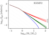 |
Fig. B.1. Galaxy-wide IMFs computed using IGIMF2 as a function of stellar mass plotted for several values of SFR (10−3, 1.0, 103 M⊙ yr−1) and metallicity (−3, 0 2). The galaxy-wide IMFs are normalised by their values for 1 M⊙ to show the slope changes. We note the main difference between the IGIMF2 and IGIMF3 (Fig. 1) models is the variation for the low-mass part of the galaxy-wide IMF. |
In the IGIMF3 prescription, the IMF is increasingly bottom-light at low metallicities, and so the formation efficiency of the low-mass stars (<1 M⊙) is decreased. The difference in the number of stars forming in this mass range in the IGIMF2 (IGIMF3) scenario with respect to the universal IMF reaches a factor of about 3 (≳10) at high redshifts (see Fig. B.3), where the increasing fraction of the star formation happens at low metallicity. When the IGIMF2 is used instead of the IGIMF3 description of the IMF variations, the increase in the fraction of low-mass stars forming at low metallicity with respect to the universal IMF case in the local Universe is enhanced by a factor of ≈1.5–2.5 (depending on the fSFR(Z, z) variation). This effect is the strongest for the high metallicity extreme and this case is shown in Fig. B.2. The shaded areas spanning between the solid and dashed lines in Fig. B.2 correspond to the fractions obtained using the IGIMF2 and IGIMF3 models respectively. It can be seen that the effect of the change between the two models on the results concerning more massive stars (>1 M⊙) is much smaller.
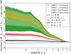 |
Fig. B.2. Ratio of the fraction of stars forming at low metallicity (ZO/H < 0.1 ZO/H⊙) in different mass ranges in the case with the environment-dependent IMF to that with the universal IMF as a function of redshift. The ratios are shown for the high metallicity extreme fSFR(Z, z) from Chruslinska & Nelemans (2019) and for two non-universal IMF models from Jeřábková et al. (2018): IGIMF2 model – solid line; IGIMF3 model – dashed line. The large shaded area between the solid and dashed lines spans between the ratios obtained for these two IMF models. The ratios are also mildly affected by the conversion of 12 + log10(O/H) to [Fe/H] metallicity measures. The thick solid and dashed curves were obtained for the default conversion described in Sect. 2. Using a conversion maintaining solar abundance ratios leads to a slight increase in the estimated ratios (thin lines, additional shadings). |
The effect of the choice of the IGIMF2/IGIMF3 model on the obtained cosmic SFH is negligible (see Fig. C.1). This choice also affects the global fSFR(Z, z) distribution (the fraction of stellar mass forming at low metallicity is increased in the IGIMF2 case with respect to the estimates based on the IGIMF3 model), but the effect is relatively small. To quantify the differences between the different fSFR(Z, z) versions, ChN19 compared the fraction of stellar mass that forms since z = 3 at low (<0.1 ZO/H⊙) and high (>ZO/H⊙) metallicity. We note that those quantities change by less than 2% between the fSFR(Z, z) obtained using IGIMF2 and IGIMF3 models (for a certain input universal IMF-based fSFR(Z, z)). For a fixed IMF model, that difference is at the level of 1% depending on the adopted metallicity conversion. For comparison, the low- and high-metallicity extremes are found to differ by 18% (22%) in terms of the low-metallicity mass fraction and by 26% (20%) in terms of the high-metallicity mass fraction for the universal (non-universal) IMF scenario.
The additional shaded areas above the thick solid and dashed lines in Figs. B.2 and B.3 indicate the fractions that would be obtained if ZO/H was assumed to translate to [Fe/H] maintaining the solar abundance ratios, instead of following the conversion described in Sect. 2. See Sect. 4.1 for further discussion.
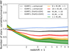 |
Fig. B.3. Ratio of the number of stars forming in different mass ranges in the case with the environment-dependent IMF to that with the universal IMF as a function of redshift. The ratios are shown for the high-metallicity extreme fSFR(Z, z) from Chruslinska & Nelemans (2019) and for two non-universal IMF models from Jeřábková et al. (2018): IGIMF2 model – solid line; IGIMF3 model – dashed line. The large shaded area between the solid and dashed lines spans between the ratios obtained for these two IMF models. The ratios are also mildly affected by the conversion of the 12 + log10(O/H) to [Fe/H] metallicity measures. The thick solid and dashed curves were obtained for the default conversion described in Sect. 2. Using conversion maintaining solar abundance ratios leads to slight increase in the estimated ratios (thin lines, additional shadings). |
Appendix C: The impact of the fSFR(Z, z)
The key difference between low- and high-Z extreme fSFR(Z, z) that is responsible for the differences in the ratios shown in Fig. 5 lies in the adopted SFR–(galaxy)mass relation. In the low-Z extreme the relation is assumed to flatten at high masses, and so the most massive galaxies have much lower SFRs than in the high-Z extreme (up to a factor of ≈100 for the highest masses, see Fig. 5 in ChN19). In the low redshift range this means that all galaxies in the low-Z extreme form stars at higher rates than expected in the universal IMF case (i.e. all receive positive corrections, see Fig. 2), and hence the number of stars forming in different mass ranges is generally higher in the non-universal than in the universal IMF case.
The SFR of the highly star forming galaxies in the high-Z extreme is decreased with respect to the universal IMF case even at low redshifts, which results in a smaller (or only slightly increased at low redshifts) number of stars forming in the non-universal IMF case with respect to the universal IMF scenario.
The difference in the metallicity description in the low- and high-Z extremes becomes important for the results shown in Fig. 5 only for the lowest considered mass range due to strong dependence of the low-mass part of the IMF on metallicity. In the adopted IMF variations model (IGIMF3 from Jeřábková et al. 2018 – this difference does not have a significant effect if the IGIMF2 model is used instead – see Appendix B), the formation of low-mass stars is favoured at high metallicities and this counteracts the effect of the SFR corrections in the metal rich, highly star forming galaxies on the formation of stars <1 M⊙, which leads to a relatively small difference in the ratios obtained for the low- and high-Z extremes in this mass range.
C.1. The discrepancy at high z reported in ChN19 and the non-universal IMF
The low and high metallicity extremes as discussed above and referred to throughout this paper were obtained in ChN19 under the assumption of a non-evolving low-mass end slope of the galaxy stellar mass function. As discussed in ChN19, there are some observational indications of the steepening trend of this slope with increasing redshift (see Sect. 3.1 therein). This leads to an increasing number density of the low-mass galaxies; hence the increasing contribution of the star formation at low metallicity to the total SFRD budget at high z.
This assumption has little effect on the results at z ≲ 3. However, it becomes important at higher z: if the slope of the low-mass end of the GSMF is allowed to steepen with redshift (and all the relations are simply extrapolated down to Mgal,* = 106 M⊙), the z ≳ 5 fSFR(Z, z) is completely dominated by the low-mass galaxies and low-metallicity star formation. ChN19 consider such variations of the fSFR(Z, z) at high z to be unrealistic, as they lead to flattening, or even a secondary peak at z ∼ 7 in the cosmic SFRD, instead of the observed decrease at z ≳ 2. This leads to significant overestimation of the total SFRD at these high redshifts with respect to other observational estimates of the cosmic SFRD (see Sects. 4.1.1 and 6.1).
As shown in Sect. 3, the SFRD at high z in the low- and high-Z extremes fSFR(Z, z) is lower in the non-universal IMF scenario than in the universal IMF scenario. However, the discrepancy reported in ChN19 in the fSFR(Z, z) cases with steepening low-mass end of the GSMF is due to the increasing contribution of the galaxies of the lowest masses and SFRs. The SFRs of those galaxies in the considered non-universal IMF scenario would be increased due to positive corrections even at high z (see Fig. 7). The lowered SFR of the more massive galaxies in the non-universal IMF scenario is not enough to compensate for that effect and the high-z SFRD still shows a peak at high z, which in the non-universal IMF scenario is higher than the peak at z ∼ 2. This is shown in Fig. C.1 for the high-Z extreme fSFR(Z, z)example.
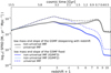 |
Fig. C.1. Cosmic SFH plotted for the universal (dashed lines) and non-universal (solid lines) IMF case using the high-Z extreme fSFR(Z, z) (thin lines) and the fSFR(Z, z) with the same MZR and SFMR, but with the slope of the low-mass end of the GSMF allowed to steepen with redshift as discussed in ChN19 (thick lines). For the high-Z extreme example we also show the cosmic SFH obtained using the IGIMF2 (light blue) or IGIMF3 (dark blue) non-universal IMF model. The former is slightly higher, but the difference is negligible. |
We note that the direct comparison of the results discussed in this study with the observational cosmic SFRD estimates (e.g. Madau & Dickinson 2014; Bouwens et al. 2015; Madau & Fragos 2017; Fermi-LAT Collaboration 2018) as done in ChN19 is no longer possible, as those estimates assume the universal IMF.
The assumption about the slope of the low-mass end of the GSMF would also affect the results shown in Figs. 5 and 6 at high redshifts. The fraction of the number of stars forming in the non-universal versus universal IMF scenario for different assumptions regarding the low-mass end of the GSMF in Fig. C.2. If the low-mass end of the GSMF steepens with redshift, the number of stars forming at z ≳ 3 in the massive WD, NS, and lower-mass BH progenitor mass range is increased in the non-universal with respect to universal IMF scenario. In that case, the star formation at high z happens predominantly in galaxies with low metallicity and SFR ≈ 0.1 M⊙ yr−1 that in the adopted non-universal IMF scenario have simultaneously bottom- and top-light IMFs, which favours the formation of stars in this mass range with respect to universal IMF. The main difference in the ratio of the fraction of stars forming at low metallicity in the non-universal versus universal IMF case due to the GSMF with the steepening slope would be an earlier decrease at z > 2 (as the fraction of stars forming at low Z approaches 1 at lower redshift in this GSMF variation).
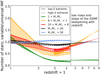 |
Fig. C.2. Same as Fig. 5, but with additional lines included to demonstrate the impact of the assumption regarding the slope of the low-mass end of the GSMF. At z ≲ 2 the ratio is not affected by this assumption. At z ≳ 3, the difference becomes apparent – if the slope of the low-mass end of the GSMF is fixed (as in the cases shown in Fig. 5), the trend flattens and the ratio remains at the level reached at z ∼ 3. If the slope steepens with redshift, the ratio for the stars in the intermediate-mass WD and NS progenitor mass range starts to increase with z. |
Appendix D: Zoom into the SNIa progenitor mass range
Figure D.1 shows the fraction of low-metallicity stars and the number of stars forming in the 3–8 M⊙ mass range in the non-universal and universal IMF scenarios. The additional shadings demonstrate the difference between the IGIMF2 and IGIMF3 (Fig. 7) non-universal IMF models.
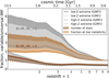 |
Fig. D.1. Ratio of the fraction of stars forming at low metallicity (ZO/H < ZO/H⊙) in the non-universal and universal IMF scenarios (hatched filled area) and the ratio of the number of stars forming in the two IMF scenarios (filled area), as a function of redshift. The solid lines correspond to low-Z extreme fSFR(Z, z) distributions and the dashed lines to high-Z extreme fSFR(Z, z) distributions. The thick lines correspond to the IGIMF3 model, while the thin lines show the IGIMF2 model (lower than the corresponding IGIMF3 lines). The coloured areas correspond to stars with initial masses in the range of 3–8 M⊙, which is the mass range relevant for the formation of the progenitors of SNeIa. The grey areas in the background correspond to the WD progenitors with initial masses in the range of 1–8 M⊙ (same as in Figs. 5 and 6). |
All Figures
|
Fig. 1. Galaxy-wide IMFs computed using IGIMF3 as a function of stellar mass plotted for several values of SFR (10−3 – blue, 1.0 – green, 103 – red M⊙ yr−1) and [Fe/H] (−3, 0 2). The galaxy-wide IMFs are normalised by their values at 1 M⊙ to show the slope changes. The universal K01 IMF is plotted as a black dashed line. |
| In the text | |
|
Fig. 2. Star formation rate estimated assuming the universal Kroupa (2001) IMF (SFRK01) and the corresponding correction factors (KK01 − IGIMF3) used to correct that SFR for the environment-dependent IMF (described by the IGIMF3 model from Jeřábková et al. 2018). Different lines show the dependence of the correction factor on metallicity (represented by [Fe/H]). For example, at log10(SFRK01) = −2 and [Fe/H] = −1, SFRIGIMF3 ≈ 100.6 SFRK01. |
| In the text | |
|
Fig. 3. Assumed ZO/H – [Fe/H] conversion. The blue line results from Eqs. (A.1) and (A.2). We introduce normally distributed scatter (σ = 0.15 dex) around the central relation, indicated by the shaded area (showing 1σ distance from the line). The [Fe/H] = [O/H] relation is shown as the thick orange solid line for reference. The orange dashed lines indicate the solar metallicity in both measures. The black dashed lines roughly indicate the range of [Fe/H] probed in Milky Way studies (see Appendix A). |
| In the text | |
|
Fig. 4. Upper panels: distribution of the SFRD at different metallicities and redshifts (z). Left: background colour and brown contours show the high metallicity extreme assuming the non-universal IMF, and white contours show the high metallicity extreme assuming a universal IMF. Right: same as in the left panel, but for the low metallicity extreme. To plot the white contours, fSFR(Z, z) for the universal IMF cases has been re-scaled in such a way that the total SFRD at each redshift matches that of the corresponding variation with the non-universal IMF (see the bottom panel; the non-scaled fSFR(Z, z) in the universal IMF cases is shown in Fig. 8 in ChN19). This reveals the presence of the more extended low-metallicity tail present in the non-universal IMF variations. Bottom panel: ratio of the total SFRD at each redshift as calculated under the assumption of the non-universal to universal IMF for the two fSFR(Z, z) variations (dashed line – low-Z extreme, solid line – high-Z extreme). |
| In the text | |
|
Fig. 5. Ratio of the number of stars forming in different mass ranges using the environment-dependent IMF to that using the universal IMF, as a function of redshift. The shaded area spans between the ratios obtained for the low- (solid lines) and high-metallicity (dashed lines) extreme fSFR(Z, z) distributions from ChN19. |
| In the text | |
|
Fig. 6. Ratio of the fraction of stars forming at low metallicity (ZO/H < ZO/H⊙) in different mass ranges using the environment-dependent IMF to that using the universal IMF, as a function of redshift. The shaded area spans between the ratios obtained for the low- (solid lines) and high-metallicity (dashed lines) extreme fSFR(Z, z) distributions from ChN19. Thus, at redshift z = 1, about 2.5 times more stars with M* < 1 M⊙ form in the considered non-universal IMF scenario than in the universal IMF case. |
| In the text | |
|
Fig. 7. Effect of the transition from the universal to environment-dependent IMF on the formation of the NS progenitors. The thick grey curves show the SFR–metallicity (ZO/H) relation as used in the high-Z extreme (top) and low-Z extreme (bottom) fSFR(Z, z) from ChN19 at different redshifts. The top metallicity axis ([Fe/H]) was obtained from ZO/H using the conversion described in Sect. 2. The coloured curves show the same relation after correcting the SFR for the non-universal IMF (see Fig. 2). The colour denotes the ratio of the number of stars forming in the NS progenitor mass range in the non-universal case to that in the universal IMF case. The near-horizontal grey lines are the lines of constant value of that ratio. The red dashed lines are the lines of the constant correction factor. The SFR below the thick red solid line is increased and above that line is decreased with respect to the universal IMF case. The vertical orange dashed lines show solar and 10% solar metallicity. |
| In the text | |
|
Fig. 8. Comparison of the results of the example calculation of the CCSN and SNIa rates as a function of redshift under different IMF assumptions. The hatched red area shows the ratio of the CCSN rate and the solid orange area shows the ratio of SNIa rate in the case with the non-universal IMF to that with the universal IMF. The dotted purple area shows the ratio of the relative rate of the SNIa to that of CCSN in the two IMF scenarios. The coloured areas span between the ratios obtained for calculations performed using the low- and high-metallicity extreme fSFR(Z, z) distributions. |
| In the text | |
|
Fig. B.1. Galaxy-wide IMFs computed using IGIMF2 as a function of stellar mass plotted for several values of SFR (10−3, 1.0, 103 M⊙ yr−1) and metallicity (−3, 0 2). The galaxy-wide IMFs are normalised by their values for 1 M⊙ to show the slope changes. We note the main difference between the IGIMF2 and IGIMF3 (Fig. 1) models is the variation for the low-mass part of the galaxy-wide IMF. |
| In the text | |
|
Fig. B.2. Ratio of the fraction of stars forming at low metallicity (ZO/H < 0.1 ZO/H⊙) in different mass ranges in the case with the environment-dependent IMF to that with the universal IMF as a function of redshift. The ratios are shown for the high metallicity extreme fSFR(Z, z) from Chruslinska & Nelemans (2019) and for two non-universal IMF models from Jeřábková et al. (2018): IGIMF2 model – solid line; IGIMF3 model – dashed line. The large shaded area between the solid and dashed lines spans between the ratios obtained for these two IMF models. The ratios are also mildly affected by the conversion of 12 + log10(O/H) to [Fe/H] metallicity measures. The thick solid and dashed curves were obtained for the default conversion described in Sect. 2. Using a conversion maintaining solar abundance ratios leads to a slight increase in the estimated ratios (thin lines, additional shadings). |
| In the text | |
|
Fig. B.3. Ratio of the number of stars forming in different mass ranges in the case with the environment-dependent IMF to that with the universal IMF as a function of redshift. The ratios are shown for the high-metallicity extreme fSFR(Z, z) from Chruslinska & Nelemans (2019) and for two non-universal IMF models from Jeřábková et al. (2018): IGIMF2 model – solid line; IGIMF3 model – dashed line. The large shaded area between the solid and dashed lines spans between the ratios obtained for these two IMF models. The ratios are also mildly affected by the conversion of the 12 + log10(O/H) to [Fe/H] metallicity measures. The thick solid and dashed curves were obtained for the default conversion described in Sect. 2. Using conversion maintaining solar abundance ratios leads to slight increase in the estimated ratios (thin lines, additional shadings). |
| In the text | |
|
Fig. C.1. Cosmic SFH plotted for the universal (dashed lines) and non-universal (solid lines) IMF case using the high-Z extreme fSFR(Z, z) (thin lines) and the fSFR(Z, z) with the same MZR and SFMR, but with the slope of the low-mass end of the GSMF allowed to steepen with redshift as discussed in ChN19 (thick lines). For the high-Z extreme example we also show the cosmic SFH obtained using the IGIMF2 (light blue) or IGIMF3 (dark blue) non-universal IMF model. The former is slightly higher, but the difference is negligible. |
| In the text | |
|
Fig. C.2. Same as Fig. 5, but with additional lines included to demonstrate the impact of the assumption regarding the slope of the low-mass end of the GSMF. At z ≲ 2 the ratio is not affected by this assumption. At z ≳ 3, the difference becomes apparent – if the slope of the low-mass end of the GSMF is fixed (as in the cases shown in Fig. 5), the trend flattens and the ratio remains at the level reached at z ∼ 3. If the slope steepens with redshift, the ratio for the stars in the intermediate-mass WD and NS progenitor mass range starts to increase with z. |
| In the text | |
|
Fig. D.1. Ratio of the fraction of stars forming at low metallicity (ZO/H < ZO/H⊙) in the non-universal and universal IMF scenarios (hatched filled area) and the ratio of the number of stars forming in the two IMF scenarios (filled area), as a function of redshift. The solid lines correspond to low-Z extreme fSFR(Z, z) distributions and the dashed lines to high-Z extreme fSFR(Z, z) distributions. The thick lines correspond to the IGIMF3 model, while the thin lines show the IGIMF2 model (lower than the corresponding IGIMF3 lines). The coloured areas correspond to stars with initial masses in the range of 3–8 M⊙, which is the mass range relevant for the formation of the progenitors of SNeIa. The grey areas in the background correspond to the WD progenitors with initial masses in the range of 1–8 M⊙ (same as in Figs. 5 and 6). |
| In the text | |
Current usage metrics show cumulative count of Article Views (full-text article views including HTML views, PDF and ePub downloads, according to the available data) and Abstracts Views on Vision4Press platform.
Data correspond to usage on the plateform after 2015. The current usage metrics is available 48-96 hours after online publication and is updated daily on week days.
Initial download of the metrics may take a while.