| Issue |
A&A
Volume 635, March 2020
|
|
|---|---|---|
| Article Number | A109 | |
| Number of page(s) | 6 | |
| Section | The Sun and the Heliosphere | |
| DOI | https://doi.org/10.1051/0004-6361/201937321 | |
| Published online | 17 March 2020 | |
Solar Rossby waves observed in GONG++ ring-diagram flow maps
1
Center for Space Science, NYUAD Institute, New York University Abu Dhabi, Abu Dhabi, UAE
e-mail: This email address is being protected from spambots. You need JavaScript enabled to view it.
2
Max-Planck-Institut für Sonnensystemforschung, Justus-von-Liebig-Weg 3, 37077 Göttingen, Germany
3
Institut für Astrophysik, Georg-August-Universität Göttingen, Friedrich-Hund-Platz 1, 37077 Göttingen, Germany
Received:
15
December
2019
Accepted:
31
January
2020
Abstract
Context. Solar Rossby waves have only recently been unambiguously identified in Helioseimsic and Magnetic Imager (HMI) and Michelson Doppler Imager maps of flows near the solar surface. So far this has not been done with the Global Oscillation Network Group (GONG) ground-based observations, which have different noise properties.
Aims. We use 17 years of GONG++ data to identify and characterize solar Rossby waves using ring-diagram helioseismology. We compare directly with HMI ring-diagram analysis.
Methods. Maps of the radial vorticity were obtained for flows within the top 2 Mm of the surface for 17 years of GONG++ data. The data were corrected for systematic effects including the annual periodicity related to the B0 angle. We then computed the Fourier components of the radial vorticity of the flows in the co-rotating frame. We performed the same analysis on the HMI data that overlap in time.
Results. We find that the solar Rossby waves have measurable amplitudes in the GONG++ sectoral power spectra for azimuthal orders between m = 3 and m = 15. The measured mode characteristics (frequencies, lifetimes, and amplitudes) from GONG++ are consistent with the HMI measurements in the overlap period from 2010 to 2018 for m ≤ 9. For higher-m modes the amplitudes and frequencies agree within two sigmas. The signal-to-noise ratio of modes in GONG++ power spectra is comparable to those of HMI for 8 ≤ m ≤ 11, but is lower by a factor of two for other modes.
Conclusions. The GONG++ data provide a long and uniform data set that can be used to study solar global-scale Rossby waves from 2001.
Key words: Sun: helioseismology / Sun: oscillations / Sun: interior / waves
© ESO 2020
1. Introduction
Löptien et al. (2018) recently discovered solar global-scale Rossby waves (or r modes) in the surface flow fields derived from observations by the Helioseismic and Magnetic Imager on board the Solar Dynamics Observatory (SDO/HMI, Scherrer et al. 2012; Schou et al. 2012). The Rossby waves are potentially important as they could be probes of the deep convection zone. Liang et al. (2019) confirmed this result using time-distance helioseismology applied to both SDO/HMI and Michelson Doppler Imager (MDI) observations on board the Solar and Heliospheric Observatory. It has yet to be seen how well the r modes show in the flow maps produced by the Global Oscillation Group Network pipeline (GONG++). This is the goal of this study.
In the first Rossby wave findings, Löptien et al. (2018) generated radial vorticity maps from flow maps measured by local correlation tracking (LCT) of granules (Welsch et al. 2004; Fisher et al. 2008) and ring-diagram analysis (RDA, Hill 1988). These authors found that the sectoral r-mode spectrum closely follows the standard theoretical dispersion relation ω = − 2Ωeq/(m + 1), where Ωeq/2π = 453.1 nHz is the equatorial rotation rate and m is the azimuthal order (see, e.g., Saio 1982). Liang et al. (2019) confirmed the results of Löptien et al. (2018) using time-distance helioseismology on the meridional component uy of the horizontal flow near the equator. Unlike Löptien et al. (2018), who imaged near-surface layers, Liang et al. (2019) imaged at a depth of 0.91 R⊙. These latter authors used 21 years of data spanning both the observation sets of MDI and HMI from 1996 to 2017. Meanwhile, Hanasoge & Mandal (2019) provided another independent means of detecting solar r modes, through the use of normal-mode coupling in two years of HMI data. Additionally, Proxauf et al. (2020) investigated the latitudinal and depth dependence of the r modes using HMI ring-diagram analysis. Finally, in an effort to assess the accuracy of machine-learning techniques for ring-diagram analysis, Alshehhi et al. (2019) used r modes as a litmus test on the suitability of this new technique for helioseismic inversions.
In this study we aim to contribute to this growing literature on solar Rossby waves, with an analysis of the 17 years of data from GONG++ and compare a subset of these data to the overlapping observations of HMI. Here, we focus on using the RDA products from both the GONG++ and HMI pipelines. The GONG++ data are interesting for solar r-mode characterization for two reasons. Firstly, the GONG data and HMI data overlap since 2010, enabling the direct comparison of two data sets produced by similar pipelines, but with different noise properties. Secondly, while Liang et al. (2019) merged the MDI (14 years) and HMI (7 years) data to create a combined 21 years of data, the GONG++ data should be uniform for 17 years. In this study we explore the signature of the solar r modes in the GONG++ data and report differences with the HMI data.
2. Data analysis and results
2.1. Ring-diagram analysis
We use ring-diagram flow maps generated by the GONG++ pipeline from September 2001 to February 2019. The pipeline follows the method outlined in Corbard et al. (2003), whereby flows are computed from the p-mode frequency shifts extracted from tracked patches (tiles) of the Doppler velocity. These patches are tracked across a transverse cylindrical equidistant projection of the solar disk for approximately 27 h, following the Snodgrass rotation profile (e.g., Eq. (3) of Corbard et al. 2003). For every day of tracking there are 189 tiles across the solar disk.
For each tile, the two horizontal components of the flows in the x (prograde) and y (northward) directions (ux, uy) are computed as follows: A 2D cosine bell apodization is applied to a 16° ×16° square patch in order to obtain a circular tile of radius 15°. For each data cube of the Doppler velocity Ψ(x, y, t), a 3D Fourier transform is performed to generate spectral cubes  , from which the power spectrum
  is computed. For each fixed wave number
  , a cylindrical cut through the power spectrum is made to generate 𝒫k(ϑ, ω), where ϑ is the angle between the wave vector and the prograde direction (Bogart et al. 1995). In the absence of flows, acoustic modes appear as horizontal ridges in 𝒫k(ϑ, ω). The presence of flows causes Doppler frequency shifts that depend on the magnitude and direction of flow. The observed ridges are fit with a six parameter Lorentzian-like model (e.g., Haber et al. 2000). For each p-mode radial order n and wave number k, two flow parameters (Ux, Uy) are extracted from the data. The physical flow (ux, uy) at a particular depth in the interior is inferred by inverting the set of measured parameters. In the current study we restrict our attention to the flows at a depth of 2 Mm.
2.2. Sectoral power spectra of radial vorticity
With the horizontal flow components for each tile computed, we then construct longitude-latitude maps following the procedure outlined by Löptien et al. (2018). We remove the one-year periodicity from each tile which arises primarily from center-to-limb effects that vary with B0, and from a small error in the accepted inclination angle of the solar rotation axis (Beck & Giles 2005; Hathaway & Rightmire 2010) using Eq. (A.5) of Liang et al. (2019). The model consists of five components, accounting for time-invariant effects and effects with one-year periods.
With these systematic errors removed, we then remap the flow maps in a longitude-latitude frame that rotates at the equatorial rotation rate (453.1 nHz), as was done by Löptien et al. (2018). Finally, the radial vorticity, ζ, is computed.
The sectoral power spectrum of the radial vorticity ζ for the azimuthal order m is computed through
 (1)
(1)
where T is the observation duration, θ is the colatitude, and ϕ is the longitude. In obtaining the above expression we used the fact that the sectoral spherical harmonic  is proportional to (sin θ)meimϕ.
Figure 1 shows the power spectrum computed from the 17 years of GONG++ data. We have shown the power spectrum rebinned to one-third of the frequency resolution. Similarly to previous studies, we clearly identify the r modes which follow the theoretical dispersion relation.
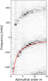 |
Fig. 1. Sectoral power spectrum of the radial vorticity computed from 17.42 years of GONG++ RDA data starting 4 September 2001. Each m is normalized to the mean power between −500 and 100 nHz. For clarity we plot the power spectrum rebinned by a factor of three in frequency. The red line shows the theoretical dispersion relation for sectoral Rossby waves given in the text. While a m = 1 r mode seems to be present, it is likely low-frequency power leaked from m = 0. |
Interestingly, while the m = 2 mode is absent in the spectrum (see also Liang et al. 2019, for a discussion), it appears that there is a peak near the expected frequency of the m = 1 mode in Fig. 1. In order to further investigate this, we performed the same preprocessing on synthetic data (see Appendix A), which show that any yearly variation signal will leak into m = 1 due to the partial coverage of the solar surface (window function). Using the annual variation model of Liang et al. (2019), this leaked signal is removed in our processing. The apparent signal present in m = 1 of Fig. 1 coincides with leakage from low-frequency power in m = 0 and is likely not a true m = 1 r mode.
2.3. Rossby mode parameters
In this section we seek to characterize the r-mode spectrum. The vorticity power spectrum is fit for each of the Rossby modes m assuming the functional form of the Lorentzian,
 (2)
(2)
where S is the mode amplitude, ω0 is the mode frequency, Γ is the full width at half maximum, N is the background noise of the spectrum, and λ = {S, ω0, Γ, N}. The probability density function of the vorticity power spectrum is exponential. As such, the estimates on the parameters λ for each mode are determined by minimizing the negative of the log-likelihood function,
 (3)
(3)
where ωk is the kth frequency bin within the frequency range of interest, consisting of K bins. We use a semi-empirical approach to compute the Hessian and thus the errors on the fit (see Toutain & Appourchaux 1994). The fit for each mode is performed in the frequency range ±300 nHz from the theoretical dispersion relation.
Table 1 lists the fit parameters and their error for the seventeen-year GONG++ RDA r-mode power spectrum. The m = 1 peak is not listed in the table. Its frequency coincides where low-frequency m = 0 power should leak through (421.41 nHz) and has a much smaller amplitude than the other modes. The fit for m = 2 was not performed due to the absence of any signal.
Rossby mode fit parameters for the GONG++ vorticity power spectrum from 2001 to 2019.
2.4. Comparing GONG++ and HMI
In this section we compare the r-mode power spectrum derived from the respective RDA flow map pipelines of HMI and GONG++, for a shared observation period between May 2010 and December 2018. Figure 2 compares the GONG++ and HMI r-mode power spectra for the shared observational period. These results show that while the noise is different, the mode power spectra are in general agreement. The amplitudes of GONG++ and HMI r-mode signals are close, with the GONG++ having a greater background noise. For m > 8 the mode power in the GONG++ data becomes noticably smaller.
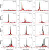 |
Fig. 2. Comparisons of the GONG++ (red) and HMI (black) Rossby wave power spectra for the same observation period of 8 years (2010–2018) using maps of radial vorticity inferred from ring-diagram analysis. The green vertical lines show the measured mode frequencies of Löptien et al. (2018) from granulation tracking data. |
Figure 3 compares the measured frequencies, line widths, vorticity amplitudes, and signal-to-noise ratios (S/Ns) between four different data sets. The data sets include GONG++ and HMI ring diagrams with overlapping observation time, the travel-time results of Liang et al. (2019) derived from time–distance helioseismology, and the LCT results of Löptien et al. (2018). These results show that within error bars the reported mode frequencies and line widths agree for m ≤ 9. For m ≥ 10, the mode frequencies tend not to agree, with the time-distance results of Liang et al. (2019) being shifted towards smaller negative frequencies, while the HMI RDA data analyzed here tend to have greater negative frequencies. In terms of line width, the four spectra tend to be in agreement for all m, though the large reported errors make it difficult to make any strong conclusions on this characteristic of the modes. The HMI and GONG++ RDA mode amplitudes are within error limits for m ≤ 10. However, for higher-order modes HMI data have a greater amplitude by a factor two. Comparing the S/Ns shows that in general the ratio is greater in HMI RDA than GONG++ RDA by a factor of two for m < 8, that S/Ns are similar from m = 8 to m = 11, and that they are greater again for higher-order modes. Our results also show that the S/Ns are significantly higher in ring-diagram data than in travel-time measurements (Liang et al. 2019).
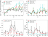 |
Fig. 3. Top left: difference between measured and theoretical resonant frequencies for different data sets: GONG++ RDA (red, 2010–2018), HMI RDA (black, 2010–2018), MDI+HMI time-distance analysis from Liang et al. (2019) (cyan, 1996–2017) and HMI LCT from Löptien et al. (2018) (green, 2010-2016). Top right: measured line widths. Bottom left: measured vorticity amplitudes. Bottom right: measured signal-to-noise ratios. Error bars are one sigma. |
3. Discussion and conclusions
We used 17 years of observations from the ground-based GONG program to characterize solar equatorial Rossby waves. Using ring diagram analysis from the GONG++ pipeline, we clearly identify the solar Rossby waves in the sectoral power spectra of the radial vorticity maps.
Like previous studies we find that the m ≤ 2 r modes are absent from the data. An apparent m = 1 peak appears in the power spectra but we conclude that this peak is leaked through from low-frequency power in m = 0. The synthetics show that a dipole r mode will appear as two peaks separated by 2 × 31.7 nHz due to leakage. No such configuration is seen in the solar spectrum.
With 17 years of near-continuous data, we measured the Rossby mode characteristics. We find that our results, for the period during which GONG++ and HMI data overlap, agree with both Löptien et al. (2018) and Liang et al. (2019) for 4 ≤ m ≤ 9. For m > 9 modes, the GONG++ r-mode frequencies are only in agreement with Löptien et al. (2018). This is due to the chosen method for computing the r-mode spectrum. We find that if we also compute the spectrum through the Fourier transform of uy at the equator, the frequencies agree with Liang et al. (2019). These discrepancies arise for high m because the latitudinal eigenfunctions of the r-modes are not sectoral spherical harmonic functions (Proxauf et al. 2020). Our analysis also suggests that this choice in latitudinal basis function contributes to the small discrepancy for m = 3. The amplitudes from the GONG++ and HMI RDA are within error bars for m ≤ 10. For higher-order modes, the HMI RDA amplitudes are greater than GONG++ by a factor of two. The measured S/Ns of modes in GONG++ RDA power spectra are in the range between 5 and 45. This shows the suitability of the GONG++ data for future studies of global-scale Rossby waves. We note we do not detect any mode in the m = 2 sectoral power spectrum, which is coherent with previous studies.
In this study we focused on only one depth (2 Mm), and measured the mode characteristics for the entire seventeen(or eight)-year time series. We have found good agreement with HMI, despite the lower S/Ns in the GONG++ data. The advantage that GONG++ data has over other data sets is the long and uniform observation window. The next stages for Rossby wave studies should focus on the temporal variation of the waves. With the long time series of GONG shown in this study, and the combined HMI and MDI time series of Liang et al. (2019), the temporal dependence of r-modes could be investigated with two independent data sets.
Acknowledgments
This work was supported by NYUAD Institute Grant G1502. LG acknowledges partial support from the European Research Council Synergy Grant WHOLE SUN 810218. This work utilizes data obtained by the Global Oscillation Network Group (GONG) Program, managed by the National Solar Observatory, which is operated by AURA, Inc. under a cooperative agreement with the National Science Foundation. The HMI data is courtesy of NASA/SDO and the HMI Science Team. CSH thanks Frank Hill and Andrew Marble for their assistance with the GONG data. We also thank Bastian Proxauf and Jishnu Bhattacharya for insightful discussions and Martin Bo Nielsen for performing consistency checks between the analytical fitting of this study and Markov chain Monte Carlo.
References
- Alshehhi, R., Hanson, C. S., Gizon, L., & Hanasoge, S. 2019, A&A, 622, A124 [NASA ADS] [CrossRef] [EDP Sciences] [Google Scholar]
- Beck, J. G., & Giles, P. 2005, ApJ, 621, L153 [NASA ADS] [CrossRef] [Google Scholar]
- Bogart, R. S., Sá, L. A. D., Duvall, T. L., et al. 1995, in Fourth SOHO Workshop: Helioseismology, eds. J. T. Hoeksema, V. Domingo, B. Fleck, B. Battrick, et al., ESA SP-376, 147 [Google Scholar]
- Corbard, T., Toner, C., Hill, F., et al. 2003, in GONG+ 2002. Local and Global Helioseismology: the Present and Future, ed. H. Sawaya-Lacoste, et al., ESA Spec. Pub., 517, 255 [NASA ADS] [Google Scholar]
- Fisher, G. H., & Welsch, B. T. 2008, in Subsurface and Atmospheric Influences on Solar Activity, eds. R. Howe, R. W. Komm, K. S. Balasubramaniam, & G. J. D. Petrie, ASP Conf. Ser., 383, 373 [NASA ADS] [Google Scholar]
- Haber, D. A., Hindman, B. W., Toomre, J., et al. 2000, Sol. Phys., 192, 335 [NASA ADS] [CrossRef] [Google Scholar]
- Hanasoge, S., & Mandal, K. 2019, ApJ, 871, L32 [NASA ADS] [CrossRef] [Google Scholar]
- Hathaway, D. H., & Rightmire, L. 2010, Science, 327, 1350 [NASA ADS] [CrossRef] [Google Scholar]
- Hill, F. 1988, ApJ, 333, 996 [NASA ADS] [CrossRef] [Google Scholar]
- Komm, R., González Hernández, I., Howe, R., & Hill, F. 2015, Sol. Phys., 290, 1081 [NASA ADS] [CrossRef] [Google Scholar]
- Liang, Z.-C., Gizon, L., Birch, A. C., & Duvall, T. L. 2019, A&A, 626, A3 [NASA ADS] [CrossRef] [EDP Sciences] [Google Scholar]
- Löptien, B., Gizon, L., Birch, A. C., et al. 2018, Nat. Astron., 2, 568 [NASA ADS] [CrossRef] [Google Scholar]
- Proxauf, B., Gizon, L., Löptien, B., et al. 2020, A&A, 634, A44 [NASA ADS] [CrossRef] [EDP Sciences] [Google Scholar]
- Saio, H. 1982, ApJ, 256, 717 [NASA ADS] [CrossRef] [Google Scholar]
- Scherrer, P. H., Schou, J., Bush, R. I., et al. 2012, Sol. Phys., 275, 207 [Google Scholar]
- Schou, J., Scherrer, P. H., Bush, R. I., et al. 2012, Sol. Phys., 275, 229 [Google Scholar]
- Toutain, T., & Appourchaux, T. 1994, A&A, 289, 649 [NASA ADS] [Google Scholar]
- Welsch, B. T., Fisher, G. H., Abbett, W. P., & Regnier, S. 2004, ApJ, 610, 1148 [NASA ADS] [CrossRef] [Google Scholar]
Appendix A: Synthetics
In order to quantify the effects of systematics, we generate synthetic Rossby waves and analyze the effects of our data processing (Sect. 2) and the window function due to partial coverage of the Sun. For the functional form of the Rossby waves, we assume they are purely horizontal and obey mass conservation. The flow components  of a sectoral r mode of azimuthal order m are defined by,
 (A.1)
(A.1)
where σm = −2Ωeq/(m + 1) and A = 1 m s−1. Here, Γ/2π is chosen to be 10 nHz. For a single ring-diagram tile the flow components ux and uy can be identified with uϕ and −uθ, respectively. The horizontal flow field within a single tile centered at co-latitude θ and longitude ϕ is then computed by summing the individual r modes:
 (A.2)
(A.2)
 (A.3)
(A.3)
The radial vorticity ζ is then computed through;
![Mathematical equation: $$ \begin{aligned} \zeta (\theta ,\phi ,t) = \frac{1}{R_\odot \sin \theta }\left[ \frac{\partial }{\partial \theta }(u_x\sin \theta ) + \frac{\partial }{\partial \phi }u_{ y}\right] + \frac{A}{R_\odot }\cos ({\omega _\oplus t}) , \end{aligned} $$](/articles/aa/full_html/2020/03/aa37321-19/aa37321-19-eq51.gif) (A.4)
(A.4)
where we added a signal with a yearly period (2π/ω⊕ = 1 year) to emulate the annual systematic error that is present in RDA (e.g., Komm et al. 2015). We limit ourselves to a sum of M = 15 modes.
Using Eq. (A.1), we compute the flows in each 15° tile across the solar surface. We then examine three cases: (1) an ideal case where we have tiles across the entire solar surface at all times; (2) the realistic case when we only have tiles observed by GONG on the visible disk, but no annual variation is removed; and (3) the same as the previous case, except after performing the processing outlined in this paper (e.g., temporal systematic removal).
Figure A.1 shows the sectoral power spectra of the radial vorticity for these three cases. In the ideal case, where the entire sun is observed, we see a clean spectrum without aliasing. In the realistic case (2), there is leakage of modes into their neighboring modes, albeit at frequencies ±421.21 nHz from the central frequency. For the ridge of concern to us, the most significant effect is the leakage into m = 1.
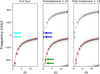 |
Fig. A.1. Sectoral power spectra for the synthetic radial vorticity data for the complete solar surface (full Sun, left panel), including the observational window function (pre-treatment, central panel), and after processing (post-treatment, right panel). Cyan arrows show the peaks at ±(1 year)−1 = ±31.7 nHz. Blue arrows show the leakage of |m| = 1 into m = 0 once the window function is applied. These leakages coincide with the annual variation. After treatment, the annual variation and its leakage disappears, leaving the m = 1 r-modes and associated leakage. The green arrows highlight the effects the window has on m = 1 power. |
All Tables
Rossby mode fit parameters for the GONG++ vorticity power spectrum from 2001 to 2019.
All Figures
|
Fig. 1. Sectoral power spectrum of the radial vorticity computed from 17.42 years of GONG++ RDA data starting 4 September 2001. Each m is normalized to the mean power between −500 and 100 nHz. For clarity we plot the power spectrum rebinned by a factor of three in frequency. The red line shows the theoretical dispersion relation for sectoral Rossby waves given in the text. While a m = 1 r mode seems to be present, it is likely low-frequency power leaked from m = 0. |
| In the text | |
|
Fig. 2. Comparisons of the GONG++ (red) and HMI (black) Rossby wave power spectra for the same observation period of 8 years (2010–2018) using maps of radial vorticity inferred from ring-diagram analysis. The green vertical lines show the measured mode frequencies of Löptien et al. (2018) from granulation tracking data. |
| In the text | |
|
Fig. 3. Top left: difference between measured and theoretical resonant frequencies for different data sets: GONG++ RDA (red, 2010–2018), HMI RDA (black, 2010–2018), MDI+HMI time-distance analysis from Liang et al. (2019) (cyan, 1996–2017) and HMI LCT from Löptien et al. (2018) (green, 2010-2016). Top right: measured line widths. Bottom left: measured vorticity amplitudes. Bottom right: measured signal-to-noise ratios. Error bars are one sigma. |
| In the text | |
|
Fig. A.1. Sectoral power spectra for the synthetic radial vorticity data for the complete solar surface (full Sun, left panel), including the observational window function (pre-treatment, central panel), and after processing (post-treatment, right panel). Cyan arrows show the peaks at ±(1 year)−1 = ±31.7 nHz. Blue arrows show the leakage of |m| = 1 into m = 0 once the window function is applied. These leakages coincide with the annual variation. After treatment, the annual variation and its leakage disappears, leaving the m = 1 r-modes and associated leakage. The green arrows highlight the effects the window has on m = 1 power. |
| In the text | |
Current usage metrics show cumulative count of Article Views (full-text article views including HTML views, PDF and ePub downloads, according to the available data) and Abstracts Views on Vision4Press platform.
Data correspond to usage on the plateform after 2015. The current usage metrics is available 48-96 hours after online publication and is updated daily on week days.
Initial download of the metrics may take a while.