| Issue |
A&A
Volume 635, March 2020
|
|
|---|---|---|
| Article Number | A28 | |
| Number of page(s) | 7 | |
| Section | The Sun and the Heliosphere | |
| DOI | https://doi.org/10.1051/0004-6361/201936938 | |
| Published online | 02 March 2020 | |
Wave heating of the solar atmosphere without shocks
1
Group of Astrophysics, University of Maria Curie-Skłodowska, ul. Radziszewskiego 10, 20-031 Lublin, Poland
e-mail: This email address is being protected from spambots. You need JavaScript enabled to view it.
2
Department of Physics, University of Texas at Arlington, Arlington, TX 76019, USA
3
Leibniz-Institut für Sonnenphysik (KIS), Schöneckstr. 6, 79104 Freiburg, Germany
Received:
17
October
2019
Accepted:
8
January
2020
Abstract
Context. We investigate the wave heating problem of a solar quiet region and present its plausible solution without involving shock formation.
Aims. We aim to use numerical simulations to study wave propagation and dissipation in the partially ionized solar atmosphere, whose model includes both neutrals and ions.
Methods. We used a 2.5D two-fluid model of the solar atmosphere to study the wave generation and propagation. The source of these waves is the solar convection located beneath the photosphere.
Results. The energy carried by the waves is dissipated through ion-neutral collisions, which replace shocks used in some previous studies as the main source of local heating in quiet regions.
Conclusions. We show that the resulting wave dissipation is sufficient to balance radiative and thermal energy losses, and to sustain a quasi-stationary atmosphere whose averaged temperature profile agrees well with the observationally based semi-empirical model of Avrett & Loeser (2008, ApJS, 175, 229).
Key words: Sun: chromosphere / magnetohydrodynamics (MHD) / methods: numerical
© ESO 2020
1. Introduction
The heating problem of the solar atmosphere is very challenging as it requires an explanation of the counter-intuitive 200−500 fold atmospheric temperature rise from about 5600 K at the solar surface over a height of about 2000 km. Two main families of heating mechanisms have been proposed: one uses microflaring while the other is based on energy carried by various waves present in the solar atmosphere. There is observational evidence for the existence of both microflares and waves in the solar atmosphere. The former likely contributes to the heating at higher altitudes, whereas the latter is expected to be responsible for the heating of lower atmospheric layers. The main unsolved heating problem refers to the mechanism by which the wave energy is generated and dissipated. A solution of this longstanding solar physics problem is proposed in this paper.
The most efficient source of waves is the convection zone. Lying below the photosphere, this zone is populated by highly turbulent motions that generate magnetohydrodynamic gravity waves (e.g., Musielak & Ulmschneider 2001). Recent observations reveal a diversity of waves in the solar atmosphere and they also demonstrate that some of these waves carry enough energy to heat this atmosphere (e.g., Jess et al. 2009; Srivastava et al. 2018). Propagation of these waves in the atmosphere is affected by cutoff frequencies. Acoustic-type waves with frequencies higher than their cutoffs are propagating, but waves with lower frequencies are evanescent and their amplitudes decay with height.
The concept of cutoff was originally introduced by Lamb (1909) and later modified to be applicable to the solar atmosphere by others (e.g., Roberts 2004; Musielak et al. 2006). Strong observational evidence for the existence of cutoffs in the atmosphere and their variations with the atmospheric height was presented by Wiśniewska et al. (2016) and Kayshap et al. (2018). Several theoretical attempts have been made to fit the available observational data (e.g., Murawski et al. 2016; Wójcik et al. 2018) without achieving satisfactory agreement. However, in the most recent study by Wójcik et al. (2019a), good agreement between the numerical simulations and observations was finally achieved, and the authors pointed out the importance of partially ionized effects that were accounted for by their numerical code. Similar code is used in this paper but with the exception that all nonideal and nonadiabatic terms are switched on. However, the main goal of this paper is different from that of Wójcik et al., as here we concentrate on wave generation and dissipation, and the solar atmosphere wave heating problem.
Waves in the solar atmosphere may form shocks that heat the plasma locally (e.g., Ulmschneider et al. 1978; Carlsson & Stein 1995). Fawzy et al. (2002) constructed theoretical models of the chromosphere that are based on the waves generated in the convection zone and using the dissipation of wave energy by shock formation (Hillier et al. 2016). The constructed models were purely theoretical, one-dimensional (1D) and they included both nonmagnetic and magnetic regions as well as full treatment of nonlocal thermodynamic equilibrium (NLTE) ionization and radiation. The only free parameter in these models was a filling factor, which was used to explain different levels of activity observed in solar-like stars. The models were used to compute profiles of Ca II and Mg II lines, which were compared to observational data. The comparison shows good agreement between the theoretically predicted line profiles and observations, and also demonstrates that the theoretically predicted temperature variations in the solar atmosphere are in an agreement with the semi-empirical VAL model (Vernazza et al. 1981). The main difference between the approach of Hillier et al., which was based on fully ionized plasma, and the one presented in this paper is that our numerical model is 2D and properly accounts for partially ionized plasma in the solar atmosphere.
In the chromosphere models described above, and in most of the previous theoretical studies, i.e., studies of Hillier et al. (2016), the effects of partially ionized plasma in the gravitationally stratified solar atmosphere were often neglected or considered under some assumptions. For instance, Wójcik et al. (2018) and Kuźma et al. (2019) devised 1D models of the dynamics of ions and neutrals and then the models were extended to 2D geometry (e.g., Srivastava et al. 2018; Wójcik et al. 2019a,b). Moreover, Maneva et al. (2017) developed a 2D model of nonadiabatic and nonideal atmosphere to show that ion magnetoacoustic-gravity and neutral acoustic-gravity waves (e.g., Vigeesh et al. 2017) lead to local heating of a magnetic flux tube. In addition, Martínez-Sykora et al. (2017) and Khomenko et al. (2018) included neutrals in their respectively 2D and 3D models of self-generated solar granulation. The contribution of neutrals was taken into account by amending a few extra terms in the induction equation. These models were recently generalized to dynamic ions and neutrals in the chromosphere by Popescu Braileanu et al. (2019) who reported the development of a new two-fluid code and its numerical verification. We present here an approach in which ions and neutrals are included self-consistently in our numerical model, and their dynamical effects on wave propagation and dissipation are fully accounted for. Our approach provides new insight into the wave heating problem.
Our paper is organized as follows: our two-fluid (ions + electrons and neutrals) model is described in Sect. 2; wave heating resulting from our numerical simulations is presented and discussed in Sect. 3; our conclusions are given in Sect. 4
2. Two-fluid model of a partially ionized solar atmosphere
We consider a gravitationally stratified and partially ionized solar atmosphere whose evolution is described by the set of two-fluid equations (e.g., Zaqarashvili et al. 2011; Leake et al. 2012; Martínez-Gómez et al. 2018; Soler et al. 2013; Oliver et al. 2016; Ballester et al. 2018, and references therein). We take into account hydrogen as a main dynamic plasma ingredient; the influence of heavier plasma species is considered with use of the OPAL solar abundance model (e.g., Vögler et al. 2004). Additionally, for simplicity we assume that ions and electrons consist of a single ion-electron fluid, while neutrals are described by a second fluid. Interaction between both fluids occurs through the ion–neutral collisions. In this model we neglect effects of recombination, ionization, and charge exchange, as well as effects of electrons exerted on ions, mimicked by extra terms in the generalized Ohm’s law (e.g., Khomenko 2017). As a result of complexity of the present model, these effects are left for future studies.
2.1. Two-fluid equations for ions and neutrals
We write the equations that describe dynamics of neutral and ion + electron fluids as
 (1)
(1)
 (2)
(2)
 (3)
(3)
 (4)
(4)
 (5)
(5)
![Mathematical equation: $$ \begin{aligned}&\frac{\partial E_{\rm n}}{\partial t}+\nabla \cdot [(E_{\rm n}+p_{\rm n}){\boldsymbol{V}}_{\rm n}]\nonumber \\&\qquad \qquad =\alpha _c{\boldsymbol{V}}_{\rm n} \cdot ({\boldsymbol{V}}_{\rm i}-{\boldsymbol{V}}_{\rm n}) +Q_{\rm n} ^\mathrm{in} + q_{\rm n} + \varrho _{\rm n} {\boldsymbol{g}} \cdot {\boldsymbol{V}}_{\rm n}, \end{aligned} $$](/articles/aa/full_html/2020/03/aa36938-19/aa36938-19-eq6.gif) (6)
(6)
![Mathematical equation: $$ \begin{aligned}&\frac{\partial E_{\rm i}}{\partial t}+\nabla \cdot \left[\left(E_{\rm i}+p_{\rm ie} + \frac{{\boldsymbol{B}}^2}{2\mu } \right){\boldsymbol{V}}_{\rm i}-\frac{{\boldsymbol{B}}}{\mu }({\boldsymbol{V}}\cdot {\boldsymbol{B}})\right]\nonumber \\&\qquad \qquad =\alpha _c {\boldsymbol{V}}_{\rm i} \cdot ({\boldsymbol{V}}_{\rm n}-{\boldsymbol{V}}_{\rm i}) + Q_{\rm i}^\mathrm{in} + Q^i_{R} + q_{\rm i} + \varrho _{\rm i} {\boldsymbol{g}} \cdot {\boldsymbol{V}}_{\rm i}, \end{aligned} $$](/articles/aa/full_html/2020/03/aa36938-19/aa36938-19-eq7.gif) (7)
(7)
where the heat production terms are
 (8)
(8)
 (9)
(9)
with ΔV = Vi − Vn, ΔT = Ti − Tn, and a = 3kB/(mH(μi+μn)). Here I is the identity matrix, and subscripts i, n, and e correspond respectively to ions, neutrals, and electrons. The symbols 𝜚i, n denote mass densities, Vi, n velocities, pie, n ion + electron and neutral gas pressures, B magnetic field, and Ti, n are temperatures specified by ideal gas laws,
 (10)
(10)
where the gravity vector is g = [0, −g, 0] with its magnitude g = 274.78 m s−2, αc is the coefficient of collisions between ion and neutral particles, qi, n describe thermal conduction (Spitzer 1962),  represents radiative losses, μie = 0.58 and μn = 1.21 are the mean masses of electrons + ionized plasma species and neutrals, respectively, and they are taken from the OPAL solar abundance model (e.g., Vögler et al. 2004), mH is the hydrogen mass, kB is the Boltzmann constant, γ = 1.4 is the specific heats ratio, and μ is the magnetic permeability of the medium. All other symbols have their standard meaning.
The radiative losses term,  , consists of two separate parts: thick cooling which operates in the low atmospheric layers and thin cooling, which works in the upper atmospheric regions. In every time-step we calculate the optical depth, starting from infinity and ending at the bottom boundary. For optical depths higher than 0.1 we use the thick cooling approximation of Abbett & Fisher (2012). For optical depths lower than 0.1 we use the thin cooling curve (Cox & Tucker 1969), which is interpolated by a tenth-order polynomial. In order to mimic energy transport into the simulation box from lower lying convective regions, we supplemented the radiative term by the heating term which overwhelms cooling by 5% at optical depths τ > 10.
Following Zaqarashvili et al. (2011), we assume coefficient of collisions between ions and neutrals αin = αni = αc, and to estimate its value we use the following formula provided by Braginskii (1965):
 (11)
(11)
Here the collisional cross-section σin is taken from the quantum-mechanical model of Vranjes & Krstic (2013) who showed that the classical hard-sphere model may lead to underestimation of the cross-section values. For typical chromospheric plasma temperature in the range of 6 × 10³ − 104 K this cross-section is equal to 1.89 × 10⁻¹⁸ m2, that is about three orders of magnitude larger than in the hard-sphere model. We experienced for acoustic waves that the released heating due to ion-neutral collisions is higher for the classical cross-section than for its quantum analog (Kuźma et al. 2019). We note that the ion–neutral collision frequency differs from the neutral–ion collision frequency (Ballester et al. 2018), and they are given as νin = αc/𝜚i and νni = αc/𝜚n, respectively.
2.2. Initial hydrostatic equilibrium of the solar atmosphere
Here, we consider the initial conditions of the solar atmosphere. We assume that the atmosphere is initially in hydrostatic (Vi, n = 0) equilibrium. The equilibrium mass density profiles of ions and neutrals (Fig. 1) are specified uniquely by the temperature profile, which is taken to be the same for ions and neutrals (e.g., Oliver et al. 2016) from the quiet solar atmosphere model of Avrett & Loeser (2008). We note that the ion mass density is much lower than the neutral mass density in the photosphere and the low chromosphere; they become comparable about 900 km below the transition region which is located at y ≈ 2.1 Mm. Higher up, the neutrals are less abundant than ions; in the corona the mass density of neutrals experiences a sudden fall-off with height. As a result of ion and neutral distributions, the ionization degree depends on height in the solar atmosphere; in the photosphere, where the temperature is only about 5800 K, the plasma is very weakly ionized with only about one ion for every thousand neutrals, while in the solar corona the plasma there is essentially fully ionized.
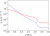 |
Fig. 1. Initial vertical profiles of ion, 𝜚i, (solid line) and neutral, 𝜚n, (dashed line) mass densities. |
Interaction between ion + electron and neutral fluids occurs through the ion–neutral collisions that are determined by the ion–neutral friction coefficient (Eq. (11)). Vertical profile of αc is illustrated in Fig. 2 (left). Below the photosphere, αc retains its high value of 20 km s−1, and therefore both fluids are strongly coupled there, acting as a single fluid as a result. At the bottom of the photosphere, that is at y = 0, the value of αc begins to decrease with altitude. Higher up, both fluids decouple, enabling ion-neutral drift, ΔV = Vi − Vn, to take place in the chromospheric and transition region layers. This drift is essential for collisional heating (Eqs. (8) and (9)). The sound speed cs can be given as
 (12)
(12)
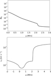 |
Fig. 2. Vertical profiles of ion-neutral friction coefficient, αc, (left panel) and sound speed, cs, (right panel) in units of g cm−3 s−1 and km s−1. |
In the photosphere, cs is close to 6 km s−1 (Fig. 2, right). Immediately below the transition region, cs(y = 2 Mm) ≈ 11 km s−1. Higher up, cs grows, following the trend of  ; this growth is abrupt immediately above the transition region, and at larger altitudes cs rises slowly to a value of about 150 km s−1 at y ≈ 30 Mm (not shown).
We adopt here the uniform magnetic field with its vertical and transverse components given as B = [0, B0, B0] with  Gs. A nonzero transversal magnetic field permits transversal Alfvén waves to be present in the system. These waves are linearly coupled to magnetoacoustic waves and are essential in the model; as in the nonlinear regime they are capable of driving vertical flow (e.g., Hollweg 1986; Murawski 1992; Shestov et al. 2017). The mode conversion between slow-acoustic and Alfvén modes in regions of β ≈ 1 can take place in this system. A nonlinear coupling between slow and Alfvén waves near these regions has been studied by Zaqarashvili & Roberts (2006). A detailed discussion on two-fluid Alfvén waves can be found in Kuźma et al. (in prep.). The vertical profile of the corresponding Alfvén speed,
  , is illustrated in Fig. 3. In the upper photosphere and lower chromosphere, cA attains values lower than 10 km s−1 up to y ≈ 1 Mm. Higher-up, as a result of low ion mass density 𝜚i, cA rises until the transition region, where it experiences a sudden growth to values close to 800 km s−1.
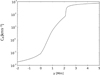 |
Fig. 3. Profile of the initial Alfvén speed, cA, versus height y. |
3. Numerical simulations of two-fluid wave heating
We use JOANNA code (Wójcik et al. 2018) to solve the two-fluid equations numerically. We set in our numerical experiments the Courant-Friedrichs-Lewy (Courant et al. 1928) number equal to 0.3 and choose a second-order accuracy in space and a second-order accurate Runge-Kutta method (Durran 2010) for integration in time, supplemented by adopting the Harten-Lax-van Leer discontinuities (HLLD) approximate Riemann solver (Miyoshi & Kusano 2005) and the divergence of magnetic field cleaning method of Dedner et al. (2002).
The simulation box is specified along horizontal (x-) and vertical (y-) directions as ( − 5.12 < x < 5.12) Mm × ( − 5.12 < y < 30) Mm. This allows us to simulate a convectively unstable region just below the photosphere which occupies the layer 0 ≤ y ≤ 0.5 Mm. Below the height y = 5.12 Mm, we set a uniform grid with cell size 20 km × 20 km, while higher up at the base of the corona, which is located at y = 2.1 Mm, we stretch the grid along the y-direction dividing it into cells whose size grows with height. Two different types of boundary conditions are implemented at four edges of the simulation box. All plasma quantities at the top and bottom boundaries are set to their hydrostatic values. At the right and left boundary we use periodic boundary conditions. With the use of the stretched grid above y = 5.12 Mm we damp any incoming signal in layers close to the upper boundary. We find that such a stretched grid, supplemented by fixing all plasma quantities to their hydrostatic conditions at the top boundary, significantly reduces spurious reflections of the incoming signal. Additionally, we implemented a plasma inflow at the bottom boundary with its vertical velocity equal to 0.3 km s−1. This allows us to compensate the outflowing plasma mass losses. The value of inflow velocity is calculated by assuming that the incoming flux compensates the radiative losses (Chatterjee 2020).
In our numerical simulations we consider plasma that is initially (at t = 0 s) set to its hydrostatic state with the vertical and transverse components of magnetic field equal to  Gs. Later on, horizontal motions of plasma due to spontaneously generated granulation reshuffle magnetic field lines in the photosphere in the form of small flux tubes (Fig. 4, solid lines). These horizontal plasma motions reveal mean velocity close to 2.5 km s−1 at y = 0 Mm (not shown) with a maximum value of up to 5 km s−1, and thus they remain subsonic. This figure also reveals the presence of a well-defined cool and dynamic chromosphere above the photosphere. This chromosphere layer is filled with both hot and cold jets visible at x ≈ 2.5 Mm.
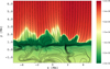 |
Fig. 4. Spatial profile of logarithm of ion temperature, Ti, expressed in units of Kelvins (colormap) overlayed by magnetic field lines at t = 5000 s. |
Hot plasma associated with granulation (Fig. 4, colormap) drifts towards the chromosphere and forms plasma upflows (Fig. 5, top). At the bottom of the chromosphere this plasma radiates its energy and gets cooled. Between sibling granules the downdrafts with cold plasma flowing down settle in the convection zone (Fig. 5, top). Both these upflows and downdrafts are accompanied by two-fluid waves (Fig. 5, bottom), which in our model atmosphere are neutral acoustic-gravity, ion magnetoacoustic-gravity (Vigeesh et al. 2017), and Alfvén waves.
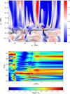 |
Fig. 5. Spatial profile of the vertical component of ion velocity, Vi, expressed in units of 1 km s−1 (top) and its spatially averaged Fourier power periods vs. height (bottom) at t = 5000 s. |
The periods of the excited waves, which we obtained from the Fourier spectra for ion vertical velocity, are plotted in Fig. 5 (bottom). We note that at the height within the range of 0 Mm < y < 0.5 Mm, the dominant wave period P is about 340 s. However, higher up, for y > 0.5 Mm, the signal associated with large values of P decays fast with y, and the main wave period is associated with P ≈ 180 s. It was demonstrated that acoustic waves of P ≈ 300 s are evanescent in the photosphere (e.g., Wójcik et al. 2018) but they are filtered out in higher layers. Thus, the package of waves consists of the main wave-period of about 180 s (Fig. 5, bottom). The described filtering process dominates in the chromosphere and it lowers periods and allows the waves to reach the transition region located at y = 2.1 Mm, where the waves become partially reflected back to the chromosphere. As a result of ion–neutral collisions, the energy of these excited waves is dissipated. This dissipation is most effective for largest dispatches between ion and neutral velocities, and these waves may convert their energy into heat mostly in the chromosphere (Fig. 6), compensating radiative and thermal losses.
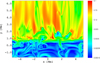 |
Fig. 6. Spatial profile of the absolute difference between ion and neutral velocities (|Vi − Vn|) expressed in units of 1 km s−1 at t = 5000 s. |
A strong damping of low-frequency (with period > 80 s) Alfvén waves does not follow the conclusions drawn from the analytical studies of Zaqarashvili et al. (2013) who showed that waves with short wave-periods are rapidly damped by ion–neutral collisions. However, our two-fluid model describes highly dynamic solar atmosphere (that nevertheless remains in quasi-equilibrium) and differs significantly from those developed so far. A signal present in Viz is partially converted through ion-neutral collisions into a signal in Vnz. It follows from the dispersion relation that Vnz is associated with a purely imaginary frequency which corresponds to a strongly damped wave (Zaqarashvili et al. 2013). This effect along with the energy transfer from Viy into Vnz causes Alfvén waves, which correspond to Viz, to be strongly damped. We found that longer wave periods are not the main cause of the heating of the solar atmosphere, which agrees with the numerical results of Kuźma et al. (2019) who found that for acoustic waves, with wave periods longer than 80 s, the plasma heating decreases.
Figure 7 shows the vertical profile of horizontally averaged ionization, 𝜚i/𝜚n, at three moments of time, namely t = 0 s (solid line), that is, initial ionization, t = 2000 s (dashed line), and t = 4000 s (dotted line), which corresponds to fully developed and ongoing granulation. From this plot we can see, that 𝜚i/𝜚n drops by about one order of magnitude in the upper chromosphere. The ionization levels in the photosphere, lower chromosphere, and corona remain close to their initial values.
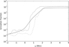 |
Fig. 7. Horizontally averaged vertical profile of ionization fraction, 𝜚i/𝜚n, at t = 0 s (solid line), t = 2000 s (dashed line) and t = 4000 s (dash-dotted line). |
The numerically obtained quasi-stationary solar atmosphere is the result of the subtle balance between radiative cooling, thermal conduction, and collisional energy dissipation mechanism. This equilibrium is illustrated in Fig. 8 in the form of horizontally averaged collisional heating and negative cooling rates versus height. We note that by definition, the heating rate attains positive values, while cooling negative values. Deep below the photosphere, heating from the deeper layers overcomes cooling, and leads to hot plasma upflows in the convectively unstable layer. At the photosphere, that is for 0 < y < 0.5 Mm, the optical opacity abruptly falls off and hot plasma rapidly radiates its energy. Thereafter, the heating term overwhelms the cooling term in this layer. Higher up, that is, in the chromosphere and low corona, these two terms reach a similar value, with the cooling term being slightly dominant in the corona. It is demonstrated that the wave energy dissipation, which is supplemented by viscous and ohmic heatings, is sufficient to balance radiative and thermal energy losses above the photosphere and to sustain a quasi-stationary solar atmosphere.
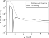 |
Fig. 8. Horizontally averaged vertical profiles of collisional heating (dotted line) and minus cooling term (solid line) vs. height y, drawn at t = 5000 s. |
Figure 9 shows the temporal evolution of horizontally averaged Ti. We see that, as a result of cooling–heating balance in the chromosphere, the system arrives at a quasi-equilibrium state of the solar atmosphere. The chromosphere in our simulations is a highly dynamic medium filled with jets and spicules that transport mass to balance losses due to plasma outflows (Wójcik et al. 2019b). The well-defined transition region oscillates close to its initial position at y = 2.1 Mm.
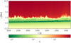 |
Fig. 9. Time distance plot of the horizontally averaged Ti. |
Figure 10 reveals that the radiative cooling and thermal energy losses are in equilibrium with collisional heating, sustaining a quasi-stationary atmosphere with the transition region located around y = 2.1 Mm. As a result of this balance, the numerically obtained vertical profile of ion temperature is close to the semi-empirical data of Avrett & Loeser (2008). A better fit would require tuning the inflow or the extra heating which we impose below the photosphere. However, such parametric studies are very costly as they require a number of jobs to be run. It must be pointed out that this agreement was obtained without invoking shocks, which were previously considered as the main source of local heating in the solar chromosphere (e.g., Ulmschneider et al. 1978; Carlsson & Stein 1995; Fawzy et al. 2002). Such shocks are occasionally generated in the upper chromosphere. However, our results show that the efficient wave heating by ion-neutral collisions prevents shock formation in the lower and middle chromosphere. Thus, a new insight into the wave heating problem is our demonstration that the waves dissipate their energy without forming shocks; another important aspect of this result is that short-period waves, which were the main source of heating of the lower chromosphere in the latter mentioned study, can now reach much higher layers of the chromosphere, including the transition region and corona. Our results allow us to obtain an average temperature distribution that is very similar to that in the semi-empirical model of Avrett & Loeser (2008), which is good confirmation of the validity of our approach and the code used to perform the simulations. Moreover, we also demonstrate that the ion temperature varies locally in the chromosphere, and the predicted range is consistent with the results of the numerical simulations reported by Carlsson & Stein (1995). The latter study shows that temperature variation grows with height, attaining the greatest values in the low corona. Figure 10 presents a similar trend, although the temperature variations are smaller than those of Carlsson & Stein (1995), which may result from the presence of ions and neutrals in the model we developed.
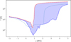 |
Fig. 10. Numerically obtained minimum Ti(y) (blue dashed line) and maximum Ti(y) (red dashed line) at x = 0, and semi-empirical data of T(y) of Avrett & Loeser (2008; dotted line). |
Recent observations of Grant et al. (2018) showed that Alfvén waves are steepening into shocks at lower heights of the solar atmosphere. With observed local temperature enhancements of 5% it is the first observational evidence of Alfvén waves heating chromospheric plasma in a sunspot umbra through the formation of shock fronts. In our simulations, thermal energy is released during collisions between ions and neutrals which may lead to ion–neutral velocity drift, and this is a pure two-fluid effect. In the case of a shock, kinetic energy at the front of this shock is converted to thermal energy as a result of the friction between ion + electron fluid and neutral species. This phenomenon takes place not only at a shock but also at all other waves in general. However, it is more efficient for steeper wave profiles and its impact on overlaying plasma temperature depends on ion–neutral drift. In conclusion, it is therefore largest in the case of shocks.
Finally, it must also be emphasized that similar code was used by Wójcik et al. (2019a,b) to propose that the solar wind origin is associated with granulation, and to theoretically predict the variations of acoustic cutoff frequency in the solar atmosphere, which are in good agreement with the observational results obtained by Wiśniewska et al. (2016) and Kayshap et al. (2018). This is another independent verification of the validity of our approach and the code, and it shows that the effects of partial ionization become very important in lower and middle chromospheric layers.
4. Conclusions
We performed numerical simulations of two-fluid waves in a partially ionized solar atmosphere with radiation and thermal conduction taken self-consistently into account. The considered neutral acoustic-gravity, Alfvén, and ion magnetoacoustic gravity waves were generated by spontaneously evolving and self-organizing convection with granulation cells. We found that the granulation excites a wide spectrum of wave periods (Fig. 5, bottom) and that only sufficiently short-period acoustic and long-period gravity waves propagate through the atmosphere and reach the corona (Vigeesh et al. 2017).
Part of the energy carried by these waves is dissipated in the photosphere and chromosphere because of ion–neutral collisions. As a result, these two-fluid waves generated by the granulation effectively heat the plasma, compensating radiative and thermal energy losses there. The atmosphere also gets extra heat from viscosity and magnetic diffusivity, which are most effective at the places of sheared flow and oppositely orientated magnetic field lines. This heating takes place at the downdrafts below the photosphere, contributing to plasma temperatures there and leading to a quasi-stationary solar atmosphere with its temperature distribution being close to the semi-empirical model of Avrett & Loeser (2008).
This is the first time that agreement with the observationally based semi-empirical model has been obtained without involving heating by shocks. We conclude that our results unravel the main mechanism of the wave heating quiet regions of the chromosphere, and that the basic physical process of this mechanism is collisions between neutrals and ions. Our results have important implications for the construction of theoretical solar atmospheric models in the near future as they show that the effects of partially ionized plasma must be included in these models and that they may prevent shock formation, which was a dominant physical process for waves in a fully ionized solar atmosphere.
Acknowledgments
The JOANNA code was developed by Darek Wójcik at UMCS. This work was done within the framework of the projects from the Polish Science Center (NCN) Grant Nos. 2017/25/B/ST9/00506 and 2017/27/N/ST9/01798.
References
- Abbett, W. P., & Fisher, G. H. 2012, Sol. Phys., 277, 3 [Google Scholar]
- Avrett, E., & Loeser, R. 2008, ApJS, 175, 229 [NASA ADS] [CrossRef] [Google Scholar]
- Ballester, J. L., Alexeev, I., Collados, M., et al. 2018, Space Sci. Rev., 214, 58 [NASA ADS] [CrossRef] [Google Scholar]
- Braginskii, S. 1965, Rev. Plasma Phys., 1, 205 [NASA ADS] [Google Scholar]
- Carlsson, M., & Stein, R. F. 1995, ApJ, 440, L29 [NASA ADS] [CrossRef] [Google Scholar]
- Chatterjee, P. 2020, J. Geophys. Astrophys. Fluid Dyn., 114, 213 [NASA ADS] [CrossRef] [Google Scholar]
- Courant, R., Friedrichs, K., & Lewy, H. 1928, Math. Ann., 100, 32 [NASA ADS] [CrossRef] [MathSciNet] [Google Scholar]
- Cox, D. P., & Tucker, W. H. 1969, ApJ, 157, 1157 [NASA ADS] [CrossRef] [Google Scholar]
- Dedner, A., Kemm, F., Kröner, D., et al. 2002, J. Comput. Phys., 175, 645 [Google Scholar]
- Durran, D. R. 2010, Numerical Methods for Fluid Dynamics (New York: Springer) [CrossRef] [Google Scholar]
- Fawzy, D., Stȩpień, K., Ulmschneider, P., et al. 2002, A&A, 386, 994 [NASA ADS] [CrossRef] [EDP Sciences] [Google Scholar]
- Grant, S. D. T., Jess, D. B., Zaqarashvili, T. V., et al. 2018, Nat. Phys., 14, 480 [CrossRef] [Google Scholar]
- Hillier, A., Takasao, S., & Nakamura, N. 2016, A&A, 591, A112 [NASA ADS] [CrossRef] [EDP Sciences] [Google Scholar]
- Hollweg, J. V. 1986, ApJ, 306, 730 [NASA ADS] [CrossRef] [Google Scholar]
- Jess, D. B., Mathioudakis, M., Erdélyi, R., et al. 2009, Science, 323, 1582 [NASA ADS] [CrossRef] [PubMed] [Google Scholar]
- Kayshap, P., Murawski, K., Srivastava, A. K., et al. 2018, MNRAS, 479, 5512 [NASA ADS] [CrossRef] [Google Scholar]
- Khomenko, E. 2017, Plasma Phys. Controll. Fusion, 59, 014038 [NASA ADS] [CrossRef] [Google Scholar]
- Khomenko, E., Vitas, N., Collados, M., et al. 2018, A&A, 618, A87 [NASA ADS] [CrossRef] [EDP Sciences] [Google Scholar]
- Kuźma, B., Wójcik, D., & Murawski, K. 2019, ApJ, 878, 81 [NASA ADS] [CrossRef] [Google Scholar]
- Lamb, H. 1909, Proc. London Math. Soc., 7, 122 [Google Scholar]
- Leake, J. E., Lukin, V. S., Linton, M. G., & Meier, E. T. 2012, ApJ, 760, 109 [NASA ADS] [CrossRef] [Google Scholar]
- Maneva, Y. G., Alvarez Laguna, A., Lani, A., et al. 2017, ApJ, 836, 197 [NASA ADS] [CrossRef] [Google Scholar]
- Martínez-Sykora, J., Pontieu, B. D., Hansteen, V. H., et al. 2017, Science, 356, 1269 [NASA ADS] [CrossRef] [Google Scholar]
- Martínez-Gómez, D., Soler, R., & Terradas, J. 2018, ApJ, 856, 16 [NASA ADS] [CrossRef] [Google Scholar]
- Miyoshi, T., & Kusano, K. 2005, J. Comput. Phys., 208, 315 [NASA ADS] [CrossRef] [Google Scholar]
- Murawski, K. 1992, Sol. Phys., 139, 279 [NASA ADS] [CrossRef] [Google Scholar]
- Murawski, K., Musielak, Z. E., Konkol, P., et al. 2016, ApJ, 827, 37 [NASA ADS] [CrossRef] [Google Scholar]
- Musielak, Z. E., & Ulmschneider, P. 2001, A&A, 370, 541 [NASA ADS] [CrossRef] [EDP Sciences] [Google Scholar]
- Musielak, Z. E., Musielak, D. E., & Mobashi, H. 2006, Phys. Rev. E, 73, 036612 [NASA ADS] [CrossRef] [Google Scholar]
- Oliver, R., Soler, R., Terradas, J., & Zaqarashvili, T. V. 2016, ApJ, 818, 128 [NASA ADS] [CrossRef] [Google Scholar]
- Popescu Braileanu, B., Lukin, V. S., Khomenko, E., et al. 2019, A&A, 627, A25 [NASA ADS] [CrossRef] [EDP Sciences] [Google Scholar]
- Roberts, B. 2004, in Proceedings of “SOHO 13 Waves, Oscillations and Small-scale Transients Events in the Solar Atmosphere: Joint View from SOHO and TRACE”, ed. H. Lacoste, 1 [Google Scholar]
- Shestov, S. V., Nakariakov, V. M., Ulyanov, A. S., Reva, A. A., & Kuzin, S. V. 2017, ApJ, 840, 64 [NASA ADS] [CrossRef] [Google Scholar]
- Soler, R., Carbonell, M., & Ballester, J. L. 2013, ApJS, 209, 16 [NASA ADS] [CrossRef] [Google Scholar]
- Spitzer, L. 1962, Physics of Fully Ionized Gases (New York: Dover) [Google Scholar]
- Srivastava, A. K., Murawski, K., Kuźma, B., et al. 2018, Nat. Astron., 2, 951 [Google Scholar]
- Ulmschneider, R., Schmitz, F., Kalkofen, W., et al. 1978, A&A, 70, 487 [NASA ADS] [Google Scholar]
- Vernazza, J. E., Avrett, E. H., & Loeser, R. 1981, ApJS, 45, 635 [NASA ADS] [CrossRef] [Google Scholar]
- Vigeesh, G., Jackiewicz, J., & Steiner, O. 2017, ApJ, 835, 148 [NASA ADS] [CrossRef] [Google Scholar]
- Vögler, A., Bruls, J. H. M. J., & Schüssler, M. 2004, A&A, 421, 741 [NASA ADS] [CrossRef] [EDP Sciences] [Google Scholar]
- Vranjes, J., & Krstic, P. S. 2013, A&A, 554, A22 [NASA ADS] [CrossRef] [EDP Sciences] [Google Scholar]
- Wiśniewska, A., Musielak, Z. E., Staiger, J., et al. 2016, ApJ, 819, L23 [Google Scholar]
- Wójcik, D., Murawski, K., & Musielak, Z. E. 2018, MNRAS, 481, 262 [NASA ADS] [CrossRef] [Google Scholar]
- Wójcik, D., Murawski, K., & Musielak, Z. E. 2019a, ApJ, 882, 1 [CrossRef] [Google Scholar]
- Wójcik, D., Kuźma, B., Murawski, K., & Srivastava, A. K. 2019b, ApJ, 884, 2 [NASA ADS] [CrossRef] [Google Scholar]
- Zaqarashvili, T. V., & Roberts, B. 2006, A&A, 452, 1053 [NASA ADS] [CrossRef] [EDP Sciences] [Google Scholar]
- Zaqarashvili, T. V., Khodachenko, M. L., & Rucker, H. O. 2011, A&A, 534, A93 [NASA ADS] [CrossRef] [EDP Sciences] [Google Scholar]
- Zaqarashvili, T. V., Khodachenko, M. L., & Soler, R. 2013, A&A, 549, A113 [NASA ADS] [CrossRef] [EDP Sciences] [Google Scholar]
All Figures
|
Fig. 1. Initial vertical profiles of ion, 𝜚i, (solid line) and neutral, 𝜚n, (dashed line) mass densities. |
| In the text | |
|
Fig. 2. Vertical profiles of ion-neutral friction coefficient, αc, (left panel) and sound speed, cs, (right panel) in units of g cm−3 s−1 and km s−1. |
| In the text | |
|
Fig. 3. Profile of the initial Alfvén speed, cA, versus height y. |
| In the text | |
|
Fig. 4. Spatial profile of logarithm of ion temperature, Ti, expressed in units of Kelvins (colormap) overlayed by magnetic field lines at t = 5000 s. |
| In the text | |
|
Fig. 5. Spatial profile of the vertical component of ion velocity, Vi, expressed in units of 1 km s−1 (top) and its spatially averaged Fourier power periods vs. height (bottom) at t = 5000 s. |
| In the text | |
|
Fig. 6. Spatial profile of the absolute difference between ion and neutral velocities (|Vi − Vn|) expressed in units of 1 km s−1 at t = 5000 s. |
| In the text | |
|
Fig. 7. Horizontally averaged vertical profile of ionization fraction, 𝜚i/𝜚n, at t = 0 s (solid line), t = 2000 s (dashed line) and t = 4000 s (dash-dotted line). |
| In the text | |
|
Fig. 8. Horizontally averaged vertical profiles of collisional heating (dotted line) and minus cooling term (solid line) vs. height y, drawn at t = 5000 s. |
| In the text | |
|
Fig. 9. Time distance plot of the horizontally averaged Ti. |
| In the text | |
|
Fig. 10. Numerically obtained minimum Ti(y) (blue dashed line) and maximum Ti(y) (red dashed line) at x = 0, and semi-empirical data of T(y) of Avrett & Loeser (2008; dotted line). |
| In the text | |
Current usage metrics show cumulative count of Article Views (full-text article views including HTML views, PDF and ePub downloads, according to the available data) and Abstracts Views on Vision4Press platform.
Data correspond to usage on the plateform after 2015. The current usage metrics is available 48-96 hours after online publication and is updated daily on week days.
Initial download of the metrics may take a while.