| Issue |
A&A
Volume 635, March 2020
|
|
|---|---|---|
| Article Number | A67 | |
| Number of page(s) | 18 | |
| Section | Interstellar and circumstellar matter | |
| DOI | https://doi.org/10.1051/0004-6361/201936714 | |
| Published online | 10 March 2020 | |
What determines the formation and characteristics of protoplanetary discs?
1
AIM, CEA, CNRS, Université Paris-Saclay, Université Paris Diderot,
Sorbonne Paris Cité,
91191
Gif-sur-Yvette,
France
e-mail: This email address is being protected from spambots. You need JavaScript enabled to view it.
2
Institut de Physique du Globe de Paris, Sorbonne Paris Cité, Université Paris Diderot, UMR 7154 CNRS,
75005
Paris,
France
3
Univ Lyon, Ens de Lyon, Univ Lyon1, CNRS, Centre de Recherche Astrophysique de Lyon UMR5574,
69007
Lyon, France
4
Department of Earth Sciences, National Taiwan Normal University,
88, Sec. 4, Ting-Chou Road,
Taipei
11677,
Taiwan
Received:
17
September
2019
Accepted:
25
December
2019
Abstract
Context. Planets form in protoplanetary discs. Their masses, distribution, and orbits sensitively depend on the structure of the protoplanetary discs. However, what sets the initial structure of the discs in terms of mass, radius and accretion rate is still unknown.
Aims. It is therefore of great importance to understand exactly how protoplanetary discs form and what determines their physical properties. We aim to quantify the role of the initial dense core magnetisation, rotation, turbulence, and misalignment between rotation and magnetic field axis as well as the role of the accretion scheme onto the central object.
Methods. We performed non-ideal magnetohydrodynamics numerical simulations using the adaptive mesh refinement code Ramses of a collapsing, one solar mass molecular core to study the disc formation and early, up to 100 kyr, evolution. We paid particular attention to the impact of numerical resolution and accretion scheme.
Results. We found that the mass of the central object is almost independent of the numerical parameters such as the resolution and the accretion scheme onto the sink particle. The disc mass and to a lower extent its size, however heavily depend on the accretion scheme, which we found is itself resolution dependent. This implies that the accretion onto the star and through the disc are largely decoupled. For a relatively large domain of initial conditions (except at low magnetisation), we found that the properties of the disc do not change too significantly. In particular both the level of initial rotation and turbulence do not influence the disc properties provide the core is sufficiently magnetised. After a short relaxation phase, the disc settles in a stationary state. It then slowly grows in size but not in mass. The disc itself is weakly magnetised but its immediate surrounding on the contrary is highly magnetised.
Conclusions. Our results show that the disc properties directly depend on the inner boundary condition, i.e. the accretion scheme onto the central object. This suggests that the disc mass is eventually controlled by a small-scale accretion process, possibly the star-disc interaction. Because of ambipolar diffusion and its significant resistivity, the disc diversity remains limited and except for low magnetisation, their properties are weakly sensitive to initial conditions such as rotation and turbulence.
Key words: ISM: clouds / ISM: structure / turbulence / stars: formation / protoplanetary disks
© P. Hennebelle et al. 2020
 Open Access article, published by EDP Sciences, under the terms of the Creative Commons Attribution License (http://creativecommons.org/licenses/by/4.0), which permits unrestricted use, distribution, and reproduction in any medium, provided the original work is properly cited.
1 Introduction
It is well established that planets form within circumstellar discs, and therefore it is of fundamental importance to know the conditions under which these protoplanetary discs form as well as their physical characteristics such as mass (Testi et al. 2014; Dutrey et al. 2014). While most discs observed so far are located around objects that are no longer embedded, i.e. T Tauri stars, there is increasing evidence that the discs form early during the class-0 stage (Jørgensen et al. 2009; Maury et al. 2010, 2019; Murillo et al. 2013; Ohashi et al. 2014; Tobin et al. 2016). While the statistics remain hampered by large uncertainties, it seems that there is a clear trend for the discs at this early stage to be limited in size; most discs have a radii below 60 AU and possibly even smaller. Understanding this initial phase is of primary importance to get the complete history of the process, but also because the mass of the discs observed around T Tauri stars may not be massive enough to explain the mass of the observed planets (Greaves & Rice 2010; Najita & Kenyon 2014; Manara et al. 2018); this suggests that planet formation may start early after protostar formation during the infall of the envelope while the disc is still fed by fresh interstellar medium (ISM) materials.
From a theoretical point of view, much progress has been made in the last decade regarding the formation of protoplanetary discs during the collapse of prestellar cores. One of the major outcomes of the first calculations of magnetised collapse (e.g. Allen et al. 2003; Galli et al. 2006; Price & Bate 2007; Hennebelle & Fromang 2008; Li et al. 2014; Wurster & Li 2018; Hennebelle & Inutsuka 2019) is that magnetic braking could be so efficient that disc formation may be entirely prevented, a process known as catastrophic braking. Further studies have shown that the aligned configuration assumed in these calculations was however a significant oversimplification and that discs should form in magnetised clouds, although the discs are smaller in size and fragment less than in the absence of magnetic field. Three reasons have been proposed to explain how magnetic braking is reduced: (i) the magnetic field and rotation axis are misaligned (Joos et al. 2012; Li et al. 2013; Gray et al. 2018), (ii) turbulence diffuses the magnetic flux outwards (Santos-Lima et al. 2012; Joos et al. 2013), and (iii) the tangled magnetic field is inefficient to transport momentum (Seifried et al. 2013). We note that Gray et al. (2018) carried out calculations with a turbulent velocity field in which the angular momentum is aligned with the magnetic field. They found that discs do not form or are much smaller than when there is no particular alignment. This led these authors to conclude that misalignment is the main effect.
The second oversimplification made in the first series of studies is the assumption of ideal magnetohydrodynamics (MHD). Non-ideal MHD has been taken into account by numerous groups (Dapp & Basu 2010; Dapp et al. 2012; Inutsuka 2012; Li et al. 2014; Hennebelle et al. 2016; Masson et al. 2016; Machida et al. 2016; Wurster et al. 2016, 2019; Wurster & Bate 2019; Zhao et al. 2018). These works found that at least small discs always form. When non-ideal MHD is accountedfor turbulence and misalignment tend to be relatively less important. The resulting disc however depends on the magnetic resistivities (Wurster et al. 2018; Zhao et al. 2018), which depend on the grain distribution and cosmic-ray ionisation (Padovani et al. 2013). It has also been found that the Hall effect may introduce a dependence on the respective direction between the magnetic field and rotation axis (Tsukamoto et al. 2017), but large uncertainties on the resistivities (Zhao et al. 2016) and the numerical scheme (Marchand et al. 2018) remain.
The sink particles used to mimic the stars are another important issue in the collapse calculations. These Lagrangian particles accrete the surrounding gas and interact through self-gravity with the whole flow in the simulations. Sink particle parameters, such as their accretion radius or the criteria prevailing to their introduction, are not easily justified and remain largely empirical. However previous authors (Machida et al. 2014; Vorobyov et al. 2019) report a strong dependence of the resulting disc on the parameters which control the sink particles, particularly the parameters that control the gas accretion.
In an attempt to provide a generic description of disc size in non-ideal MHD calculations, Hennebelle et al. (2016) propose an analytical approach to infer the disc radius. The calculation is based on simple timescale estimates at the edge of the cloud. Essentially, it is required that braking and rotation times, as well as diffusion and magnetic generation times, are comparable. This leads to a simple prediction that is recalled later in the paper (Eq. (12)), whichhas been found to be in reasonable agreement with a set of 3D simulations. A particularly important prediction of this study is that the disc radius is not expected to vary much from the initial parameters of the cloud, such as its magnetisation and rotation (provide they are not too low). In the present paper, we pursue our investigation of disc formation along two lines. First we include sink particles as they were not considered in our previous studies (Hennebelle et al. 2016; Masson et al. 2016) and second we vary the initial conditions more extensively. Importantly, we look in detail into the disc properties and show that the accretion rate on the central region is an important parameter that largely contributes to determine the mass, and to a lower extent the radius, of the disc.
In the second section the numerical method and the initial conditions used in this work are presented. In the third section, we present in detail the result of a run that we use as a reference through the paper; we compare this reference run with other runs. In the fourth section, we perform a series of runs to carefully investigate the influence of the numerical parameters such as the spatial resolution and accretion scheme onto the central object. The fifth section presents a systematic investigation of the role of the initial conditions. The influence of the core initial rotation, turbulence, misalignment, and magnetisation are all discussed. Finally section six concludes the paper.
2 Set-up and simulations
The simulations presented in this work used the same physical and numerical set-up as those presented in Hennebelle et al. (2016) and Masson et al. (2016) using sink particles. These authors also explore a broader range of parameters.
2.1 Code, physics, and resolution
To perform our simulations, we used the adaptive mesh refinement code, Ramses (Teyssier 2002), which solves the MHD equations using the finite volume method (Fromang et al. 2006) and maintain the nullity of ∇B within machine accuracy thanks to the usage of the constraint transport method. We employed periodic boundary conditions. Ambipolar diffusion was treated following the implementation of Masson et al. (2012), which is a simple explicit scheme. The main difficulty is that the time step associated with the ambipolar diffusion can become very small, particularly in diffuse gas. To limit this effect, we proceeded as in Masson et al. (2016), that is to say when required we adjusted the ionisation to force the time steps due to the ambipolar diffusion term to be at least one-third of the time step due to the ideal MHD equations. The method has been tested and results do not sensitively depend on the choice of the threshold (Vaytet et al. 2018).
For the non-ideal MHD coefficient we used the approach presented in Marchand et al. (2016). Only the ambipolar diffusion is being considered. The Ohmic resistivity only becomes important at densities higher than the regime of interest of the present paper and correspondingly at a spatial scale smaller that the typical scale described in this work (≃ 10 AU). We do not consider the Hall effect either. A chemical network is solved and the species abundances are tabulated as a function of density and temperature allowing us to compute quickly the resistivities within all cells at all time steps. The assumed ionisation rate is 3 × 10⁻¹⁷ s−1.
To mimic the radiative transfer and the fact that the dust becomes opaque to its own radiation at high density, we used an equation of state (eos) given by
 (1)
(1)
where T0 = 10 K, nAD = 1010 cm−3, nAD,2 = 3 × 1011 cm−3, γ1 = 5∕3 and γ2 = 7∕5. This eos mimics the thermal behaviour of the gas, nad is the density at which the gas becomes opaque to its radiation while nAD,2 corresponds to the density at which the H2 molecules is warm enough for the rotation level to be excited (e.g. Masunaga et al. 1998).
We used the sink particle algorithm developed by Bleuler & Teyssier (2014). The sinks are introduced at a density nthres; our standard value is nthres = 3 × 1013 cm−3 . Sink particles are placed at the highest refinement level at the peak of clumps whose density is higher than nthres∕10.
Further gas is being accreted when the density becomes higher than nacc = nthres∕3 within cells located at a distance less than 4dx, where dx is the size of the most refined grid from the sink particle. At each time step a fraction Cacc of this gas (Cacc = 0.1 except for one run) is removed from the grid and attributed to the sink. To clarify, at each time step the sink received a mass equal to Cacc ∫ (n − nacc)mpdV, where the integral runs over the sink volume. The magnetic field inside the sink particles is not modified and evolves as in the absence of the sink. While this is a simple concept, it may not be so inaccurate because at small scales, i.e. below 1 AU or so, the magnetic field becomes poorly coupled to the gas and therefore it is not dragged along with the collapsing gas. The sinks interact with the gas and also between themselves through their gravitational forces which are directly added to the force exerted by the gas. Inside the sink particles gravitational softening is applied and the gravitational acceleration is given by  , where d x is the cell size. Finally, in this work the sinks cannot merge.
The initial resolution is about 256 AU, implying that the cloud diameter is described with 128 cells. Each level of refinement subdivides the cells into two in each of the three dimensions. As the collapse proceeds 7–9 AMR levels are being added to the initial grid, which contains  cells and starts at level 6. This provides a maximum resolution in this series of simulations of about 0.5–2 AU. The refinement criterion is the local Jeans length, which is resolved by at least 20 cells.
2.2 Initial condition and runs performed
We performed two series of runs. The first series is devoted to exploring the influence of the numerical scheme, in particular the sink particlealgorithm, while the second series investigate the influence of initial conditions.
Unlike many works, the simulations are integrated during a relatively long time. This goes from at least 10 kyr after the sink formation to almost 100 kyr for run R1 and R2, for which about 107 time steps have been performed. We can therefore test the evolution of the disc up to the end of the class I phase. Given the small time steps induced by the ambipolar diffusion, the simulations take a lot of time. They were computed on 40 cores and last several months (2–8).
All coreshave a mass equal to 1 M⊙, and they initially have a uniform density equal to about 5 × 105 cm−3 and their initial thermal over gravitational energy is equal to 0.4. Outside the core, the density is uniform and equal to this value divided by 100. This implies that the pressure outside is rather low and therefore the external part of the core undergoes an expansion. The radius of the core is 0.019 pc and the computational box size is four times this value. The cores are in solid body rotation, which is quantified by the ratio of rotation over gravitational energy, βrot . The magnetic field is initially uniform. Its intensity inside the cylinder that contains the cloud is constant, while its intensity outside this cylinder is also uniform but reduced by a factor 1002∕3. An m = 2 density perturbation perpendicular to the rotation axis and equal to 10% has been added to break axisymmetry.
2.2.1 Numerically motivated runs
To understand the effect of the sink particle algorithm and the numerical resolution, we performed nine runs, which are summarised in Table 1. Run R2, which servesas a reference model and is presented in detail below, has an initial mass to flux over critical mass-to-flux ratio, μ, such that μ−1 = 0.3 (as in Masson et al. 2016, we follow the definition of Mouschovias & Spitzer 1976), implying that it is significantly magnetised but clearly supercritical. The magnetic field axis is along the z-axis and the rotation axis is initially tilted by an angle of 30° with respect to it. Run R2 has βrot = 0.04. This run is integrated during 100 kyr after the formation of the sink particle.
All runs start with the same initial conditions as run R2. Run R2ns has no sink particle, while run R2hsink uses a density threshold, nthres = 1.2 × 1014 cm−3 implying that the sink forms later and accretes gas at higher densities than run R2. This allows us to test the influence of nthres and nacc, which are crucial as we see later. Runs R2lowr and R2lowrlsink have a lower resolution and two differentvalues of nthres, namely 3 × 10¹³ and 3 × 1012 cm−3 . Runs R2r and R2rlowacc have a higher spatial resolution and two values of Cacc, namely 0.1 and 0.01. With these two runs we can determine whether another accretion scheme influences the disc properties. Finally runs R2rr and R2rrhsink restart from run R2 output. They have higher resolution and two different values of nthres. With these two runs we can distinguish the influence of the sink creation and the accretion scheme.
Summary of numerically motivated runs performed.
Summary of the physically motivated runs performed.
2.2.2 Physically motivated runs
We performed ten runs in total with the aim of sufficiently exploring the influence of initial conditions. These runs are summarised in Table 2. For all these runs, eight levels of AMR are used and nthres = 3nacc = 3 × 1013 cm−3.
We note that run R2 is the reference run. Runs R1 and R10 have a low rotation with βrot = 0.01 and βrot = 0.0025, respectively.We designed these runs to test the importance of rotation, which is found to play a weak role. With runs R3, R4, and R5 we studied the influence of the magnetisation, which is the most critical parameter, when the magnetic field is weak. Runs R6 and R8 present a turbulent velocity field on top of a weak rotation, which initially leads to a rms Mach number of 1. Finally, for runs R7 and R9 the magnetic field and rotation axis are initially perpendicular.
2.3 Disc identification
We are primarily interested in disc formation and evolution, and therefore it is essential to define it. We proceed in several steps. First, we apply a density criterion selecting only gas denser than 108 cm−3. We then select the cells for which the radial velocity with respect to the sink particle is smaller than half the azimuthal velocity. This defines an ensemble of cells whose mass is well defined. Determining the disc radius is however more difficult because the discs, while reasonably well defined, nevertheless present large fluctuations and generally are not fully axisymmetric. We proceeded as follows. First, we determine the mean angular momentum direction of the disc. We then project the disc cell coordinates in the disc plane. We then subdivide the disc plane in 50 angular bins. For each of these, we determine the most distant cell, which gives the radius of this angular bin. We then calculate the mean radius, Rmean by taking the mean value of the 50 radius obtained for each angular bin and the maximum radius, Rmax, of the 50 angular bins.
We note that in the study of Joos et al. (2012), more criteria were used. The reason is that in their calculations, ideal MHD was employed and no sink particle was used. Indeed, both tend to produce smoother discs, which are easier to define. Ambipolar diffusion dissipates motions and sink particles make the discs much less massive and therefore less prone to gravitational instabilities. Another difference comes from the outflow cavities and their boundaries, which are denser in the ideal MHD case and tend to be picked by simple disc criteria.
3 Detailed description of a reference model
We start with a detailed description of run R2.
3.1 Qualitative description
Figure 1 shows the column density for a series of snapshots. To show the disc structure and its close environment, in the left column the box size is about 100 AU. In the right column, the box size is about 500 AU, allowing us to represent the larger scales surrounding the disc. We note that the sink particle forms right in the middle of the box. The origin of the x and y coordinates is taken at the left bottom corner of the computational box.
The first snapshot of the left column reveals that initially the disc is highly non-axisymmetric with a prominent spiral arm. This disc however quickly (i.e. in a few thousand years) relaxes in a nearly symmetric object whose radius is of the order of 10 AU. Thethird and fourth panels show that at later times, the disc grows in size. At time 0.113 Myr, its radius is about 25 AU while at time 0.153 Myr (fourth panel of right column), it is about 100 AU. At all times, dense filaments are connected to the disc and bring further material from the envelope. This anisotropic accretion maintains a certain degree of asymmetry within the disc, which as wecan see is never perfectly circular. At some snapshots, see for example time 0.134 (third snapshot of right column), the disc is highly eccentric. Another important aspect is that the disc position changes with time. Between the first and fourth snapshot, the disc has moved about 200 AU. Since the initial conditions of run R2 are axisymmetric, this implies that symmetry breaking occurs.
A symmetry breaking is indeed clearly visible on the first panel of right column where a loop of dense material has developed in the vicinity of the disc. Inside the loop, the density is much lower. This is a consequence of the interchange instability as described in Krasnopolsky et al. (2012; see also Joos et al. 2012), which is essentially a Rayleigh–Taylor instability produced by the excess of magnetic flux that has been accumulated in the central region due to the collapse. This typically happens when the flux trappedwithin the dense gas diffuses out and prevents further accretion to occur. The interchange instability leads to strong instability as seen in the first and second panel of the right column. The loop itself does not only develop in one direction that is not isotropic, but also because of gravity Rayleigh-Taylor fingers develop and fall back onto the sink.
3.2 Disc global evolution
Figure 2 shows various relevant quantities integrated over the disc, i.e. its mass, radius, mean density, and mean magnetic intensity as a function of time. In the top panel, the sink mass, M*, is also given(red curve). The sink is introduced at 0.06 Myr and in about 20 kyr its mass grows to about 0.3 M⊙ . Apart from a steep drop during an early time where the disc is not well defined, Md stays remarkably constant along time to a value of about 1.5 × 10⁻² M⊙ . This impliesthat the disc mass over star mass keeps decreasing and typically goes from about 1/10 to 1/30.
The second panel represents the disc radius, the blue curve is the mean value, Rmean (see Sect. 2.3), and black is the maximum value, Rmax. Both valuesfollow the same trend except for some fluctuations of Rmax, which are due to the difficulty to exclude the filaments that connect to the disc (see Fig. 1). Therefore we adopt Rmean as the disc radius. At sink age 10 kyr, i.e. at time 0.07 Myr, its value is about 20 AU. It then grows with time and after 100 kyr reaches roughly 100 AU in size (see right bottom panel). As discussed in Sect. 5.6, this behaviour turns out to be in good agreement with the analytical prediction of Hennebelle et al. (2016). In particular the growth of the disc radius is proportional to  .
.
The third and fourth panels show the mean density and volume averaged magnetic field through the disc (the mean value of all disc cells is taken). Within 100 kyr, the density has decreased by almost 2 orders of magnitude, while the magnetic intensity drops by about a factor of 10. This is broadly consistent with the fact that the mean magnetic field is given by the value in the disc outer part, which itself is close to the envelope value where typically B ∝ n1∕2.
3.3 Disc spatial structure
To better understand and characterise the disc, we now examine the left panels of Fig. 3, which portray the mean radial profiles of the column density (top panel), density (second panel), and several velocities at various time steps. The density and velocities are the mean values of cells located below one scale height, h ≃ r × Cs∕vKepl that belong to concentric corona, where vKepl is the Keplerian velocity and Cs is the sound speed. In the inner part we see that the column density follow a power law, N ∝ r−α, where α ≃0.5−1. The density presents an exponent that is slightly stiffer, particularly within the inner 5 AU, and is about ≃1–1.5. Extrapolating the density curves which go up to 2 AU (below which concentric corona are not well defined), we see that the central value of the gas density is about 1013 cm−3 at 1 AU, which is the threshold used for accretion onto the sink particles. This value slowly diminishes as time goes on. At r about 20 AU, a change in the density profile occurs and it becomes much steeper particularly at early times (i.e. t = 0.086 and t = 0.113 Myr). This corresponds to the position of the accretion shock as revealed by the radial velocity profile shown in the third panel. At later times (t = 0.134 and t = 0.153 Myr), the accretion shock moves away as the disc grows in size. At time t = 0.153 Myr, it is located at about 100 AU for instance; see for example the change of the rotation velocity at 100 AU in the left bottom panel. We see however that a break in the column density and density profile remains around 20 AU. Above this radius, the disc presents a steeper profile which is broadly ∝ r−3 in column density and ∝ r−4 in density. Outside the disc, the envelopepresents an r−2 density profile, which is close to the singular isothermal sphere (Shu 1977) at early times and 10–100 lower at later times.
The third and fourth panels represent the Keplerian velocity, vKepl, the azimuthal gas velocity, vϕ, the sound speed, Cs, the Alfven speed, va, and the radial velocity, vr. We note several important features.
-
Inside the disc, vϕ ≃ vKepl except below 3 AU owing to the gravitational potential softening, which confirms that the material in the disc is centrifugally supported.
Outside the disc, vϕ drops by a factor of about 10 below vKepl.
Inside the disc, va is about 10 times lower than Cs and 100 times lower than vKepl.
At the edge of the disc, va increases (steeply at early times and more gradually at later times) and it dominates over the other velocities becoming comparable to vr.
The radial velocity in the disc inner part is negative and of the order of Cs ∕100 − Cs∕10 between 3–10 AU (at smaller radius numerical resolution becomes insufficient). At intermediate radius, i.e. between 10–20 AU at time 0.086 Myr and 10–80 AU at time 0.153 Myr, the velocity is globally positive and presents significant fluctuations. In the outer part, above the accretion shock, it is negative and about 10 times Cs.
Two main aspects are of particular importance. First, the value of va which is low inside the disc and high outside, indicates that the magnetic field likely plays an important role in setting the disc radius, most likely because strong magnetic braking occurs there (see Sect. 5.6). Second we see that the mass flux is obviously not constant through the disc mid-plane since vr even becomes positive. Clearly to satisfy mass conservation, since the disc column density is nearly stationary in the inner part, mass must flow from higher altitudes. This point is carefully addressed in Lee et al. (in prep.), where complementary high-resolution radiative calculations are presented.
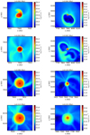 |
Fig. 1 Column density of run R2 at several snapshots and two scales. Left: box length is about 100 AU, right: box length is about 500 AU. |
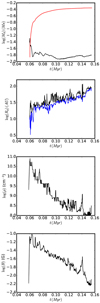 |
Fig. 2 Global properties of the disc of run R2 as a function of time. Top panel: disc mass (black line) and sink mass (red line). Second panel: disc radius (maximum radius: black line; mean radius: blue line, see Sect. 2.3). Third panel: mean gas density within the disc. Fourth panel: mean magnetic intensity of the disc. |
3.4 Structure of the magnetic field
The magnetic field is believed to play an important role in the disc by inducing transport of angular momentum through either magneto-rotational instability or magnetic braking and possibly by creating structures such as rings (Béthune et al. 2017; Suriano et al. 2018), therefore we look more closely into its structure.
The right panels of Fig. 3 show the value of βmag as a function of radius for several time steps as well as the mean radial profiles of Bz, Br, and Bϕ at three snapshots. The profiles of βmag reveal that while at early times the transition between βmag > 1 and βmag < 1 occurs through the shock, it is not the case at later times, where the disc outer part is significantly magnetised and presents βmag values < 1.
At time 0.086 Myr Bz and Bϕ have comparable amplitudes and dominate over Br. At times 0.134 and 0.153 Myr, Bz decreases and diffuses out of the disc while on the contrary the toroidal field grows in the disc outer part (i.e. between 20 AU and 100 AU). This growth of the toroidal field occurs in a region in which βmag < 1 and therefore where the field and the gas are well coupled. This is a natural consequence of the differential rotation (see for example Hennebelle & Teyssier 2008). As can be seen in the fourth left panel of Fig. 3, va is larger than Cs in the disc outer part. This excess of magnetic toroidal pressure leads to an inflated disc as observed in the third panel of Fig. B.1.
4 Influence of sink particles on disc evolution
To understand disc formation, it is necessary to use sink particles. How the sink particles are exactly implemented remains largely arbitrary and it is necessary to understand the effect of the sink algorithm on the disc properties.
4.1 Disc evolution without sink particle
To see the drastic influence of sink particles, the top panel of Fig. 4 portrays the column density of run R2ns in which no sink particle is being used. The comparison with Fig. 1 shows drastic differences. Clearly the disc is larger and presents prominent spiral patterns. These latter are largely a consequence of the fact that in the absence of sink particles, the gas that has accumulated in the central, thermally supported hydrostatic core may betransported back at larger radii and contribute to making the disc gravitationally unstable. Sink particles on the other hand introduce a strong irreversibility mimicking gas accretion onto stars. Clearly runs that do not use sinkparticles are not sufficiently realistic to describe the long time disc evolution. As we show below, the questions however of which sink parameters should be used and how the gas is retrieved from the grid are crucial.
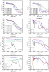 |
Fig. 3 Radial structure of the disc and surrounding envelope. Top left row: mean column density of the disc of run R2 as a function of radius. Second left panel: mean density of the disc vs. radius. Third and fourth left panels: various velocities vs. radius within the disc equatorial plane. Top right panel: βmag = Ptherm∕Pmag as a functionof radius within the disc for several time steps of run R2. Second, third, and fourth right panels: three snapshots, the mean radial, axial, and toroidal magnetic field as a function of radius. As can be seen while at early time, the axis field, Bz, is the dominant component, at later time the toroidal field dominates. |
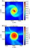 |
Fig. 4 Column density of run R2ns (top) and run R2hsink (bottom). These runs are identical to the reference run R2 but R2ns has no sink particle while R2hsink has a value nacc which is 4 times higher. They should be compared with Fig. 1. In the absence of sink particles the disc is more extended due to prominent spiral patterns. With a higher value of nacc the disc is also a bit bigger and more massive (see Fig. 5) than the disc in run R2. |
4.2 Influence of sink parameters on sink mass evolution
Top panel of Fig. 5 shows the sink mass (dashed lines) as a function of time for the numerically motivated runs (Table 1). In this series of runs, the numerical resolution varies by a factor 4 and the sink accretion threshold by a factor 40. Clearly, the sink mass evolution is only marginally influenced by the numerical parameters. In all runs the sinks formed roughly at the same time and the mass evolution is very similar.
This is an important conclusion because it confirms that the global evolution of the dense core is not very much affected by the numerical algorithm. In particular, the accretion rate onto the sink particles is likely a consequence of the large scale of the core rather than the detailed small-scale processes. In other words, the traditional picture that the infalling gas is stored in the centrifugally supported disc and then gets transported through it up to the star is not supported by the present simulations, at least in its simplest form.
4.3 Influence of sink parameters on disc evolution
To understand the influence of the sink parameter, we carried out run R2hsink, which has a value of nacc four times above that used in run R2. The bottom panel of Fig. 4 shows the disc of run R2hsink at time 0.08 Myr. As can be seen from a comparison with Fig. 1, the disc of run R2 and R2hsink are similar but the latter is more massive and slightly bigger. The reason is simply that the central disc density is higher for run R2hsink because of the higher value of nacc.
The top panel of Fig. 5 portrays the disc mass (solid lines) evolution, while bottom panel shows the disc radius for all runs listed in Table 1. Very large variations are observed. For instance the disc mass varies by more than one order of magnitude between runs R2lowr and runs R2r. This indicates that unlike for the sink mass, the disc mass and, to a lower extent, the disc radius very much depend on the numerical scheme. Below we analyse the various runs in detail, but two conclusions can already be drawn. First, the disc itself does not determine the accretion onto the star in the sense that varying the mass of the disc does not necessarily affect the accretion onto the star. Second, the disc properties, in particular its mass, cannot be reliably predicted because they are controlled by numerical parameters.
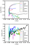 |
Fig. 5 Comparison between disc radius and mass for the 9 numerically motivated runs listed in Table 1. In top panelthe dashed lines represent the mass of the sink particles. While the sink mass does not depend significantly on the detailed of the numerical algorithm (i.e. sink threshold and resolution), the disc properties depend on it very much. |
4.3.1 Interdependence between resolution and sink particle threshold
First, we compare runs R2 and R2hsink. The only difference is the value of nacc, which is four times larger for R2hsink than for R2. The mass of the disc is about ≃3 times larger in run R2hsink while the disc radius is comparable though slightly larger. The reason is simply that as for run R2 (see Figs. 3 and A.1), the density within the sink particle is determined by nacc and since the profile is similar, the mass is almost proportional to nacc.
Second, we compare runs R2, R2lowr and R2r . These three runs have same value of nacc but differ in spatial resolution, which go from 2 AU (R2lowr) to 0.5 AU (R2r). The differences between the three discs are rather large, with a factor of ≃3–5 difference between the disc mass of runs R2lowr, R2, and R2r, respectively.In terms of radius, it is a factor of 2–3. This clearly indicates that both the resolution and sink density threshold, nacc, are important in determining the disc properties. This is confirmed by run R2lowrlsink, which has a resolution of 2 AU and a value nacc = 1012 cm−3, i.e. 10 times below the values inthe runs R2, R2lowr, and R2r . In this case, the disc mass is in between its value in runs R2 and R2r.
Roughly speaking the disc mass is proportional to dx−δnthres with δ ≃ 1−2. This can simply be understood as an inner boundary conditions. The density at the radius r = dx is equal to nacc = nthres∕3, therefore the density within the disc is about  with δ′≃ 1−1.5. Thus since the disc density decreases with increasing spatial resolution, the disc mass decreases as well.
4.3.2 Deciphering the role of density threshold and sink creation
To be certain that the effects we are observing are not due to differences of the sink creation time, we performed two runs, namely R2rr and R2rrhsink, for which we restart from an output of run R2. The two runs have a resolution of 0.5 AU and a threshold density of nacc = 1013 cm−3 and ten times this value respectively. We see that the disc mass of run R2rr drops by at least a factor of 3 while that of run R2rrhsink increases by about 50% while its radius does not evolve significantly. This confirms that the observed differences are due to the accretion condition onto the sink particles.
4.3.3 Amount of accreted gas
Finally, to investigate whether the disc mass is indeed influenced by the accretion rate from the disc onto the star, we performed run R2rlowacc, which is identical to run R2r except that the value of Cacc is 0.01 instead of 0.1. We recall that this is the fraction of gas above nthres, which is accreted at all time steps.
Figure 5 shows that the disc of run R2rlowacc is more massive (up to three to four times depending of the period) and roughly two times larger in radii. This confirms that the accretion rate at the inner boundary is a fundamental quantity that drastically impacts the disc properties, in particular its mass.
4.4 Physical interpretation
The results presented in Fig. 5 demonstrate that the accretion onto the sink particle, which operates as an inner boundary condition, is a major issue for the disc. Similar results are obtained by Machida et al. (2014), and recently by Vorobyov et al. (2019), who find that the accretion rate in their sink particles has a drastic impact on the disc. The obvious question is then whether the accretion scheme is realistic and what physically determines the inner boundary. We propose that the star-disc connection could be limiting the accretion and to illustrate how it may work we propose a simple model suggesting that the choices made are reasonable. We note that at the T Tauri stage, it is believed that the accretion proceeds through the magnetospheric accretion process (Bouvier et al. 2007). However our simulations take place far earlier than the T Tauri phase and also unlike what is assumed in the classical models, we do not find that most of the accretion proceeds through the bulk of the disc.
We use the classical stationary α-disc model which assumes that the effective disc viscosity is given by
 (2)
(2)
where h is the scale height, Ω is the Keplerian rotation, and α is a dimensionless number of the order of 10−3−10−2 depending on the disc physics. It is well known (e.g. Pringle 1981) that the disc surface density, Σ is given by
 (3)
(3)
where Ṁd is the accretion through the disc, M* is the mass of the central star, and C is a constant, which is usually chosen in such a way that at the star radius, R*, Σ(R*) = 0. This choice, while natural, leads to an infinite velocity at R* since
 (4)
(4)
and Ṁd is assumed to be constant through the disc.
To illustrate how the connection between the star and the disc, may influence the disc characteristics, we make very simple assumptions. First, we assume that the star is spherical and presents a profile of density, ρ*, temperature T*, and velocity v*. This latter is not zero because the star is accreting material from the outside at a rate Ṁ*, which we assume is nearly spherical. That is to say, the star is assumed to accrete both through the disc and also to receive a nearly spherical flux of gas. Since we are interested in the outer layer at which the disc connects, we have
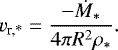 (5)
(5)
Since the fluid velocity and density must be continuous, we have vr,d = vr,* and ρd = ρ*, which leads to
 (6)
(6)
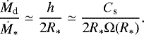
At early stage, the stellar radius is typically a few solar radii and the temperature of the gas on the verge to enter the star is about 104 K (Masunaga & Inutsuka 2000; Vaytet et al. 2018). We estimate
 (7)
(7)
which showsthat under these circumstances, the accretion rate through the disc is a few percent of the accretion onto the star. In the context of an α-disc, this also fixes the column density profile.
We stress that the present model is essentially illustrative and that a more detailed analysis should be performed. Other assumptionslead to different disc properties. This however supports the idea that the accretion rate through the disc and its density profile, at a large scale, may be influenced by the small-scale star-disc connection at the early stage of the star formation process. Unfortunately little is presently known on this phase as studies which have addressed the second collapse and the formation of the protostar itself (e.g. Machida et al. 2006; Tomida et al. 2013; Vaytet et al. 2018) are very limited in time owing to the small Courant conditions.
4.5 Criteria for sink accretion threshold
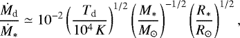
The obvious question is therefore what value of the accretion threshold should be used. As discussed in the previous section, this is not an easy question as it may request a detailed knowledge of the disc structure at small radii may be up to the star itself. To proceed we again use the standard α-disc model. Using Eqs. (2) and (3) we get
 (8)
(8)
Now with Eq. (1), we have when n ≫ nAD :
 (9)
(9)
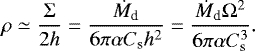
where  is the sound speed in the isothermal envelope and is about 0.2 km s−1 and this leads the gas density to
 (10)
(10)
where mp is the mean mass per particle and n = ρ∕mp. We therefore obtain
 (11)
(11)
Several points must be discussed. First the typical value of n at 1 AU is expected to be around 1013 cm−3 if M* = 0.3 M⊙ as is the case in the present study. Second this density depends on the accretion rate through the disc as well as the effective viscosity. Both are heavily uncertain and their estimate requires a careful and specific investigation. The reference value Ṁd = 10−7 M⊙ yr−1 is simply based on Eq. (7) and on the measured accretion ratio in the sink, which is of the order of 10−6− 10−5 M⊙ yr−1.
When using the sink particles, we must make sure that the density at which the gas is accreted within the sink is close to the value stated by Eq. (11). There is however another source of uncertainty which comes from the radius at which this should be evaluated. Typically, it could be either the sink radius, 4d x, or the resolution, d x. As revealed by Fig. 3, the density reached nacc only in the very centre. Therefore estimating nacc at d x seems to be a better choice. In any case, there is, as described in the present section, a dependence of the accretion threshold nacc into the resolution. Typically from Eq. (11), this quantity broadly scales as d x−2, which is compatible with what as been inferred from the numerical experiments presented above. Finally, we stress that in reality the value of nacc should be time dependent as it depends on M* and Ṁd, which both evolve with time. It is also possibly physics dependent since it depends on α, which in turn may depend on the magnetic intensity for instance.
5 Influence of initial conditions on disc formation and evolution
We now investigate the influence that initial conditions have on the disc evolution. We focus on the global disc properties, i.e. its mass and size. As discussed in the previous section, the accretion threshold nacc is of primary importance while highly uncertain. We adopt the value nacc = 1013 cm−3 as it is close to our analytical estimate. While it is likely that better, time-dependent estimates will have to be used in the future, it is nevertheless important to investigate the influence of initial conditions because they also play an important role in disc evolution. In particular, the resulting discs can be compared to understand the consequences of the various processes. From the previous section, we saw that the mass of the disc is nearly proportional to nacc, as long as this parameter varies from a factor of a few. So in principle, the results presented below should remain valid for other values of nacc by simply multiplying the disc mass by nacc∕1013 cm−3.
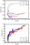 |
Fig. 6 Comparison between disc mass and radius for runs R1, R2 R10, i.e. having 3 levels of rotation corresponding to βrot = 0.01, 0.04, and 0.0025, respectively. |
5.1 Impact of rotation
Figure 6 shows the disc mass and disc radius as a function of time for runs R1, R2, and R10 (i.e. βrot = 0.01, 0.04, and 0.0025 respectively). During the first 50 kyr, there is a clear trend for the disc of run R1 to be about two times less massive on average that the disc of run R2 but at time ≃0.11 Myr, the two runs present discs of comparable masses. The radius of the two discs are close but there is a clear trend for the disc of run R1 to be slightly smaller by a few tens of percents. With run R10 the situation is a bit more confusing. There is a short phase, between 0.07 and 0.08 Myr during which the disc of run R10 is about 50% smaller and less massive than the disc of run R1. However, past this phase, the disc of run R10 becomes even slightly bigger and more massive than the disc of run R2. A more detailed analysis reveals that the disc in run R10 becomes very elliptical. Altogether rotation appears to have only a modest influence on the disc characteristics, although obviously very small rotation would certainly lead to major differences.
At first sight this is surprising since the disc radius is proportional to j2, where j is the angular momentum. Therefore increasing βrot by a factor of 4 may lead to a disc that is four times bigger. This however is not the case because magnetic braking largely controls the formation of disc and is responsible for redistributing the angular momentum through the core. Indeed the analytical expression of the disc radius (Eq. (13) of Hennebelle et al. 2016) does not entail any dependence on βrot (contrarily to Eq. (14) of Hennebelle et al. 2016). This is a consequence of magnetic braking and magnetic field generation. A larger rotation leads to a stronger Bϕ, which in turn leads to more efficient magnetic braking.
For the long term evolution, in particular after symmetry breaking takes place, the reason of the mass similarity may be due to the sink motion with respect to the collapsing gas and a consequence of the inertia forces (see Verliat et al. 2020)
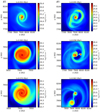 |
Fig. 7 Column density of runs R3 (left) and R5 (right), i.e. weakly magnetised runs, for two snapshots. For run R3 even though the magnetic intensity is 3 times weaker than for run R2, the disc is only marginally larger. Two noticeable differences however are that the disc presents strong and persistent spiral arms and that there remains large-scale spiral arms outside the disc. As can be seen, run R5 (which has a magnetic intensity about 4 times lower than run R2) fragments in 2 objects. |
5.2 Impact of magnetic intensity
The magnetic intensity is expected to be a fundamental parameter regarding disc formation and in this section we investigate four values of μ, going from significantly magnetised (i.e. μ−1 = 0.3) to weakly magnetised (μ−1 = 0.07). Figure 7 shows the disc at three snapshots for runs R3 (left, μ−1 = 0.1) and R5 (right, μ−1≃ 0.07). The disc in run R3 is a bit larger than the disc of run R2 and is surrounded by spiral arms whose size is about 200–400 AU, which persist and even grow with time (not shown here for conciseness). There are also prominent spiral arms within the disc itself as shown by the middle and bottom left panel. This is very similar to the disc shown by Tomida et al. (2017).
The disc formed early in run R5 (top right panel) is visibly both massive and large with prominent spiral arms. Further fragments develop through gravitational instability within the arms and a new object forms as seen in bottom right panel. Two smaller discs form around each of the two stars with radii of the order of 20–40 AU. Around the binary a larger scale rotating structure is seen, which may give raise to a circumbinary disc.
Figure 8 portrays the disc mass and disc radius as a function of time for runs R2, R3, and R4 (μ−1 = 0.3, 0.1, and 0.15, respectively,but not run R5 since it fragments). First we note that the sinks form about 10 kyr later in run R2 than in runs R3 and R4 because of the magnetic support which delays the collapse by about 25% in time. The disc in run R3 is about five to six times more massive than the disc of run R2 and it is about two times larger; the large fluctuations are due to the spiral arms which continuously evolve. The disc of run R4 is initially a little more massive than that in run R2 but over time t = 0.08 Myr, the mass of the discs of runs R2 and R4 are almost identical. In terms of radius, the difference is of the order of ≃50% until t = 0.09 Myr, where the two radii become very close.
Altogether these results show that for magnetic fields such that μ−1 > 0.15, the magnetic intensity does not influence very strongly the disc properties. For weaker field, typically corresponding to μ−1 = 0.07−0.1, we see a stronger dependence leading to bigger discs that can possibly fragment. As explained in Hennebelle et al. (2016) this is largely a consequence of the ambipolar diffusion that tends to regulate the magnetic intensity at high density. We note that more variability is reported in Masson et al. (2016) than what is inferred in this work particularly regarding the cases μ = 3 and μ ≃ 6. The difference comes from the sink particles, which are not used in Masson et al. (2016). As shown in Fig. 4, when they are not used strong spiral patterns develop because the gas that piles up in the centre can expand back, thereby forming more massive disc than it should.
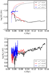 |
Fig. 8 Comparison between disc mass and radius for runs R2, R3, and R4, i.e. having 3 levels of magnetisation corresponding to μ−1 = 0.3, 0.1, and 0.15, respectively. |
5.3 Impact of misalignment
Misalignment has been identified to play a significant role in the process of disc formation particularly for values of μ >5 (Hennebelle & Ciardi 2009; Joos et al. 2012; Li et al. 2013; Gray et al. 2018; Hirano & Machida 2019). Typically it has been found that large discs form more easily in the perpendicular configuration, although Tsukamoto et al. (2018) conclude based on an analysis of the amount of angular momentum that this may not be the case when non-ideal MHD is considered. This is however based on the amount of angular momentum available in the dense gas as these authors do not report about the discs themselves.
Figure 9 shows the disc for runs R7 (left panels) and R9 (right panels), which both have an initial angle between magnetic and rotation axis equal to 90° and a magnetisation of μ−1 = 0.3 and μ−1= 0.1, respectively. Both discs have their axis along the x-axis i.e. along the initial rotation axis.
The discof run R7 is small in size and comparable to that of run R2. This is confirmed by Fig. 10, which shows that both the mass and radius are very similar to those of run R2, where the radius of the latter is a few tens of percent smaller than the former.
The case of larger μ, i.e. runs R3 and R9 is different. From Fig. 9, it is clear that the disc of run R9 is rather large and typically three times larger than the disc of run R3. This is also clearly shown by Fig. 10, where it is seen that at the end of the integration; both the mass and radius of run R9 disc are almost three times those of run R3 disc. While the disc in run R9 is both massive and large, it does not seem to show any sign of fragmentation so far. The reason is likely because it has a stronger field than run R5 for instance.
The conclusion is therefore broadly similar to that inferred from ideal MHD calculations (Joos et al. 2012), that is to say the orientation does not have a drastic impact for a moderate to strong field (i.e. μ < 3); it can make a significant difference for weak magnetisation (in the present case μ = 10). We note nevertheless that in ideal MHD calculations, the influence of the misalignment appears to be important for values as low as μ = 3.
5.4 Impact of turbulence
The impact of turbulence on disc formation has been studied in the context of ideal MHD and it has been found (Santos-Lima et al. 2012; Joos et al. 2013) that it reduces the magnetic flux in the core inner part therefore favouring disc formation. It has also been proposed (Seifried et al. 2013) that the disorganised structure of the field, induced by turbulence, reduces the effect of magnetic braking, while Gray et al. (2018) conclude that the most important effect of turbulence is the misalignment it induces (see also Joos et al. 2013).
Cases that included both turbulence and ambipolar diffusion are presented in Hennebelle et al. (2016) and it has been found that the discs were not particularly different from the cases in which no turbulence was initially present. Both runs R6 and R8 (which are identical apart from their magnetisation) confirm this conclusion as revealed by Fig. 11, in which the disc and radius mass are portrayed for runs R2 (μ−1 = 0.3 and no turbulence) and R6 (μ−1 = 0.3 with an rms Mach number of 1 initially) as well as runs R4 (μ−1 = 0.15 and no turbulence) and R8 (μ−1 = 0.15 with an rms Mach number of 1 initially). Atearly time, disc of run R6 is 50% smaller than for R2 but this may be in part due to the slightly delayed collapse of run R6 with respect to run R2 (a consequence of turbulence) and also to the lower rotation of run R6. After 20 kyr, the discs of runs R2 and R6 have indistinguishable sizes and masses.
We conclude that in the presence of ambipolar diffusion, turbulence does not have a significant impact on the disc. This is likely because ambipolar diffusion has an effect on the magnetic field that dominates over the diffusion induced by turbulence. Another complementary effect is the dissipative nature of ambipolar diffusion, which likely tends to reduce turbulence by enhancing its dissipation.
5.5 Magnetic intensity versus density
To interpret the results inferred in this section, the magnetic intensity distribution is of fundamental importance since magnetic braking is largely controlling disc formation. Figure 12 portrays the mean magnetic intensity, B, per logarithmic bin of densities for all runs at time 0.06 Myr. We note that the magnetic field intensity as a function of density does not evolve very significantly with time so the particular choice made in this work is not consequential.
In the envelope for densities between 104 and 108 cm−3, B increases with the density. Some discrepancies are seen between the runs. The most magnetised runs present a more shallow profiles (typically with power-law exponents of about one-half) while for the less magnetised ones, the profiles are stiffer (and more compatible with power-law exponents close to two-thirds). At higher densities, i.e. 108 –1010 cm−3 dependingon the runs, a plateau of magnetic intensities formed. Its value is nearly the same for all runs, except for runs R3, R5, and R9, which present lower intensities. The reason for this behaviour (see Hennebelle et al. 2016) is that the ideal MHD holds in the low-density envelope while at high density, ambipolar diffusion is dominant and an equilibrium settles between the inwards flux of magnetic field dragged by the collapsing motion and ambipolar diffusion.
The distribution for run R9 is particularly intriguing. It has the same initial magnetisation as run R3, which is more magnetised than run R5, but the magnetisation at high density in run R9 is the weakest. On the other hand, we see that it presents an excess compared to the other runs of magnetic intensity around n ≃106 cm−3. This strongly suggests that in run R9 efficient diffusion of the magnetic field occurred. This is probably a consequence of the perpendicular configuration and weak intensity which lead to a strongly wrapped field. Importantly, we find an obvious qualitative correlation between the size of the disc and the field intensity in the core inner part (i.e. n > 108 cm−3).
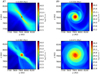 |
Fig. 9 Column density of runs R7 (left) and R9 (right) for two snapshots. Both runs present an initial misalignment between the magnetic and rotation axis of 90°. Run R7, which is has the same magnetic intensity as run R2, presents a disc that is rather similar to it. Run R9, which is 3 times less magnetised than run R2 (and has the same magnetisation as run R3), presents a massive and large disc. |
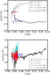 |
Fig. 10 Comparison between disc radius and mass for runs R2, R3, R7, and R9, i.e. having 2 levels of magnetisation corresponding to μ−1 = 0.3 and 0.1 as well as two angles between the rotation and magnetic field axis initially, namely 30° and 90°. |
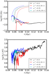 |
Fig. 11 Comparison between disc radius and mass for runs R2, R4, R6, and R8, i.e. having 2 levels of magnetisation corresponding to μ−1 = 0.3 and 0.15 as well as two values of initial turbulent Mach number initially, namely 0 and 1. |
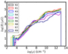 |
Fig. 12 Mean magnetic intensity as a function of density within the 9 runs. Apart from runs R3, R5, and R9, which all have μ−1 < 0.1, i.e. a very low field initially, the distribution of the magnetic intensity is remarkably similar for all runs. |
5.6 Comparison between simulation and analytical theory of disc radii
To better understand the physics that governs disc evolution, we now compare the numerical results presented above with the analytical modelling presented in Hennebelle et al. (2016). We note that this expression is obtained by simply requiring the equality between on one hand the magnetic braking and rotation time and on the other hand, the magnetic diffusion and generation of the toroidal magnetic field at the disc edge. The radius expression is
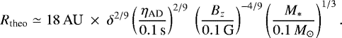 (12)
(12)
In this expression, ηAD is the magnetic resistivity, Bz is the vertical component of the magnetic field at the edge of the disc, and M* the mass of the star. The quantity δ is a coefficient such that 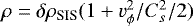 , where ρSIS is the density of the singular isothermal sphere. We note that while this expression is reasonable to describe the equatorial density of a rotating hydrodynamical collapsing core, it is not obviously the case in a misaligned magnetised dense core as the densest part of the collapsing envelope, the pseudo-disc, generally does not lie in the plane of the disc (as is particularly obvious from Figs. B.1 and B.2). Moreover as it is clear from Fig. 3, the envelope and the disc are connected through a shock. This suggests that using the expression
 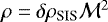 for the density at the disc edge would be more appropriate. However, since
 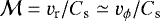 , this leads to exactly the same dependence and leaves Eq. (12) essentially unchanged.
To test this formula, we measured the mean magnetic intensity in the disc as a function of time. This gives a reasonable proxy for the magnetic field at the edge. The values of ηAD and δ are not easy to estimate because the density changes abruptly at the edge of the disc. Fortunately, ηAD in this range of parameter does not change too steeply and both parameters come with an exponent 2∕9 in Eq. (12). For the sake of simplicity, we therefore keep these parameters constant.
Figure 13 shows the ratio of the measured disc radius to the theoretical expression for the eight runs (run R5 is not considered because it fragments) as a function of time. Altogether we see that within a factor of ≃ 2, we indeed have Rd ≃ Rtheo. Apart from run R9 and maybe R3, there is a general trend for Rtheo to be about 50% larger, which is probably a consequence of ηAD ≃ 0.1 to be a little too high and more generally to the difficulty in inferring a single value of Bz and of η. For most runs, apart from the large fluctuations at the beginning where the disc is not well settled, R∕Rtheo varies within a factor of about 2. This is similar to what has been inferred in Hennebelle et al. (2016), although since sink particles are used, the agreement is even better. Compared with the disc radius as a function of time and for different runs (see for instance Fig. 10), it is clear that the radio Rd∕Rtheo presents much less variability which also illustrates the reasonable validity of Eq. (12). In particular, we see that Rd ∕Rtheo does not vary appreciably with time, which indicates that Rd ∝ M1∕3 is a good approximation. We conclude that altogether the theoretical expression provides the correct answer within a factor of ≃2–3.
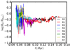 |
Fig. 13 Ratio of disc radius and theoretical prediction from Hennebelle et al. (2016) for runs R1–R9. The analytical model leads to reasonable agreement with the simulations within a factor of about 2. |
6 Conclusions
In this paper we present two series of numerical simulations aimed to describe the collapse of a magnetised dense core in which non-ideal MHD, namely the ambipolar diffusion, operates. The first series of runs explore the influence of the numerical parameters such as the numerical resolution and sink particle accretion scheme. The goal of the second series of runs is to understand the impact of initial conditions on the disc properties. In particular, we vary the initial magnetic intensity, rotation speed, inclination of the field with respect to the rotation axis, and level of turbulence.
We found that while the mass of the central object is insensitive to the numerical scheme, the disc mass on the contrary depends significantly on the accretion scheme onto the sink particle. Essentially at a given spatial resolution, the disc density increases with nacc, the density above which the sink would accrete. This in particular implies that the disc mass increases with nacc. For a given value of nacc, the disc mass decreases if the resolution increases. This is because the sink particles act as an inner boundary and what matters is the density imposed at this boundary. We suggest that, in reality, the disc density profile and therefore its mass distribution are determined by small-scale accretion (and perhaps star-disc interaction) together with disc transport properties.
Exploring a large sets of initial conditions, we found that the most critical parameter is the magnetic intensity particularly when it becomes small, i.e. for μ−1 < 0.1, for which the disc radius increases with μ. For μ−1 < 0.07, we found that the disc fragments, leading to a binary. For magnetisation larger than μ−1> 0.15 the disc properties do not change strongly with magnetisation. By changing the rotation speed from βrot = 0.01 to βrot = 0.04, we found that at least in this range of parameter, the size of the disc is not significantly modified for instance. The reason for this somewhat counter-intuitive result is that magnetic braking really controls the process of disc formation and more rotation also leads to a larger toroidal field and more braking. The misalignment between the rotationaxis and magnetic field direction is found to play a minor role when the field is substantial (μ−1 = 0.3), but has a major impact when the field is weak (μ−1 = 0.1) in which case a large disc of about 100 AU in radius forms. Finally, two runs include turbulence. They present discs which are nearly identical to the discs formed in the absence of turbulence.
We conclude that the disc physical characteristics, and in particular its mass, are to a large extent determined by the local physical processes that is to say the collapse, magnetic braking, field diffusion, and an inner boundary condition possibly determined by star-disc interaction. We only find the resulting discs present significantly different properties when the magnetic field is relatively weak, i.e. μ−1 < 0.15.
The standard disc that forms in our simulations has a mass of about 10−2 M⊙ (which we stress depends on the accretion condition onto the central sink), a radius of 20–30 AU, and is weakly magnetised in the inner part (βmag > 100) and strongly magnetised in the outer part (βmag < 0.1). At later time, as the envelope disappears, the inner part of the disc remains barely changed by the external part as the disc develops. This is characterised by a weaker βmag and a stiff density profile, which we estimate to be broadly ∝r−4.
Acknowledgements
We thank the anonymous referee for a detailed and helpful report which has improved the paper. This work was granted access to HPC resources of CINES and CCRT under the allocation x2014047023 made by GENCI (Grand Equipement National de Calcul Intensif). This research has received funding from the European Research Council under the European Community’s Seventh Framework Programme (FP7/2007-2013 Grant Agreement no. 306483). Y.-N. Lee acknowledges the financial support of the UnivEarthS Labex program at Sorbonne Paris Cité (ANR-10-LABX-0023 and ANR-11-IDEX-0005-02). We thank the programme national de physique stellaire, the programme national de planétologie and the programme national de physique et chimie du milieu interstellaire for their supports.
Appendix A Disc profiles for runs R 2hsink and R3
In this section we give more detail on two of the runs, namely Run2hsink and R3, which we recall differ from our reference run R2 by a higher value of nthres (i.e. the value at which the sink accretes) and a weaker magnetisation. The two discs are larger than the disc of R2 and also more massive (Figs. 5 and 8).
Figures A.1 and A.2 show the column density, the density in the equatorial plan, and the βmag as a function of radius for several time steps. These figures also show several velocities at a given snapshot. These plots can be compared with Fig. 3.
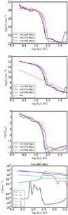 |
Fig. A.1 Radial structure of the disc of run R2hsink (i.e. nthres = 1.2 1014 cm−3). Top row: mean column density of the disc as a function of radius. Second panel: mean density of the disc vs radius. Third panel: βmag = Ptherm∕Pmag as a function of radius. Fourth panel: various velocities vs. radius within the disc equatorial plane. |
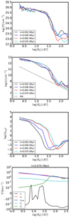 |
Fig. A.2 Radial structure of the disc of run R3 (i.e. μ−1 = 0.1). Top row: mean column density of the disc as a function of radius. Second panel: mean density of the disc vs. radius. Third panel: βmag = Ptherm∕Pmag as a function of radius. Fourth panel: various velocities vs. radius within the disc equatorial plane. |
For run R2hsink, the most important difference comes from the central density that is three to four times higher, which is a direct consequence of the higher value of nthres. The value of βmag is also slightly higher because of higher density. For run R3, the mean density profile is not very different from R2 (the spiral structure is not seen on the 1D profile). The value of βmag is about two to four times lower. Apart from these differences, the other profiles tend to be remarkably similar.
Appendix B Outflows
As is the case in most MHD collapse calculations (e.g. Banerjee & Pudritz 2006; Machida et al. 2006; Ciardi & Hennebelle 2010; Tomida et al. 2010; Hirano & Machida 2019), prominent outflows due to the magneto-centrifugal mechanism (Frank et al. 2014) also develop in the present simulations and for the sake of completeness we present them in this appendix.
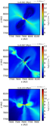 |
Fig. B.1 Density and velocity field at three snapshots for run R2. |
B.1 Outflow qualitative description
Figure B.1 portrays density slices on which the velocity field is overplotted at three different snapshots. From the top and middle panels, we see that a magnetised cavity with expanding motion starts developing early. Indeed the corresponding time is very close to the moment at which the sink particle is being introduced in run R2. Interestingly the gas close to the sink and disc is infalling and it only expands at a distance of a few tens of astronomical units. The cavity is broadly aligned with the direction of the mean magnetic field. The bottom panel shows that the outflow persists at later time and becomes relatively faster. The cavities are asymmetrical and do not occupy the whole disc surface as accretion along the disc axis is still occurring.
Figure B.2 is identical to Fig. B.1 but shows run R3 (which has μ−1= 0.1). The top panel shows again that the outflow starts early and is concomitant to the sink creation. Again the velocity close to the disc and sink reveals that the gas is infalling. The middle panel shows that the cavities develop in a rather symmetric way and occupy all the surface within and above the disc. The bottom panel shows a larger scale view about 10 kyr later. The outflow stays symmetrical and well collimated.
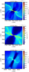 |
Fig. B.2 Density and velocity field at three snapshots for run R3. |
B.2 Outflow velocity and mass
To quantify further the outflows in our simulations, we selected all computational cells which have a radial velocity that is positive (therefore expanding) and larger than 1 km s−1 . Figure B.3 represents the total mass within the flow as well as its maximum velocity for all the runs listed in Table 2 except for run R9, which does not present outflow. The total mass remains below 1% of the sink mass, except initially when the sink has a low mass. It should be stressed however that after a few thousand years, the outflows reach the boundary of the computational domain and therefore the mass is not properly counted. The velocity threshold used to define the flow is obviously critical. Choosing smaller values, obviously leads to higher estimate but there is then a confusion with the expanding envelope which surrounds the core since the medium outside the core initially has low pressure. The largest velocity within the flow tends to be similar in all runs and goes from about 5 km s−1 at early times to 15 km s−1 at later times.
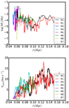 |
Fig. B.3 Top and bottom panels: mass within and largest velocity of the outflow defined as gas having a positive radial velocity larger than 1 km s−1 for all runs (except run R9 which presents no outflow). |
References
- Allen, A., Li, Z.-Y., & Shu, F. H. 2003, ApJ, 599, 363 [NASA ADS] [CrossRef] [Google Scholar]
- Banerjee, R., & Pudritz, R. E. 2006, ApJ, 641, 949 [NASA ADS] [CrossRef] [Google Scholar]
- Béthune, W., Lesur, G., & Ferreira, J. 2017, A&A, 600, A75 [NASA ADS] [CrossRef] [EDP Sciences] [Google Scholar]
- Bleuler, A., & Teyssier, R. 2014, MNRAS, 445, 4015 [NASA ADS] [CrossRef] [Google Scholar]
- Bouvier, J., Alencar, S. H. P., Harries, T. J., Johns-Krull, C. M., & Romanova, M. M. 2007, in Protostars and Planets V, eds. B. Reipurth, D. Jewitt, & K. Keil (Tucson: University of Arizona Press), 479 [Google Scholar]
- Ciardi, A., & Hennebelle, P. 2010, MNRAS, 409, L39 [NASA ADS] [Google Scholar]
- Dapp, W. B., & Basu, S. 2010, A&A, 521, L56 [NASA ADS] [CrossRef] [EDP Sciences] [Google Scholar]
- Dapp, W. B., Basu, S., & Kunz, M. W. 2012, A&A, 541, A35 [NASA ADS] [CrossRef] [EDP Sciences] [Google Scholar]
- Dutrey, A., Semenov, D., Chapillon, E., et al. 2014, in Protostars and Planets VI, eds. H. Beuther, R. S. Klessen, C. P. Dullemond, & T. Henning (Tucson: University of Arizona Press), 317 [Google Scholar]
- Frank, A., Ray, T. P., Cabrit, S., et al. 2014, in Protostars and Planets VI, eds. H. Beuther, R. S. Klessen, C. P. Dullemond, & T. Henning (Tucson: University of Arizona Press), 451 [Google Scholar]
- Fromang, S., Hennebelle, P., & Teyssier, R. 2006, A&A, 457, 371 [NASA ADS] [CrossRef] [EDP Sciences] [Google Scholar]
- Galli, D., Lizano, S., Shu, F. H., & Allen, A. 2006, ApJ, 647, 374 [NASA ADS] [CrossRef] [Google Scholar]
- Gray, W. J., McKee, C. F., & Klein, R. I. 2018, MNRAS, 473, 2124 [NASA ADS] [CrossRef] [Google Scholar]
- Greaves, J. S., & Rice, W. K. M. 2010, MNRAS, 407, 1981 [NASA ADS] [CrossRef] [Google Scholar]
- Hennebelle, P., & Ciardi, A. 2009, A&A, 506, L29 [NASA ADS] [CrossRef] [EDP Sciences] [Google Scholar]
- Hennebelle, P., & Fromang, S. 2008, A&A, 477, 9 [NASA ADS] [CrossRef] [EDP Sciences] [Google Scholar]
- Hennebelle, P., & Inutsuka, S.-i. 2019, Front. Astron. Space Sci., 6, 5 [NASA ADS] [CrossRef] [Google Scholar]
- Hennebelle, P., & Teyssier, R. 2008, A&A, 477, 25 [NASA ADS] [CrossRef] [EDP Sciences] [Google Scholar]
- Hennebelle, P., Commerçon, B., Chabrier, G., & Marchand, P. 2016, ApJ, 830, L8 [NASA ADS] [CrossRef] [Google Scholar]
- Hirano, S., & Machida, M. N. 2019, MNRAS, 485, 4667 [NASA ADS] [CrossRef] [Google Scholar]
- Inutsuka, S.-i. 2012, Prog. Theor. Exp. Phys., 2012, 01A307 [Google Scholar]
- Joos, M., Hennebelle, P., & Ciardi, A. 2012, A&A, 543, A128 [NASA ADS] [CrossRef] [EDP Sciences] [Google Scholar]
- Joos, M., Hennebelle, P., Ciardi, A., & Fromang, S. 2013, A&A, 554, A17 [NASA ADS] [CrossRef] [EDP Sciences] [Google Scholar]
- Jørgensen, J. K., van Dishoeck, E. F., Visser, R., et al. 2009, A&A, 507, 861 [NASA ADS] [CrossRef] [EDP Sciences] [Google Scholar]
- Krasnopolsky, R., Li, Z.-Y., Shang, H., & Zhao, B. 2012, ApJ, 757, 77 [CrossRef] [Google Scholar]
- Li, Z.-Y., Krasnopolsky, R., & Shang, H. 2013, ApJ, 774, 82 [NASA ADS] [CrossRef] [Google Scholar]
- Li, Z. Y., Banerjee, R., Pudritz, R. E., et al. 2014, in Protostars and Planets VI, eds. H. Beuther, R. S. Klessen, C. P. Dullemond, & T. Henning (Tucson: University of Arizona Press), 173 [Google Scholar]
- Machida, M. N., Inutsuka, S.-i., & Matsumoto, T. 2006, ApJ, 647, L151 [NASA ADS] [CrossRef] [Google Scholar]
- Machida, M. N., Inutsuka, S.-i., & Matsumoto, T. 2014, MNRAS, 438, 2278 [NASA ADS] [CrossRef] [Google Scholar]
- Machida, M. N., Matsumoto, T., & Inutsuka, S.-i. 2016, MNRAS, 463, 4246 [Google Scholar]
- Manara, C. F., Morbidelli, A., & Guillot, T. 2018, A&A, 618, L3 [NASA ADS] [CrossRef] [EDP Sciences] [Google Scholar]
- Marchand, P., Masson, J., Chabrier, G., et al. 2016, A&A, 592, A18 [NASA ADS] [CrossRef] [EDP Sciences] [Google Scholar]
- Marchand, P., Commerçon, B., & Chabrier, G. 2018, A&A, 619, A37 [NASA ADS] [CrossRef] [EDP Sciences] [Google Scholar]
- Masson, J., Teyssier, R., Mulet-Marquis, C., Hennebelle, P., & Chabrier, G. 2012, ApJS, 201, 24 [NASA ADS] [CrossRef] [Google Scholar]
- Masson, J., Chabrier, G., Hennebelle, P., Vaytet, N., & Commerçon, B. 2016, A&A, 587, A32 [NASA ADS] [CrossRef] [EDP Sciences] [Google Scholar]
- Masunaga, H.,& Inutsuka, S.-i. 2000, ApJ, 531, 350 [NASA ADS] [CrossRef] [Google Scholar]
- Masunaga, H., Miyama, S. M., & Inutsuka, S.-i. 1998, ApJ, 495, 346 [Google Scholar]
- Maury, A. J., André, P., Hennebelle, P., et al. 2010, A&A, 512, A40 [NASA ADS] [CrossRef] [EDP Sciences] [Google Scholar]
- Maury, A. J., André, P., Testi, L., et al. 2019, A&A, 621, A76 [NASA ADS] [CrossRef] [EDP Sciences] [Google Scholar]
- Mouschovias, T. C., & Spitzer, L., J. 1976, ApJ, 210, 326 [NASA ADS] [CrossRef] [Google Scholar]
- Murillo, N. M., Lai, S.-P., Bruderer, S., Harsono, D., & van Dishoeck, E. F. 2013, A&A, 560, A103 [NASA ADS] [CrossRef] [EDP Sciences] [Google Scholar]
- Najita, J. R., & Kenyon, S. J. 2014, MNRAS, 445, 3315 [NASA ADS] [CrossRef] [Google Scholar]
- Ohashi, N., Saigo, K., Aso, Y., et al. 2014, ApJ, 796, 131 [NASA ADS] [CrossRef] [Google Scholar]
- Padovani, M., Hennebelle, P., & Galli, D. 2013, A&A, 560, A114 [NASA ADS] [CrossRef] [EDP Sciences] [Google Scholar]
- Price, D. J., & Bate, M. R. 2007, MNRAS, 377, 77 [NASA ADS] [CrossRef] [Google Scholar]
- Pringle, J. E. 1981, ARA&A, 19, 137 [NASA ADS] [CrossRef] [Google Scholar]
- Santos-Lima, R., de Gouveia Dal, E. M., & Lazarian, A. 2012, ApJ, 747, 21 [NASA ADS] [CrossRef] [Google Scholar]
- Seifried, D., Banerjee, R., Pudritz, R. E., & Klessen, R. S. 2013, MNRAS, 432, 3320 [NASA ADS] [CrossRef] [Google Scholar]
- Shu, F. H. 1977, ApJ, 214, 488 [NASA ADS] [CrossRef] [Google Scholar]
- Suriano, S. S., Li, Z.-Y., Krasnopolsky, R., & Shang, H. 2018, MNRAS, 477, 1239 [NASA ADS] [CrossRef] [Google Scholar]
- Testi, L., Birnstiel, T., Ricci, L., et al. 2014, in Protostars and Planets VI, eds. H. Beuther, R. S. Klessen, C. P. Dullemond, & T. Henning (Tucson: University of Arizona Press), 339 [Google Scholar]
- Teyssier, R. 2002, A&A, 385, 337 [NASA ADS] [CrossRef] [EDP Sciences] [Google Scholar]
- Tobin, J. J., Looney, L. W., Li, Z.-Y., et al. 2016, ApJ, 818, 73 [NASA ADS] [CrossRef] [Google Scholar]
- Tomida, K., Tomisaka, K., Matsumoto, T., et al. 2010, ApJ, 714, L58 [NASA ADS] [CrossRef] [Google Scholar]
- Tomida, K., Tomisaka, K., Matsumoto, T., et al. 2013, ApJ, 763, 6 [NASA ADS] [CrossRef] [Google Scholar]
- Tomida, K., Machida, M. N., Hosokawa, T., Sakurai, Y., & Lin, C. H. 2017, ApJ, 835, L11 [NASA ADS] [CrossRef] [Google Scholar]
- Tsukamoto, Y., Okuzumi, S., Iwasaki, K., Machida, M. N., & Inutsuka, S.-i. 2017, PASJ, 69, 95 [CrossRef] [Google Scholar]
- Tsukamoto, Y., Okuzumi, S., Iwasaki, K., Machida, M. N., & Inutsuka, S. 2018, ApJ, 868, 22 [NASA ADS] [CrossRef] [Google Scholar]
- Vaytet, N., Commerçon, B., Masson, J., González, M., & Chabrier, G. 2018, A&A, 615, A5 [NASA ADS] [CrossRef] [EDP Sciences] [Google Scholar]
- Verliat, A., Hennebelle, P., Maury, A. J., & Gaudel, M. 2020, A&A, in press, https://doi.org/10.1051/0004-6361/201936394 [Google Scholar]
- Vorobyov, E. I., Skliarevskii, A. M., Elbakyan, V. G., et al. 2019, A&A, 627, A154 [NASA ADS] [CrossRef] [EDP Sciences] [Google Scholar]
- Wurster, J., & Bate, M. R. 2019, MNRAS, 486, 2587 [NASA ADS] [Google Scholar]
- Wurster, J., & Li, Z.-Y. 2018, Front. Astron. Space Sci., 5, 39 [NASA ADS] [CrossRef] [Google Scholar]
- Wurster, J., Price, D. J., & Bate, M. R. 2016, MNRAS, 457, 1037 [NASA ADS] [CrossRef] [Google Scholar]
- Wurster, J., Bate, M. R., & Price, D. J. 2018, MNRAS, 476, 2063 [NASA ADS] [CrossRef] [Google Scholar]
- Wurster, J., Bate, M. R., & Price, D. J. 2019, MNRAS, 489, 1719 [NASA ADS] [CrossRef] [Google Scholar]
- Zhao, B., Caselli, P., Li, Z.-Y., et al. 2016, MNRAS, 460, 2050 [NASA ADS] [CrossRef] [Google Scholar]
- Zhao, B., Caselli, P., Li, Z.-Y., & Krasnopolsky, R. 2018, MNRAS, 473, 4868 [NASA ADS] [CrossRef] [Google Scholar]
All Tables
All Figures
|
Fig. 1 Column density of run R2 at several snapshots and two scales. Left: box length is about 100 AU, right: box length is about 500 AU. |
| In the text | |
|
Fig. 2 Global properties of the disc of run R2 as a function of time. Top panel: disc mass (black line) and sink mass (red line). Second panel: disc radius (maximum radius: black line; mean radius: blue line, see Sect. 2.3). Third panel: mean gas density within the disc. Fourth panel: mean magnetic intensity of the disc. |
| In the text | |
|
Fig. 3 Radial structure of the disc and surrounding envelope. Top left row: mean column density of the disc of run R2 as a function of radius. Second left panel: mean density of the disc vs. radius. Third and fourth left panels: various velocities vs. radius within the disc equatorial plane. Top right panel: βmag = Ptherm∕Pmag as a functionof radius within the disc for several time steps of run R2. Second, third, and fourth right panels: three snapshots, the mean radial, axial, and toroidal magnetic field as a function of radius. As can be seen while at early time, the axis field, Bz, is the dominant component, at later time the toroidal field dominates. |
| In the text | |
|
Fig. 4 Column density of run R2ns (top) and run R2hsink (bottom). These runs are identical to the reference run R2 but R2ns has no sink particle while R2hsink has a value nacc which is 4 times higher. They should be compared with Fig. 1. In the absence of sink particles the disc is more extended due to prominent spiral patterns. With a higher value of nacc the disc is also a bit bigger and more massive (see Fig. 5) than the disc in run R2. |
| In the text | |
|
Fig. 5 Comparison between disc radius and mass for the 9 numerically motivated runs listed in Table 1. In top panelthe dashed lines represent the mass of the sink particles. While the sink mass does not depend significantly on the detailed of the numerical algorithm (i.e. sink threshold and resolution), the disc properties depend on it very much. |
| In the text | |
|
Fig. 6 Comparison between disc mass and radius for runs R1, R2 R10, i.e. having 3 levels of rotation corresponding to βrot = 0.01, 0.04, and 0.0025, respectively. |
| In the text | |
|
Fig. 7 Column density of runs R3 (left) and R5 (right), i.e. weakly magnetised runs, for two snapshots. For run R3 even though the magnetic intensity is 3 times weaker than for run R2, the disc is only marginally larger. Two noticeable differences however are that the disc presents strong and persistent spiral arms and that there remains large-scale spiral arms outside the disc. As can be seen, run R5 (which has a magnetic intensity about 4 times lower than run R2) fragments in 2 objects. |
| In the text | |
|
Fig. 8 Comparison between disc mass and radius for runs R2, R3, and R4, i.e. having 3 levels of magnetisation corresponding to μ−1 = 0.3, 0.1, and 0.15, respectively. |
| In the text | |
|
Fig. 9 Column density of runs R7 (left) and R9 (right) for two snapshots. Both runs present an initial misalignment between the magnetic and rotation axis of 90°. Run R7, which is has the same magnetic intensity as run R2, presents a disc that is rather similar to it. Run R9, which is 3 times less magnetised than run R2 (and has the same magnetisation as run R3), presents a massive and large disc. |
| In the text | |
|
Fig. 10 Comparison between disc radius and mass for runs R2, R3, R7, and R9, i.e. having 2 levels of magnetisation corresponding to μ−1 = 0.3 and 0.1 as well as two angles between the rotation and magnetic field axis initially, namely 30° and 90°. |
| In the text | |
|
Fig. 11 Comparison between disc radius and mass for runs R2, R4, R6, and R8, i.e. having 2 levels of magnetisation corresponding to μ−1 = 0.3 and 0.15 as well as two values of initial turbulent Mach number initially, namely 0 and 1. |
| In the text | |
|
Fig. 12 Mean magnetic intensity as a function of density within the 9 runs. Apart from runs R3, R5, and R9, which all have μ−1 < 0.1, i.e. a very low field initially, the distribution of the magnetic intensity is remarkably similar for all runs. |
| In the text | |
|
Fig. 13 Ratio of disc radius and theoretical prediction from Hennebelle et al. (2016) for runs R1–R9. The analytical model leads to reasonable agreement with the simulations within a factor of about 2. |
| In the text | |
|
Fig. A.1 Radial structure of the disc of run R2hsink (i.e. nthres = 1.2 1014 cm−3). Top row: mean column density of the disc as a function of radius. Second panel: mean density of the disc vs radius. Third panel: βmag = Ptherm∕Pmag as a function of radius. Fourth panel: various velocities vs. radius within the disc equatorial plane. |
| In the text | |
|
Fig. A.2 Radial structure of the disc of run R3 (i.e. μ−1 = 0.1). Top row: mean column density of the disc as a function of radius. Second panel: mean density of the disc vs. radius. Third panel: βmag = Ptherm∕Pmag as a function of radius. Fourth panel: various velocities vs. radius within the disc equatorial plane. |
| In the text | |
|
Fig. B.1 Density and velocity field at three snapshots for run R2. |
| In the text | |
|
Fig. B.2 Density and velocity field at three snapshots for run R3. |
| In the text | |
|
Fig. B.3 Top and bottom panels: mass within and largest velocity of the outflow defined as gas having a positive radial velocity larger than 1 km s−1 for all runs (except run R9 which presents no outflow). |
| In the text | |
Current usage metrics show cumulative count of Article Views (full-text article views including HTML views, PDF and ePub downloads, according to the available data) and Abstracts Views on Vision4Press platform.
Data correspond to usage on the plateform after 2015. The current usage metrics is available 48-96 hours after online publication and is updated daily on week days.
Initial download of the metrics may take a while.