| Issue |
A&A
Volume 635, March 2020
|
|
|---|---|---|
| Article Number | A108 | |
| Number of page(s) | 15 | |
| Section | Planets and planetary systems | |
| DOI | https://doi.org/10.1051/0004-6361/201936713 | |
| Published online | 20 March 2020 | |
Forbidden atomic carbon, nitrogen, and oxygen emission lines in the water-poor comet C/2016 R2 (Pan-STARRS)
1
Physical Research Laboratory,
Ahmedabad
380009, India
e-mail: sraghuram@prl.res.in
2
STAR Institute – University of Liège,
Allée du 6 Août 19c,
4000 Liège, Belgium
3
ESO (European Southern Observatory) – Alonso de Cordova 3107,
Vitacura, Santiago, Chile
Received:
16
September
2019
Accepted:
9
January
2020
Context. The N2 and CO-rich and water-depleted comet C/2016 R2 (Pan-STARRS) – hereafter “C/2016 R2” – is a unique comet for detailed spectroscopic analysis.
Aims. We aim to explore the associated photochemistry of parent species, which produces different metastable states and forbidden emissions, in this cometary coma of peculiar composition.
Methods. We reanalyzed the high-resolution spectra of comet C/2016 R2 obtained in February 2018 using the UVES spectrograph of the European Southern Observatory Very Large Telescope. Various forbidden atomic emission lines of [CI], [NI], and [OI] were observed in the optical spectrum of this comet when it was at 2.8 au from the Sun. The observed forbidden emission intensity ratios are studied in the framework of a couple-chemistry emission model.
Results. The model calculations show that CO2 is the major source of both atomic oxygen green and red doublet emissions in the coma of C/2016 R2 (while for most comets it is generally H2O), whereas, CO and N2 govern the atomic carbon and nitrogen emissions, respectively. Our modeled oxygen green-to-red-doublet and carbon-to-nitrogen emission ratios are higher by a factor of three than what is found from observations. These discrepancies could be due to uncertainties associated with photon cross sections or unknown production and/or loss sources. Our modeled oxygen green-to-red-doublet emission ratio is close to what is seen in observations when we consider an O2 abundance with a production rate of 30% relative to the CO production rate. We constrained the mean photodissociation yield of CO, producing C(1S) at about 1%, a quantity which has not been measured in the laboratory. The collisional quenching is not a significant loss process for N(2D) though its radiative lifetime is significant (~10 h). Hence, the observed [NI] doublet-emission ratio ([NI] 5198/5200) of 1.22, which is smaller than the terrestrial measurement by a factor 1.4, is mainly due to the characteristic radiative decay of N(2D).
Key words: comets: individual: C/2016 R2 (Pan-STARRS) / techniques: spectroscopic / molecular processes / atomic processes
© ESO 2020
1 Introduction
Comets are considered to be pristine objects, untouched since their creation, and can provide clues about the initial formation conditions of the Solar System. These objects have undergone little alteration since birth because they spent most of their lifetime in remote reservoirs far away from the Sun. Various successive ground- and space-based observations have confirmed that comets are primarily composed of water ice amalgamated with organic molecules and refractory dust. When a comet reaches the vicinity of the Sun, solar radiation sublimates the ices present in the nucleus and produces a gaseous envelope called a cometary coma. The interaction of the solar radiation with the coma drives a plethora of chemical reactions and leads to various spectral emissions from cometary species (Feldman et al. 2004; Rodgers et al. 2004).
Remote spectroscopic observations are commonly used to reveal the parent species distribution in the cometary comae and also to assess the global composition of comets (Feldman et al. 2004). Among the various emissions observed in cometary spectra, the emissions due to optically forbidden electronic transitions of metastable species have been used as direct tracers of cometary parent molecules. The formation of these metastable species occurs mainly due to the dissociative excitation of parent species in the coma. Solar resonance fluorescence is an insignificant excitation mechanism in populating these excited states (Festou & Feldman 1981). The radiative emissions of these species have therefore been used as a proxy to trace and also to quantify the sublimation rates of parent species in comets (Delsemme & Combi 1976, 1979; Fink & Johnson 1984; Magee-Sauer et al. 1990; Schultz et al. 1992; Morgenthaler et al. 2001; Furusho et al. 2006; McKay et al. 2012, 2013, 2019; Decock et al. 2013, 2015).
Despite being the predominant species in the coma of most comets, water cannot be observed directly in the visible region due to the lack of electronic transitions. Atomic oxygen forbidden emissions (red-doublet at 6300 & 6364 Å, and green at 5577 Å wavelengths), which are produced during the photodissociation of water, have therefore regularly been used to quantify the H2O sublimation rate of the nucleus (see Bhardwaj & Raghuram 2012, for more details on various atomic oxygen emission observationsin comets). Similarly, the atomic carbon 1931 Å emission line, which is mainly due to the resonance fluorescence of the C(1 D) state, has been used as a diagnostic tool to derive the CO abundance in several comets (Feldman & Brune 1976; Smith et al. 1980; Feldman et al. 1980, 1997; Tozzi et al. 1998). Oliversen et al. (2002) observed C(1 D) radiativedecay emissions at wavelengths of 9850 and 9824 Å in comet C/1995 O1 Hale–Bopp and the observed emission intensity has been used to constrain the CO production rate. Even though Singh et al. (1991) predicted atomic nitrogen forbidden emissions atwavelengths of 5200 and 5198 Å in comets, these emissions had never been observed until recently. Opitom et al. (2019) recently observed comet C/2016 R2 and reported the first-ever atomic nitrogen forbidden emissions. Several studies addressed the photochemistry of metastable states in water-dominated cometary comae (Festou & Feldman 1981; Bhardwaj & Haider 2002; Bhardwaj 1999; Saxena et al. 2002; Bhardwaj & Raghuram 2012; Raghuram & Bhardwaj 2013, 2014; Decock et al. 2015; Raghuram et al. 2016; Cessateur et al. 2016a,b). The observed atomic oxygen green-to-red-doublet emission intensity ratio (hereafter the [OI] G/R ratio) has been used as a proxy to confirm water as a dominant source of these emission lines in comets. However, the Bhardwaj & Raghuram (2012) modeling studies of atomic oxygen emission lines in comet C/1996 B2 (Hyakutake) showed that the [OI] G/R ratio is not constant in the cometary coma and varies as a function of nucleocentric distance. These studies also suggested that the [OI] G/R ratio is not a proper tool to confirm that water is the dominant source of forbidden atomic oxygen emission lines. Decock et al. (2015) observed atomic oxygen emissions in different comets and found that the [OI] G/R ratio varies as a function of nucleocentric distance. By studying the photochemistry of these emission lines, the observed [OI] G/R ratio was used to derive CO2 abundances on different comets. Raghuram & Bhardwaj (2013) studied the photochemistry of these lines in a very active comet called C/1995 O1 Hale–Bopp, and showed that CO2 is also a potential candidate for the formation of O(1S) in the cometary coma when its presence is substantial (more than 5% with respect to H2O). This latter study also showed that photodissociation of CO2 leads to the formation of O(1S) with higherexcess velocities compared to the photodissociation of H2O, which could be a reason for the wider green lines observed compared to the red-doublet emissions. By considering the photochemical production and loss pathways of major species, the modeling studies of Bhardwaj & Raghuram (2012), and Raghuram & Bhardwaj (2013, 2014) explained the observed [OI] G/R ratio in different comets observed at various heliocentric distances. These studies also constrained the photodissociation yield of water producing O(1 S) at Lyman-α wavelength, finding it to be about 1% of the total absorption cross section. After detection of molecular oxygen in comets 67P-Churyumov-Gerasimenko (Bieler et al. 2015; Altwegg et al. 2019) and 1P/Halley (Rubin et al. 2015), the photochemical model developed by Cessateur et al. (2016a) has shown that not considering the role of O2 in the photochemistry of [OI] emissions leads to an underestimation of the CO2 abundance in comets.
All the previously mentioned works aimed to study the photochemistry of forbidden emission lines in a water-dominated cometary coma. The recent spectroscopic observations of C/2016 R2, which were made when the comet was around 2.8 au from the Sun, have shown that this comet has a peculiar composition even compared to other comets observed at large heliocentric distances (Cochran & McKay 2018; Biver et al. 2018; de Val-Borro et al. 2018; Wierzchos & Womack 2018; Opitom et al. 2019; McKay et al. 2019). Cometary optical spectra are usually dominated by various resonance fluorescence lines of radicals such as OH, NH, CN, C2, C3, and NH2. However, the observations of C/2016 R2 have shown that its coma is rich in N2 and CO and is depleted of H2O, HCN, and C2, which is unusual and makes this comet a unique case among the comets observed so far (Biver et al. 2018; Opitom et al. 2019; McKay et al. 2019).
Opitom et al. (2019) observed several forbidden atomic oxygen (5577, 6300, and 6364 Å), carbon (8727, 9824, and 9850 Å), and nitrogen (5197 and 5200 Å) emission lines in C/2016 R2. Figure 1 shows the electronic transitions of these forbidden emission lines. Since these emissions originate from metastable states, which have long radiative lifetimes (≥0.5 s), the collisional quenching in the inner coma should be accounted for while determining the emission intensities. Moreover, the formation and destruction of these atomic metastable states are associated to several parent species present in the coma. The main production pathways of metastable states due to the interaction of solar ultraviolet photons (hν) and suprathermal electrons (eph) with major parent species are:
![\[ \hspace*{-6pt}\begin{array}{l} h\nu\ \&\ e_{\textrm{ph}} + \textrm{H}_2\textrm{O} \rightarrow {\textrm{O}}(^1\textrm{S}, ^1\textrm{D}) + \textrm{H}_2 \\ h\nu\ \&\ e_{\textrm{ph}} + \textrm{CO}_2 \rightarrow {\textrm{C}}(^1\textrm{S}, ^1\textrm{D}) + \textrm{O}(^1\textrm{S}, ^1\textrm{D}) + \textrm{O} \\ h\nu\ \&\ e_{\textrm{ph}} + \textrm{CO} \rightarrow {\textrm{C}}(^1\textrm{S}, ^1\textrm{D}) + \textrm{O}(^1\textrm{S}, ^1\textrm{D}) \\ h\nu\ \&\ e_{\textrm{ph}} + \textrm{N}_2 \rightarrow {\textrm{N}}(^2\textrm{D}, ^2\textrm{P}) + \textrm{N}. \\ \end{array} \]](/articles/aa/full_html/2020/03/aa36713-19/aa36713-19-eq1.png)
The detection of these various forbidden emissions in a water-poor comet (<1% relative to the total gas production rate) has motivated us to study the photochemistry of the atomic carbon, oxygen, and nitrogen metastable states and also their emission processes in C/2016 R2. We modeled all these emission lines in the framework of previously developed coupled-chemistry emission models. The observations of this comet are described in Sect. 2. The inputs required to model the observed emission ratios and calculations are described in Sect. 3. The results of model calculations are presented in Sect. 4 followed by a discussion in Sect. 5. We provide a summary of the present study and our conclusions in Sect. 6.
2 Observations
Observations of C/2016 R2 were carried out on 2018 February 11–16 with the Ultraviolet-Visual Echelle Spectrograph (UVES) mounted on the 8.2 m UT2 telescope of the European Southern Observatory Very Large Telescope (VLT). The slit width of 0.44′′ provides a resolving power R ≃ 80 000. The seeing was 0.9′′ during the observations of the [OI] and [NI] lines (UVES setting 390 + 580) and 1.0′′ during the observations of the [CI] lines (UVES setting 437 + 860). More details about the observations and data reductions are given in Opitom et al. (2019).
Surface brightness measurements of the [OI], [CI], and [NI] lines were carried out on the two-dimensional spectra, cutting the slit in chunks as done in Decock et al. (2015) and illustrated in Fig. 2. The size of one pixel projected onto the comet is 310 km, neglecting the differences (smaller than 5%) between the dates of observations and the different settings. The full slit thus extends over ~2 × 10⁴ km projected onthe comet. The nights of February 13 and 14 were affected by thin clouds while the other nights were clear. To account for cloud extinction, the fluxes are multiplied by 1.10 and 1.05 for the nights of February 13 and 14, respectively. These factors were estimated by assuming that the full-slit fluxes in the bright lines are identical on February 11, 13, and 14. The contamination by C2 band emission, which can affect the [OI] 5577 observation (Decock et al. 2015), is negligible in this comet due to the very small amount of C2 in the coma of this comet (Opitom et al. 2019). The measurements obtained on the different nights were averaged. The extractions done on each side of the slit in a given range of nucleocentric distances were also averaged.
The measured surface brightness of the different lines is presented in Table 1 in relative flux units as a function of the nucleocentric projected distance. Errors were computed from propagated photon noise and from the dispersion of the night-to-night measurements, the largest of the two values being reported in Table 1. The radius is given as the central value in each sub-slit plus or minus the range divided by two.
The observed line intensity ratios of interest are given in Table 2. We find that at high nucleocentric projected distances (> 103 km), the observed [OI] G/R ratio in C/2016 R2 does not match the value of 0.05, which is usually measured in water-dominated comets (Decock et al. 2015). The table also presents the observed emission ratio of [CI] 8727 Å to (9824+9850) – hereafter [CI] ratio – which is analogous to the [OI] G/R ratio (see Fig. 1). However, the [CI] line at 9824 Å was contaminated by telluric lines which meant that its surface brightness could not be accurately measured (Opitom et al. 2019). We therefore used the known line ratio [CI] 9824/[CI] 9850 = 0.34 (Nussbaumer & Rusca 1979) to compute the [CI] line ratio which is reported in Table 2. Similarly, we have determined the observed intensity ratio of [NI] emission lines at 5198 and 5200 Å ([NI] ratio), which should be equal to the transition probability ratio of the excited states. Our full slit averaged [NI] ratio, which is 1.22 ± 0.09, is smaller by a factor of 2.2 than the theoretical branching ratio of 2.7 (Wiese & Fuhr 2007, see Sect. 5.6), whereas the full slit averaged [OI] red-doublet emission ratio of 3.03 ± 0.08 ([OI] ratio, i.e., 6300/6364) is consistent with the theoretically determined value (Wiese et al. 1996).
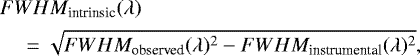
The measured and intrinsic widths of the different forbidden lines (full width at half maximum, FWHM) are presented in Table 3. The intrinsic FWHM is corrected for the instrumental broadening using the FWHM of the ThAr wavelength calibration lines using Eq. (1) and the obtained intrinsic FWHMs are transformed into velocity (km s−1) using Eq. (2), that is
 (1)
(1)
 (2)
(2)
where λn corresponds to the wavelength of forbidden emission line. More details on the determination of FWHMs are given in Decock et al. (2013). We assume the error on the FWHMinstrumental(λ) to be negligible. The FWHMs of different spectral emission lines that are measured on different nights were averaged and the dispersion of the measurements was used to estimate the error. No significant dependence on the nucleocentric distance was found, and therefore only measurements for the full slit are reported. The green [OI] 5577 line is wider than the [OI] red lines, which is similar to the observation made in water-dominated comets (Decock et al. 2015). A possible blend affecting [OI] 5577 Å has already been investigated and discarded by Decock et al. (2015). The observed [OI] red lines in C/2016 R2 are also wider compared to the values obtained in the majority of other comets (2.0 km s−1 vs. ~ 1.5 km s−1). Similar behavior is observed for the [CI] lines, with comparable values of the line widths. On the other hand, the faintness of the emission and imperfect subtraction of the scattered solar spectrum lead to significant errors while determining the [NI] line widths. Therefore, the difference between the derived widths of the two lines is not significant. Given the uncertainties, the widths of the [NI] lines are compatible with the widths of the [OI] and [CI] lines (see Table 3).
 |
Fig. 1 Partial Grotrian diagrams of atomic carbon (left), oxygen (centre), and nitrogen (right) showing various allowed and forbidden electronic transitions. The dashed lines represent the observed forbidden emission transitions in C/2016 R2. The values in parentheses represent the radiative lifetime of the excited state, which are taken from Wiese & Fuhr (2009) and Wiese et al. (1996). |
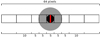 |
Fig. 2 Slit subdivision. The size of each subslit is indicated in pixels. The full slit extends over 64 pixels. The pixel size along the slit is 0.175′′ on average. Black and gray discs correspond to a seeing disc of 0.9′′ FWHM andthree times the seeing, respectively. The central pixel is denoted by a red rectangle. Adapted from Decock et al. (2015). |
Observed surface brightness of the various atomic forbidden emission lines in C/2016 R2 as a function of the nucleocentric projected distance.
Observed intensity ratios of atomic oxygen, carbon, and nitrogen emissions in C/2016 R2 at different nucleocentric projected distances.
Observed line widths of various forbidden atomic oxygen, carbon, and nitrogen emissions in C/2016 R2.
3 Model calculations
The model calculations of the atomic oxygen green- and red-doublet emission intensities are explained in detail in our earlier work (Bhardwaj & Raghuram 2012; Raghuram & Bhardwaj 2013, 2014; Decock et al. 2015; Raghuram et al. 2016). We have updated our model by including the atomic carbon and nitrogen emission lines. Here we present the model inputs considered for C/2016 R2 for the observational conditions of Opitom et al. (2019). We made the model calculations when the comet was at a distances of 2.8 au from the Sun and 2.44 au from the Earth. Since there is no information available on the radius of this comet, we assumed a typical value of 10 km for an Oort cloud comet.
3.1 Neutral distribution
The primary neutral composition of the cometary coma is taken as CO, CO2, H2O, N2, and O2. We have taken a CO gas production rate for this comet of 1.1 × 1029 s−1 (Biver et al. 2018). The relative abundances of CO2 and H2O with respect to CO are taken as 18 and 0.3%, respectively, from McKay et al. (2019). Based on the measured ionic emission intensity ratios, the relative volume mixing ratioof N2 is taken as 7% with respect to CO (Cochran & McKay 2018; Opitom et al. 2019; McKay et al. 2019). The recent Rosetta mass spectrometer in-situ measurements on 67P/Churyumov-Gerasimenko (Bieler et al. 2015; Altwegg et al. 2019) and subsequent investigation of data of the Giotto mass spectrometer from comet 1P/Halley (Rubin et al. 2015) suggest that O2 might be a common and abundant primary species in comets. In order to incorporate the photodissociation of O2 in the model, we assume an abundance of 1% with respect to CO. However, we vary this value to study its impact on the calculations of the [OI] G/R ratio. We adopted an outflow flow velocity of the neutral gas of 0.85 = 0.5 km s−1 at heliocentric distance rh (Cochran & Schleicher 1993; de León et al. 2019), and spherical symmetry is considered in the calculations.
The model calculates the neutral density profiles of the primary cometary species using the following Haser’s formula, which assumes spherical expansion of volatiles into the space with a constant radial expansion velocity (Haser 1957).
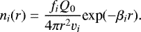 (3)
(3)
Here ni(r) is the number density of the ith neutral species at radial distance r, Q0 is the total gas production rate of the comet, and vi, fi, and βi represent the expansion velocity, fractional composition, and inverse of scale height of the ith neutral species. We consider N2 and CN to be the primary species producing N(2D) via dissociative excitation by both photons and photoelectrons. Assuming HCN is the parent source of CN, the neutral density profile of CN is calculated using Haser’s two-component formula (Haser 1957). For this calculation, we have taken HCN gas production as 4 × 1024 s−1 from the measurements of Biver et al. (2018). The role of other minor N-bearing species in producing N(2 D) is found to be negligible as discussed later.
Aforementioned cometary gas parameters, which resemble the observational conditions of C/2016 R2, are taken as baselineinputs for the model calculations. These baseline parameters are summarized in Table 4. However, we vary the neutral abundances used in the model to discuss the effect on the calculated emission ratios.
Summary of the baseline input parameters used in the model.
Production and loss reactions of N(2D), C(1 D), and C(1 S) incorporated into the chemical network of the coupled-chemistry emission model.
3.2 Atomic and molecular parameters
A detailed explanation of the input cross sections and chemical network used to calculate [OI] forbidden emission lines can be found in our earlier modeling work (Bhardwaj & Raghuram 2012). These model calculations account for various production and loss mechanisms of atomic oxygen in 1S and 1D states. We have added various production and loss reactions of metastable C(1 D), C(1 S) and N(2 D) in the [OI] chemical network to calculate the atomic carbon and nitrogen emission line intensities. Table 5 shows these additional set of reactions, which are incorporated into our new chemical network.
We have taken the electron impact cross section of N2 producing N(2 D) from Tabata et al. (2006). To incorporate production of N(2D) via photodissociation of N2, following the approach of Fox (1993), we assume an average photodissociation yield of 0.32. The impact of this assumption on the calculation of [CI]/[NI] emission ratio is discussed below. We have taken the photodissociation cross sections of CN producing C(1 D) and N(2 D) from El-Qadi & Stancil (2013). The photodissociation cross section of CO producing C(1 S) has never been reported in the literature. In order to incorporate this production path in the model, we assume that 0.5% of the total CO absorption cross section, above the dissociation threshold energy, leads to C(1 S) formation. However, we vary this value to fit the observed carbon emission intensity ratios, as discussed below. The collisional quenching rate coefficients of N(2D) by H2O, CO, CO2, and O2 are taken from Herron (1999), whereas, for C(1D) they are taken from Schofield (1979).
Calculated photodissociation frequencies (s−1) of major cometary species producing metastable states at 1 au.
 |
Fig. 3 Schematic presentation of the various chemical pathways of production and destruction of [CI], [OI], and [NI] metastable states in the cometary coma. Solid arrows, dashed arrows, and solid curved arrows represent the production channels of the excited species via photon and electron impact dissociative excitation of cometary neutrals, loss of excited species via radiative decay, and loss of excited species due to collisional quenching with neutrals, respectively. In the non-collisional region of the coma, all these photochemical reactions, except the collisional quenching reactions (curved arrows), determine the intensities of forbidden emission lines. |
3.3 Determination of emission intensity ratios
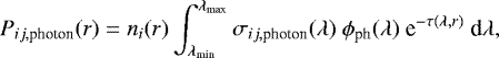
The solar radiation flux (ϕph(λ)) in the wavelength region 5–1900 Å is degraded in the cometary coma using the Beer-Lambert’s law. The photoelectron production rate spectrum is calculated as a function of electron energy at different radial distances. By incorporating the Analytical Yield Spectrum (AYS) approach, which accounts forthe degradation of electrons in the cometary coma based on the Monte Carlo technique, the suprathermal flux (ϕe (r, E)) is calculated as a function of electron energy (E) at the radial distance r. More detailsabout the calculation of suprathermal electron flux are given in Bhardwaj & Raghuram (2012).
Using the model degraded photon flux and steady state suprathermal electron flux profiles with the corresponding photon and electron impact excitation cross sections, we determined the volume production rate profiles for the different metastable state species in the coma using the following equations.
 (4)
(4)
 (5)
(5)
where Pij,photon(r) and Pij,electron(r) are the volume production rates of the jth metastable species due to the photon and electron impact dissociative excitation of the ith cometary neutral species, respectively, σij,photon and σij,electron are the respective photon and electron impact dissociative excitation cross sections of the ith neutral species producing the jth metastable state, λmin = 5 Å (Emin = 0 eV) and λmax = 1900 Å (Emax = 100 eV) are the respective lower and upper integration limits of the wavelength (energy) and τ(λ, r) is the optical depth of the medium for the photons of wavelength λ at the radial distance r. Table 6 shows the calculated photodissociation frequencies of the major cometary volatiles producing different metastable species at 1 au. The loss rate profiles of these excited states, which are mainly due to collisional quenching and radiative decay, are determined by incorporating the collisional chemistry in the coma. The major photochemical pathways producing the forbidden emission lines are schematically presented in Fig. 3.
The calculated production and loss rate profiles were used to obtain the number densities of metastable species (nj) by solving the following continuity equation:
 (6)
(6)
where r is the radial distance from the cometary nucleus, vj is the radial transport velocity, and Pj and Lj are the respective total production and loss rates of the jth metastable species. The transport velocities of the metastable species are taken from the measured intrinsic line widths (see Table 3). The calculated density profiles are converted into volume emission rates by multiplying the corresponding Einstein transition probabilities of the different emissions. The volume emission rate profiles are integrated along the line of sight to obtain surface brightness profiles. We also accounted for the optical seeing effect in determining the emission ratio as described in Decock et al. (2015). As explained above, seeing during the observations was 0.9″ for [OI] and [NI] emissions and 1.0″ for [CI] emissions.
We determined the [OI] G/R ratio and emission intensity ratios of C(1 D) to N(2D) – hereafter [CI]/[NI] ratio –, and carbon lines – hereafter [CI] ratio – using the following equations.
![\begin{align*} &[\textrm{OI}]\ \textrm{G/R}\ \textrm{ratio} = \frac{ I_{5577\ \text{\AA}}}{ I_{6300 \text{\AA}} + I_{6364 \text{\AA}}} = \frac{A_1\ [\textrm{O}(^1\textrm{S})]}{A_2\ [\textrm{O}(^1\textrm{D})]},\\ &[\textrm{CI}]/[\textrm{NI}]\ \textrm{ratio} = \frac{I_{9850 \text{\AA}} + I_{9824 \text{\AA}}}{I_{5200 \text{\AA}} + I_{5198 \text{\AA}}} = \frac{A_3\ [\textrm{C}(^1\textrm{D})]}{A_4\ [\textrm{N}(^2\textrm{D})]},\\ &[\textrm{CI}]\ \textrm{ratio} = \frac{I_{8727 \text{\AA}}}{I_{9850 \text{\AA}} + I_{9824 \text{\AA}}} = \frac{A_5\ [\textrm{C}(^1\textrm{S})]}{A_3\ [\textrm{C}(^1\textrm{D})],} \end{align*}](/articles/aa/full_html/2020/03/aa36713-19/aa36713-19-eq9.png)
where A1 (1.26 s−1), A2 (7.48 × 10⁻³ s−1), A3 (2.91 × 10⁻⁴ s−1), A4 (2.79 × 10⁻⁵ s−1), and A5 (0.6 s−1) are the total Einstein transition probabilities for the radiative decay of metastable states, which are taken from Wiese & Fuhr (2009), and [O(1 S)], [O(1 D)], [C(1 D)], [N(2 D)], and [C(1 S)] are the number densities.
We also studied the sensitivity of the model-calculated emission ratios to several parameters: the uncertainties associated with cross sections, neutral abundances, transport velocities of the species, and the collisional rate coefficients, as discussed in later sections.
4 Results
The calculated production rate profiles of atomic oxygen in 1 S (top panel) and 1D (bottom panel) states are presented in Fig. 4. This calculation shows that the formation of both O(1 S) and O(1 D) in the coma of C/2016 R2 occurs mainly due to the photodissociation of CO2. The photodissociation of CO contributes to about 20% of the total O(1S) production rate. The contribution of the photodissociative excitation of other oxygen-bearing species to the total O(1 D) production rate is small (<10%), within the observed projected distance, that is, 104 km. The electron impact dissociative excitation of oxygen-bearing species plays a minor role in producing these atomic oxygen metastable states.
The calculated loss frequency profiles of atomic oxygen in 1 S (top panel) and 1D (bottom panel) states are presented in Fig. 5. Radiative decay is the primary loss source of O(1 S) in the entire coma, as compared to collisional quenching. Whereas, the CO2 collisional quenching is the significant loss process for O(1D) for radial distances below 500 km. Above this radial distance, radiative decay is the prominent loss source.
The modeled C(1D) and N(2D) production rate profiles for different formation pathways are presented in Fig. 6. This calculation shows that the photodissociation of CO and N2 is the major formation processes of C(1D) and N(2D), respectively, whereas the contribution of the electron impact dissociative excitation to the total production rate is negligible. The role of CO2 photodissociation is minor (more than three orders of magnitude smaller than the CO photodissociation) in the total formation of C(1 D). Similarly, these calculations also show that the contribution from the dissociative excitation of CN in producing C(1 D) and N(2 D) is negligible to the total formation rate. Modeled loss frequency profiles of these excited states are presented in Fig. 7 and show that significant collisional quenching of C(1 D) and N(2 D) occurs via CO (>90% of the total) for radial distances below 3 × 10³ km. Above this radial distance, radiative decay is the major loss mechanism for both C(1 D) and N(2 D).
The modeled C(1S) production rate profile via photodissociation of CO and the loss profiles due to collisional quenching and radiative decay are presented in Fig. 8. Radiative decay of C(1 S) is found to be the dominant loss channel, which leads to [CI] 8727 Å emission, with an efficiency several orders of magnitude higher compared to the collisional quenching.
We calculated the timescale profiles for the loss of excited states due to both collisional quenching and radiative decay (chemical loss), which is reciprocal to the total loss frequency profiles as determined in Figs. 5, 7, and 8. The timescale for transport (advection) for the excited species is determined as tadv(r) ~r × [2vj (r)]−1, where vj is the mean radial velocity of the jth excited species as determined from the observations (see Table 3). These modeled timescale profiles for chemical loss and transport are plotted in Fig. 9. Here it can be seen that for radial distances larger than 100 km, the O(1 S) and C(1 S) chemical lifetimes are more than an order of magnitude smaller than the time required for transport. The timescales of O(1 D) due to chemical loss and transport are equal at the radial distance of 300 km, whereas this equality occurs at a radial distances of 100 and ~2 × 10³ km for C(1D). The N(2D) timescale for transport is smaller than the chemical lifetime in the entire coma.
After incorporating the previously mentioned production and loss mechanisms, we solved the 1D continuity equation (Eq. (6)) to calculate the radial density profiles of O(1 S), O(1 D), C(1 D), N(2 D), and C(1 S). These are plotted in Fig. 10. The peaks of O(1S) and C(1S) number densities occur close to the surface of the nucleus at radial distances below 20 km. The calculated N(2 D), C(1 D), and O(1D) density profiles have broad peaks at a radial distance of around 100 km, which is due to their long radiative lifetimes.
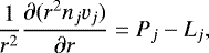
In the bottom panel of Fig. 11, we compare the modeled [OI] green-to red-doublet ratio with the observations. Using the baseline parameters as discussed in Sect. 3, we find that our modeled values are higher by a factor of three when compared to observations (hereafter Case-A). If we consider an O2 abundance of 30% with respect to the CO production rate (hereafter Case-B), instead of our assumed 1% in the baseline, our calculated [OI] G/R ratio is consistent with the observed emission ratio for radial distances below 1000 km. Above this radial distance the modeled ratio is about 40% higher than the observations. In this case, photodissociation of CO2 and O2 are the major sources of O(1S) and O(1 D), respectively. Due to the uncertainty in the CO2 photodissociative excitation cross section producing O(1D), as discussed in the following section, we increased the photodissociation rate by a factor of about three in our model calculations (hereafter Case-C). For this case, the modeled [OI] green-to-red-doublet emission ratio is in agreement with the observations.
Similarly, by using the baseline parameters as discussed in Sect. 3, the modeled [CI]/[NI] emission ratio profiles are found to be higher by a factor of three than the observations (hereafter Case-D, and see top panel of Fig. 11). In light of the uncertainty in the photodissociative excitation cross section, we decreased the photodissociation rate of CO producing C(1 D) by a factor of four (hereafter Case-E) in the model calculations. With these new dissociation rates, we find that the calculated emission ratios are in agreement with the observations. When we increase the N2 dissociative excitation rate producing N(2D) by a factor of about three (hereafter Case-F), we find that the modeled [CI]/[NI] emission ratio is consistent with the upper limit of the observations. The conditions for different case studies are summarized in Table 7.
If we assume that CO is the only parent source of the atomic carbon emissions, then the observed [CI] ratio should be equal to the ratio of the average branching fractions of CO producing C(1 S) and C(1 D). As described in the earlier section, we modeled the C(1S) density and calculated the 8727 Å emission intensity by assuming that 0.5% of the total CO absorption cross section leads to C(1 S) formation. Our modeled [CI] emission ratios for different yields along with the observation are plotted in Fig. 12 as a function of the nucleocentric projected distance. We find that the calculated [CI] ratio profiles are consistent with the observationswhen we vary the CO photodissociation yield between 1 and 1.5%.
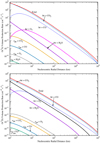 |
Fig. 4 Calculated O(1S) (top panel) and O(1D) (bottom panel) production rate profiles, for different photon and electron impact dissociative excitation reactions of major cometary volatiles in C/2016 R2 when it was at 2.8 au from the Sun. The total gas production rate of CO is taken as 1.1 × 1029 s−1 with 0.3% H2O, 18% CO2, and 1% O2 with respect to carbon monoxide. Here, hν represents a solar photon and eph is a suprathermal electron. |
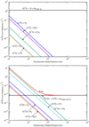 |
Fig. 5 Modeled O(1S) (top panel) and O(1D) (bottom panel) loss frequency profiles via collisional quenching of the major cometary volatiles and radiative decay in C/2016 R2. The input conditions are the same as in Fig. 4. |
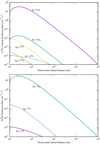 |
Fig. 6 Calculated C(1D) (top panel) and N(2D) (bottom panel) production rate profiles, for different photon and electron impact dissociative excitation reactions of the major cometary volatiles, in C/2016 R2. Photodissociation and electron impact dissociation of CN producing N(2 D) production rate profiles are plotted after multiplying them by a factor of ten. The input conditions are the same as explained in Fig. 4. Here, hν represents a solar photon and eph is a suprathermal electron. |
 |
Fig. 7 Calculated C(1D) (top panel) and N(2D) (bottom panel) loss frequency profiles via collisional quenching of major cometary volatiles and radiative decay in C/2016 R2. The input conditions are the same as in Fig. 4. |
 |
Fig. 8 Calculated production rate (left y-axis) and loss frequency (right y-axis) profiles of C(1 S) in C/2016 R2. The collisional quenching rates are plotted after multiplying them by a factor of 103. The input conditions are the same as in Fig. 4. |
 |
Fig. 9 Calculated chemical lifetime profiles of N(2D), C(1 D), O(1 D), C(1 S), and O(1S) due toboth collisional quenching and radiative decay in C/2016 R2. For comparison, the timescale for transport of metastable species (red line) is calculated for 2 km s−1 radial velocity. The input conditions are the same as in Fig. 4. |
 |
Fig. 10 Calculated number density profiles of O(1S), O(1 D), C(1 D), N(1 D), and C(1 S), by incorporating various photon and electron impact dissociative excitation reactions of the major cometary volatiles in C/2016 R2. The input conditions are the same as in Fig. 4. |
5 Discussion
The photochemical processes such as dissociative excitation of cometary coma species, collisional chemistry, and radial transport of metastable species determine the observed emission intensity ratios. When we use our baseline input parameters, as explained in Sect. 3, the calculated [OI] G/R and [CI]/[NI] ratios are higher by a factor of about three compared to the observations. In order to study the discrepancies between the modeled and the observed emission ratios, we examined the effects of uncertainties associated with the input parameters, which are discussed below.
Summary of the different case studies for calculating the [OI] G/R and the [CI]/[NI] emission ratios.
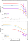 |
Fig. 11 Comparison between modeled and observed [CI] to [NI] (top panel) and [OI] G/R (bottom panel) emission ratios in C/2016 R2. The calculated emission ratios for the input conditions are explained in Fig. 4. The calculated emission ratios for Case-A and Case-D are plotted after multiplication by a factor of 0.3. See the main text and Table 7 for more details about the conditions of Case-A to Case-F. |
5.1 Effect of the neutral species abundances
In a water-dominated coma, H2O photodissociation is the major source of O(1D). But the observations of Biver et al. (2018) showed that H2O abundance with respect to CO cannot be more than 10%. The recent McKay et al. (2019) observations suggest much lower water abundance (0.3% with respect to CO), which is also observed by Opitom et al. (2019). Even by assuming an H2O abundance of 10% relative to CO, we find that H2O is playing no role in determining the [OI] G/R ratio. This calculation suggests that CO2 mainly governs both the green and red-doublet atomic oxygen emission intensities and the contribution from other excitation processes is negligible. The derivation of water production rates based on the observed oxygen emission lines would of course lead to an overestimation of H2O abundance in this comet.
Biver et al. (2018) observed several other O-bearing species such as CH3OH, H2CO, HNCO, NH2CHO, CH3CHO, HCOOH, SO, and SO2 in this comet. The branching ratios as determined by Huebner et al. (1992) suggest that these species do not have direct production channels for O(1S) and O(1D). Moreover, these species are observed with very low abundance, namely more than two orders of magnitude lower than CO (Biver et al. 2018). Therefore, the contribution of these species to the production of [OI] emission lines can be neglected.
The modeling work of Cessateur et al. (2016a) has suggested that O2 can play a significant role in determining the [OI] G/R ratio. By incorporating a small O2 abundance of 1% of the CO production rate we find that the contribution of O2 dissociative excitation is very small (more than two orders of magnitude to the total) in producing O(1 S) whereas it is the third most important source of O(1D) for radial distances above 30 km (see Fig. 4). By increasing the O2 abundance to 4% of CO, we find that about 30% of O(1D) is produced from the photodissociation of O2 and 50% of the total is coming from CO2. In this case, O(1S) is mainly (> 80%) produced from the photodissociation of CO2 and the role of O2 is small (< 1%). This calculation suggests that O2 is a potential source of O(1D), after CO2, when its abundance is substantial (>5%).
The in-situ measurements of the Rosetta mass spectrometer have shown that O2 is present in the coma of comet 67P with a mean abundance of about 2% (Altwegg et al. 2019). During the Rosetta mission, Bieler et al. (2015) showed that the O2 relative abundance with respect to H2O can be as high as 15%. It should be noted that the mass spectrometer abundances are based on the observations made at the spacecraft position. However, the Alice UV spectrometer onboard Rosetta can observe the spatial distribution of neutrals in the entire cometary coma based on the emission intensities (Feldman et al. 2018). From Alice limb view observations, Keeney et al. (2017) found that the O2 /H2O relative abundance ratio in 67P coma varies between 11 and 68%, with a mean value of 25%. These observations suggest that O2 could be present in large amounts in cometary comae. We also increased the O2 relative abundance to 30% of CO to verify its impact on the [OI] G/R abundance ratio. By considering such a large O2 abundances, we show that the model calculated [OI] G/R ratio is close to the observation (see bottom panel of Fig. 11) for radial distances below 103 km. However, the calculated emission ratios are higher by about 40% compared to the observation in the noncollisional zone, that is, for radial distances greater than103 km (also seeFig. 5). This calculation suggests that this comet could possibly contain a significant amount of molecular oxygen (about 30% relative to CO).
Similarly, we studied the discrepancy between the modeled and observed [CI]/[NI] emission ratio by varying the neutral abundances. We considered CO2 and CO as the primary molecules producing C(1D) and CN, and N2 to be the primary source of N(2D). The role of CO2 in producing C(1D) is negligible compared to that of CO. This is mainly due to the significant difference between the photodissociative excitation cross sections of CO and CO2 producing atomic carbon (about two orders of magnitude; see Huebner et al. 1992). C(1 D) can be produced directly from the dissociation of CO whereas it is a two-step process for CO2. By increasing the CO2 abundance equal to that of CO, we find that CO is still the dominant source of C(1 D), which suggests that [CI] emission lines are governed only by the CO photodissociation and the role of CO2 in producing carbon emission lines can be neglected.
In order to match the observed [CI]/[NI] emission ratio, the N2 /CO volume mixing ratio should be altered by a factor of three either by decreasing the CO or by increasing the N2 production rates. Since the comet is moving towards the Sun, we do not expect a decrease in the CO sublimation rate during the observation period. However, large N2 abundances (>10%) are not expected either, unless there is a cometary outburst during the period of observation. Moreover, different observations have confirmed that the N2 abundance in this comet is about 7% relative to CO (Cochran & McKay 2018; Biver et al. 2018; Opitom et al. 2019). We therefore do not expect this comet to have a large enough N2 abundance (>10%) to produce the observed [CI]/[NI] emission ratio. We also investigated other N-bearing species capable of producing N(2 D) in significant amounts. Singh et al. (1991) proposed that the formation of metastable nitrogen atoms in 2 D state is possible thanks to the photodissociation of CN, but our modeled production rate profiles of N(2 D) show that the contribution from CN is negligible compared to the photodissociation of N2 (see Fig. 6). Moreover, Opitom et al. (2019) estimated the CN production rate as 3 × 1024 s−1, which is five orders of magnitude smaller than the CO gas production rate and cannot be the dominant source of [CI] and [NI] emission lines. Similarly, the observations of various N-bearing species, such as HCN, CH3CN, HC3N, HNCO, and NH2CHO by Biver et al. (2018) and McKay et al. (2019) show that their relative abundances in the coma are very small (<1%) compared to N2, while the Huebner et al. (1992) compilation of photodissociation cross sections does not suggest direct dissociative excitation channels to produce N(2 D). We therefore conclude that the atomic nitrogen emission is only governed by the photodissociation of N2 in C/2016 R2.
The Opitom et al. (2019) observations clearly show that C2 and C3 molecules are only present in negligible amounts in this comet. Unlike the major volatiles, C2 and C3 are not directly produced in the coma via sublimation of ices in the nucleus. The formation and destruction of these species form part of a complex chemistry. By considering the long-chain carbon-bearing species in the coma, Hölscher (2015) studied the density distribution of C2 and C3 in the comae of different comets. Based on these calculations, we estimated that the production rate of C(1 D) via dissociation of C2 and C3 is smaller than the photodissociation rate of CO by more than three orders of magnitudes. However, the calculation of C2 and C3 number density profiles using the complex chemical network as described by Hölscher (2015) is beyond the scope of the present work.
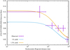 |
Fig. 12 Comparison between modeled and observed [CI] 8727 Å/ (9850 Å + 9824 Å) emission intensity ratio profiles in C/2016 R2. Solid curves represent the modeled emission ratios for two different photodissociation yields of C(1 S). |
5.2 Effect of the cross sections
The uncertainty in the photodissociation cross section of CO2 producing O(1 D) could be the reason for the difference between the modeled and observed [OI] G/R ratios. Lawrence (1972) experimentally determined the photodissociation yield of CO2 producing O(1S) as high as 1 in the wavelength range 1000–1150 Å. We considered this measured yield to calculate the CO2 dissociation rate to produce O(1S). The cross section for O(1D) formation via CO2 dissociative excitation is not reported in the literature, as noticed by Huestis & Slanger (2006). Huebner et al. (1992) constructed these photodissociation cross sections of CO2 assuming a dissociation branching ratio close to 1 in the wavelength region 1000–1665 Å. This assumption contradicts the Lawrence (1972) experimentally determined branching ratio. Both O(1 D) and O(1 S) cannot be produced with 100% yield in the same wavelength region. Slanger et al. (1977) also measured the quantum yield of O(1 S) for photodissociation of CO2 and found a sudden dip in the yield around 1089 Å. Therefore, there is an uncertainty associated with the Huebner et al. (1992) recommended cross sections which can impact our calculated [OI] G/R emission ratio. There have been several recent experimental developments in detecting O(1 D) via the photodissociation of CO2 (Sutradhar et al. 2017; Lu et al. 2015; Song et al. 2014; Schmidt et al. 2013; Gao & Ng 2019; Pan et al. 2011). But these measurements are limited to a small energy range (<1 eV) and do not provide the O(1D) yield over a wide wavelength range (from dissociation threshold to 1000 Å) which is essential to determine the average dissociation ratio of O(1 S)/O(1D) in the photodissociation of CO2.
As discussed in the earlier section, the photodissociation of CO2 is the major source of O(1S) in the coma. This is mainly due to the larger photodissociation rate of CO2 than CO and H2O (a factor around 20 higher compared to other O-bearing species; see Table 6, Fig. 4, and Huebner et al. 1992). Similarly, CO2 can also produce O(1D) by a factor of 3 more efficiently than any other O-bearing species. Hence, if CO2 is the majorproduction source of oxygen lines, then the observed [OI] G/R ratio in the non-collisional region (i.e., above 103 km, see Fig. 5) should match the ratio of CO2 dissociation rates producing O(1S) and O(1D).
Our calculations suggest that the photodissociation of CO is the second-most important source of [OI] emission lines (see Fig. 4). Since most of the O(1S) and O(1D) are produced from CO2, the uncertainties associated with the CO dissociation cross sections cannot play a significant role in determiningthe [OI] G/R ratio. Moreover, the respective dissociation threshold energies of CO producing O(1 D) and O(1 S) states are 14.35 and 16.58 eV, which are more than the ionization threshold, that is, 14 eV. Due to the proximity of the threshold energies, most of the UV radiation absorbed by CO turns into ions rather than producing O(1 S) and O(1 D). Therefore, CO is not an efficient source of [OI] emission lines to determine the [OI] G/R ratio compared to CO2.
In our earlier work, we theoretically determined [OI] G/R ratios of 0.04, 0.6, 1, and 0.04 for the photodissociation of H2O, CO2, CO, and O2, respectively (Bhardwaj & Raghuram 2012; Raghuram & Bhardwaj 2013; Raghuram et al. 2016). If CO2 is the only source of these emission lines, by using the photodissociation cross sections from the baseline model (also see Bhardwaj & Raghuram 2012), our model suggests that the [OI] G/R ratio should be around 0.6 for the noncollisional region. However, the observed ratio in this comet is only about 0.2 between radial distances of 2 × 10³ and 1 × 10⁴ km, where the radiative decay is the only loss process (see Fig. 11). We show in the following section that the collisional quenching can alter the observed [OI] G/R ratio only for radial distances less than 2 × 10³ km (see Fig. 5). Because CO2 is the major source of [OI] emissions and there is a large uncertainty associated with the CO2 photodissociative cross section in producing O(1D), we increased the photodissociation rate by a factor of three (see Case-C in Fig. 11). For this value of the photodissociation rate, the observed and modeled [OI] G/R ratios are consistent. Hence, based on the comparison between the modeled and observed [OI] G/R ratio profiles, we suggest to increase the Huebner et al. (1992) recommended photodissociation cross section of CO2 producing O(1 D) by a factor of three.
In our modeling calculations on different comets at different heliocentric distances, we show that H2O is the major source of O(1D) (Bhardwaj & Raghuram 2012; Raghuram & Bhardwaj 2013, 2014; Decock et al. 2015; Raghuram et al. 2016). Even though the photodissociation rate of H2O producing O(1 D) is comparable (a factor of 1.5 higher) to that of CO2 (see, Huebner et al. 1992), CO2 became the prominent source of green- and red-doublet emission lines due to the very low water abundance in this comet. Therefore, this new value of CO2 dissociation rate producing O(1D) does not contradict the conclusions of our earlier calculations done in the water-dominated cometary comae.
Similarly, the discrepancy between the modeled and observed [CI]/[NI] emission ratios could also be due to the uncertainties in the photodissociation cross sections of CO and N2. Shi et al. (2018) recently determined the branching ratio for CO producing C(1 D) in the wavelength range 905–925 Å. These latter authors found that the pre-dissociation of CO leads to about 20% formation of C(1 D) and the rest into carbon and oxygen ground and 1D states, respectively. Huebner et al. (1992) do not account for pre-dissociation channels in the formation of C(1 D). The cross section is constructed based on the assumptions of McElroy & McConnell (1971). By decreasing the CO photodissociation rate by a factor of four, we find that the modeled [CI]/[NI] emission ratio is consistent with the observation (see Case-E in Fig. 11). This calculation shows that the uncertainty associated with the Huebner et al. (1992) CO photodissociation cross section could be a reason for the discrepancy between the modeled and the observed ratios. We therefore suggest that the photodissociation cross section of CO producing C(1 D) should be revised based on the recently determined branching ratios.
We have taken a mean average branching ratio of N(2 D) of 0.32 following the approach of Fox (1993) calculations on Mars and Venus atmospheres. Song et al. (2016) measured branching ratios for the photodissociation of N2 producing N(2D) in the wavelength region 816.3–963.9 Å as high as 1. By increasing the N2 photodissociation rate by a factor of three, we find that the modeled [CI]/[NI] emission ratio is consistent with the upper limit of the observations (see Case-F in Fig. 11). These calculations suggest that the uncertainties associated with the photodissociation cross sections of CO and N2 are the main reason for the discrepancy between the modeled and the observed [CI]/[NI] emission ratios.
Besides the cross sections of neutral species, the modeled photodissociation frequencies also depend on the solar activity. Considering the solar activity, Huebner et al. (1992) showed that the calculated photodissociation frequencies of neutrals can vary by a factor of about two from solar minimum to maximum. Since the observations of C/2016 R2 were all made in February 2018, which is during a minimum range of time and solar minimum condition, we do not expect the solar activity to significantly influence the modeled dissociation frequencies and subsequently the calculated emission ratios.
5.3 Effect of collisional quenching rates
The collisional quenching of atomic oxygen can alter the observed emission ratio for radial distances smaller than 2 × 10³ km (see Fig. 9). Owing to a short radiative lifetime (0.75 s, Wiese & Fuhr 2009), the collisional quenching of O(1 S) is not significant in the entire coma. But for O(1D), the quenching is an important loss process up to radial distances of 2 × 10³ km (see Fig. 5). By assuming a collisional quenching source of O(1 D), which is an order of magnitude higher than that of CO2, we are able to alter the G/R ratio by a factor of 2, but only up to radial distances of ≃103 km. Therefore, the observed [OI] G/R ratio, beyond 103 km radial distances, is purely a function of dissociative excitation of CO2.
The collisional quenching is significant for both C(1 D) and N(2 D) due to theirradiative lifetimes of about 3500 s and 10 h, respectively, up to radial distances of 2 × 10³ km (see Fig. 7). However, we could not find a significant change in the calculated [CI]/[NI] emission ratios by varying the quenching rates. Our calculated lifetime profiles of these excited species show that the transport of N(2 D) is a more important loss process than the collisional quenching in the coma (see Fig. 9). In this figure, the C(1 D) collisional quenching can be seen to affect the modeled [CI]/[NI] emission ratio only for radial distances below 50 km. By assuming an unknown collisional reaction in the coma with a quenching rate an order of magnitude higher than that of CO, we find the modeled [CI]/[NI] emission ratio is not changing for radial distances beyond 4 × 10³ km.
The collisional quenching is a strong barrier inhibition in measuring the photodissociation cross section of species producing metastable states. Because of the long lifetimes and also the excess velocities acquired during dissociation, most of the metastable species drift away from the spectrometer field of view and also collide with the walls of the chamber which makes it very difficult to measure such cross sections in the laboratory (Kanik et al. 2003). Owing to natural vacuum conditions, the metastable species produced via cometary species can survive for longer and are transported to large radial distances from the origin of production before they de-excite to ground state via radiative decay. Therefore, in the absence of collisions, the observed cometary forbidden emissions lines can be used to study the dissociation properties of the respective parent species which makes comets unique natural laboratories.
5.4 Effect of transport
When the mean lifetime of a species is more controlled by collisions or radiative decay than radial transport, we can consider that the species is under photochemical equilibrium (PCE). The calculated lifetime profiles presented in Fig. 9 show that O(1 S) and C(1 S) are in PCE in the entire cometary coma. The transport of C(1D) and O(1D) is important for radial distances above 50 and 100 km, respectively. Due to the large radiative lifetime of N(2 D) – about 10 h –, transport plays a significant role in determining its number density in the coma. These calculations suggest that the role of transport in determining the [OI] G/R ratio is insignificant whereas it is important for the [CI]/[NI] emission ratio.
Huebner et al. (1992) determined the mean excess energies released in the photodissociation of N2 and CO as 3.38 and 2.29 eV, respectively. Using these calculated excess energies, we estimated the mean ejection velocities of N(2 D) and C(1 D) as 4.77 and 4.59 km s−1, respectively, (cf. Wu & Chen 1993). Using these theoretically estimated mean velocities in the model, we found our modeled [CI]/[NI] emission ratio is higher by a factor of two. If we assume that our estimated mean excess velocities of C(1 D) and N(2 D) are realistic, then a factor of two in CO photodissociation rate will be sufficient to explain the observed [CI]/[NI] ratio. However, our observed line widths suggest that C(1D) and N(2D) did not acquire velocities as calculated by Huebner et al. (1992).
Our theoretically estimated N(2D) and C(1D) excess velocities are based on the calculation of Huebner et al. (1992). These values are higher than our mean velocities derived from the observations by about a factor of two (see Table 3). However, it should be noted that Huebner et al. (1992) used a reference solar flux for solar minimum condition to determine the excess energy released in the photodissociation. The solar flux as observed by the comet determines the mean excess energy released in the photodissociation and subsequently the widths of the spectral lines. The determination of excess energies released in the photochemical process requires the knowledge of the solar radiation flux interacting with the coma and also the absolute branching fractions over a wide wavelength range, which are the strong constraints to compute the mean excess velocities.
The role of transport on O(1D) and O(1S) is not significant in determining the [OI] G/R ratio. This can be understood from the calculations of the timescales for chemicallifetime and transport presented in Fig. 9. We calculated density profiles of all the metastable species using the derived excess velocities from the observed line widths. The Huebner et al. (1992) theoretical calculations at 1 au suggest that excess energies of about 4 eV will be released in the photodissociation of CO2 producing O(1 D). Around 65% of excess energy released in the dissociation would produce atomic oxygen with an excess velocity of about 5 km s−1. By increasing the radial velocity of the metastable species to about 5 km s−1, our calculated [OI] G/R ratio is higher by a factor of five compared to the observations. The role of transport in determining the O(1 S) density is negligible due to its small lifetime of about 1 s, whereas it can affect O(1 D) up to radial distances of 104 km. Due to the lack of measured cross sections of O(1D) via CO2 it is difficult to determine the excess energy released in the photodissociation.
5.5 Line widths
The observed FWHMs of the emission lines mainly depend on the mean kinetic energy of the excited species which are produced in the dissociative excitation. Our calculations suggest that the influence of collisional quenching on the line width is up to radial distances of 103 km (see Figs. 5 and 6). In the observed spectra, we find that the measured line widths of the observed emissions do not vary significantly as a function of the nucleocentric distance. Moreover, the radiative efficiency of all the metastable states, except for O(1 S), is close to unity for radial distances above 103 km, where most of the emission intensity occurs. Since the emission intensity in the observed spectra is mostly determined by the radiative decay of the excited species, we can neglect the contribution of collisional broadening while converting the line width to the mean velocity of the excited species.
The line widths reported in Table 3 show that the atomic oxygen green line is broader than the red-doublet lines, and this is also consistent with the observation made in other comets (Cochran 2008; Decock et al. 2013, 2015). This can be explained by the excess velocity of oxygen atoms acquired during the CO2 photodissociation. The formation of O(1S) via CO2 dissociative excitation occurs at shorter wavelengths compared to that of O(1 D), which leads to more excess energy release and results in higher mean velocity. Raghuram & Bhardwaj (2013) calculated the mean excess energy profiles of O(1S) and O(1D) in comet Hale–Bopp and showed that the photodissociative excitation reactions produce O(1 S) with greater excess energies than those of O(1D). Based on the measured line widths, Cochran (2008) suggested that the wider green line could be due to the involvement of different energetic photons in dissociating a single parent species and/or dissociation of multiple species, producing O(1 S) and O(1 D) with different excess energies. Our model calculations suggest that CO2 mainly produces both green- and red-doublet emission lines and the involvement of other species is small (see Fig. 4). We therefore argue that the observed green line is wider than the red-doublet mainly because CO2 is dissociated by high energetic solar photons which produce O(1S) with large excess velocities.
Similarly, the [CI] 8727 Å line is wider than the 9850 Å line and this could also be due to the involvement of high energetic photons in the photodissociation of CO. The dissociation thresholds of CO producing C(1 D) and C(1 S) are 12 and 14 eV, respectively. Therefore, the CO dissociation by highly energetic photons leads to more excess velocity for C(1 S) than for C(1 D). Moreover, the production rate of atomic carbon via CO2 dissociative excitation is very low compared to that of CO (Huebner et al. 1992). Therefore, the role of CO2 in the C(1 S) formation can be neglected. As shown in Fig. 1, the radiative decay of C(1 P) can also populate C(1D), which additionally contributes to the emission intensities at wavelengths of 9824 and 9850 Å. Because this formation channel occurs at energies higher than 18 eV, where most of the CO turns into ion, the contribution from radiative decay of C(1 P) can be neglected in the formation of C(1S).
The line widths of our observed red-doublet emissions are similar, which suggests that the O(1 D) is released with a mean excess velocity of 2.01 km s−1 from dissociative excitation (see Table 3). The derived line widths for the 5198 and 5200 Å emissions, which arise due to radiative decay of the same excited state, that is, N(2 D) – see Fig. 1 –, are compatible with the uncertainties in the observation.
5.6 The doublet emission ratios
The radiative decay of metastable states such as C(1D), O(1 D), and N(2D) to the ground state produces doublet emissions due to splitting in the sub-levels of the electronic states (see Fig. 1). The observed intensity ratio of these doublet emission lines should therefore be equal to the ratio of the Einstein decay probability coefficients of the corresponding transitions. The [CI] 9824 Å emission line is strongly contaminated by telluric absorption line which prevented us from determining the precise [CI] 9824/9850 emission ratio. On the contrary, the measured [OI] ratio over the full slit is well determined and is in agreement with the theoretical value (Wiese et al. 1996). Based on the theoretical calculations of Tachiev & Froese Fischer (2002), Wiese & Fuhr (2007) recommend a transition probability ratio of the [NI] doublet equal to 2.6. Our observations show that this value is 1.22 ± 0.09, which is nearly half the Wiese & Fuhr (2007) value. Sharpee et al. (2005) noticed that there is a significant difference between the calculated and observed [NI] emission ratios. These latter authors measured the [NI] emission ratio in the night glow of the terrestrial spectrum and found it to have an average value of 1.76. In the terrestrial atmosphere, strong collisions between N(2 D) and other species can alter the statistical population of atomic nitrogen excited levels, which subsequently affects the intensity ratio of the [NI] emission lines. The Hernandez & Turtle (1969) and Sivjee et al. (1981) measurements show that the [NI] ratio varies between 1.2 and 1.9. Sivjee et al. (1981) calculated an emission ratio profile by considering major collisional quenching reactions of N(2D). These latter authors found that the [NI] ratio can be as low as 1.1. Our calculated lifetime profiles show that throughout the coma, the N(2 D) density is essentially determined by transport rather than quenching due to the poor collisional interactions with other cometary species (see Fig. 9). Therefore, the role of collisional quenching in the observed [NI] ratio can be neglected. Based on the observations and modeling, we argue that the measured [NI] emission ratio is mainly due to the intrinsic transition probability ratio of sub-levels of N(2 D). As discussed in the earlier section, it is difficult to measure the [NI] ratio experimentally due to the long lifetime of N(2 D), namely ~10 h, while the collisional quenching in the terrestrial environment can alter the observed [NI] ratio significantly. The cometary spectroscopic observationsare therefore a new natural way to explore atomic and molecular properties that cannot be determined in the laboratory.
6 Summary and conclusions
Recent observations of C/2016 R2 show that its coma has a peculiar composition compared to most comets observed so far. Several forbidden emission lines were detected in the optical, some for the first time, using UVES mounted on the Very Large Telescope (Opitom et al. 2019). The observed atomic carbon, oxygen, and nitrogen forbidden emission transitions are modeled under the frame-work of a coupled-chemistry emission model, by incorporating the major production, loss, and transport mechanisms of C(1 D and 1 S), O(1 D and 1 S), and N(2 D) species. The observation of these forbidden emissions in a water-depleted comet is a novel and unique case to study the photochemistry of the metastable states and their emission processes in such a cometary coma. The major conclusions drawn from both observations and modeling are as follows.
- 1.
The major source of [OI], [CI], and [NI] emissions is found to be the photodissociation of CO2, CO, and N2, respectively.
- 2.
The collisional quenching of all the metastable states, except for O(1S) and C(1S), is significant for radial distances below 3 × 10³ km. The collisional quenching of C(1D) and N(2D) occurs mainly by CO whereas it is by CO2 for O(1D).
- 3.
In this water-depleted coma, the observed [OI] G/R emission ratio is found to vary between 0.3 and 0.18, which is smaller than the Festou & Feldman (1981) value of 0.9 for a CO2 coma by a factor of three or more. This lower value indicates that the observed [OI] G/R emission ratio is not a parameter that can be used to identify the major parent source of [OI] emissions in the cometary coma.
- 4.
The observed width of the green emission line is larger mainly because of the photodissociation of CO2 that occurs by high energetic photons, which results in O(1S) having a large excess mean velocity. Since the photodissociation of CO2 is the only source of the oxygen emission lines, the involvement of multiple species in producing the larger green line width can be discarded in this comet.
- 5.
By comparing the observed and modeled [CI]/[NI] emission ratios in this comet, we suggest that the photodissociation cross section of CO producing C(1D) should be reduced by a factor of four.
- 6.
Using a high molecular oxygen abundance (about 30% with respect to CO), our modeled [OI] G/R ratio is consistent with the observations for radial distances below 103 km. Above this radial distance, the modeled values are higher by 40% than the observations. This suggests that the photodissociation of molecular oxygen is a possible source of these emissions lines.
- 7.
Based on the observations and modeling of these emissions we suggest that in a water-depleted and CO- and CO2-rich cometary coma, which could be the case for comets observed at large (>3 au) heliocentric distances as H2O is not yet sublimating, the observed [OI] emissions are mainly governed by CO2.
- 8.
The modeling of the [OI] G/R ratio suggests that the ratio of dissociation frequencies of CO2 producing O(1S) to O(1D) should be around 0.2. Similarly, the modeled [CI]/[NI] emission ratio suggests that the mean branching fraction of CO for the production of C(1D) should be smaller than the Huebner et al. (1992) values by a factor of between three and five. The observed emission ratios of metastable species in the noncollisional region is a new way to constrain the mean branching ratio of metastable species produced via photodissociative excitation.
- 9.
In spite of having a long radiative lifetime (~10 h), N(2D) is mainly controlled by transport rather than collisional quenching. Therefore, the observed [NI] ratio of 1.22, which is smaller than the terrestrial measurement by a factor of 1.4, is mainly due to the intrinsic transition probability ratio.
- 10.
The simultaneous observation of both [CI] 8727 Å and 9850 Å emission lines allowed us to constrain the yield of CO photodissociation producing C(1S). This is about 1% of the total absorption cross section, which had not previously been determined in the laboratory. This suggests that cometary spectroscopic observations serve as a natural tool to explore their atomic and molecular properties.
Acknowledgements
S.R. is supported by Department of Science and Technology (DST) with Innovation in Science Pursuit for Inspired Research (INSPIRE) faculty award [Grant: DST/INSPIRE/04/2016/002687], and he would like to thank Physical Research Laboratory for facilitating conducive research environment. D.H. and E.J. are FNRS Senior Research Associates. The authors would like to thank the anonymous reviewer for the valuable comments and suggestions that improved the manuscript.
References
- Altwegg, K., Balsiger, H., & Fuselier, S. A. 2019, ARA&A, 57, 113 [NASA ADS] [CrossRef] [Google Scholar]
- Bhardwaj, A. 1999, J. Geophys. Res., 104, 1929 [NASA ADS] [CrossRef] [Google Scholar]
- Bhardwaj, A., & Haider, S. A. 2002, Adv. Space Res., 29, 745 [NASA ADS] [CrossRef] [Google Scholar]
- Bhardwaj, A., & Raghuram, S. 2012, ApJ, 748, 13 [NASA ADS] [CrossRef] [Google Scholar]
- Bieler, A., Altwegg, K., Balsiger, H., et al. 2015, Nature, 526, 678 [Google Scholar]
- Biver, N., Bockelée-Morvan, D., Paubert, G., et al. 2018, A&A, 619, A127 [NASA ADS] [CrossRef] [EDP Sciences] [Google Scholar]
- Cessateur, G., de Keyser, J., Maggiolo, R., et al. 2016a, J. Geophys. Res. Space Phys., 121, 804 [NASA ADS] [CrossRef] [Google Scholar]
- Cessateur, G., De Keyser, J., Maggiolo, R., et al. 2016b, MNRAS, 462, S116 [CrossRef] [Google Scholar]
- Cochran, A. L. 2008, Icarus, 198, 181 [NASA ADS] [CrossRef] [Google Scholar]
- Cochran, A. L., & McKay, A. J. 2018, ApJ, 854, L10 [NASA ADS] [CrossRef] [Google Scholar]
- Cochran, A. L., & Schleicher, D. G. 1993, Icarus, 105, 235 [Google Scholar]
- de León, J., Licandro, J., Serra-Ricart, M., et al. 2019, Res. Notes Am. Astron. Soc., 3, 131 [Google Scholar]
- de Val-Borro, M., Milam, S. N., Cordiner, M. A., et al. 2018, ATel, 11254 [Google Scholar]
- Decock, A., Jehin, E., Hutsemékers, D., & Manfroid, J. 2013, A&A, 555, A34 [NASA ADS] [CrossRef] [EDP Sciences] [Google Scholar]
- Decock, A., Jehin, E., Rousselot, P., et al. 2015, A&A, 573, A1 [NASA ADS] [CrossRef] [EDP Sciences] [Google Scholar]
- Delsemme, A. H., & Combi, M. R. 1976, ApJ, 209, L149 [NASA ADS] [CrossRef] [Google Scholar]
- Delsemme, A. H., & Combi, M. R. 1979, ApJ, 228, 330 [NASA ADS] [CrossRef] [Google Scholar]
- El-Qadi, W. H., & Stancil, P. C. 2013, ApJ, 779, 97 [NASA ADS] [CrossRef] [Google Scholar]
- Feldman, P. D. & Brune, W. H. 1976, ApJ, 209, L45 [NASA ADS] [CrossRef] [Google Scholar]
- Feldman, P. D., Weaver, H. A., Festou, M., et al. 1980, Nature, 286, 132 [NASA ADS] [CrossRef] [Google Scholar]
- Feldman, P. D., Festou, M. C., Tozzi, P., & Weaver, H. A. 1997, ApJ, 475, 829 [NASA ADS] [CrossRef] [Google Scholar]
- Feldman, P. D., Cochran, A. L., & Combi, M. R. 2004, Comets II, Spectroscopic investigations of fragment species in the coma, eds. M. C. Festou, H. A. Weaver, & H. U. Keller (Tucson: University of Arizona Press), 425 [Google Scholar]
- Feldman, P. D., A’Hearn, M. F., Bertaux, J.-L., et al. 2018, AJ, 155, 9 [NASA ADS] [CrossRef] [Google Scholar]
- Festou, M. C.,& Feldman, P. D. 1981, A&A, 103, 154 [NASA ADS] [Google Scholar]
- Fink, U., & Johnson, J. R. 1984, AJ, 89, 1565 [NASA ADS] [CrossRef] [Google Scholar]
- Fox, J. L. 1993, J. Geophys. Res., 98, 3297 [NASA ADS] [CrossRef] [Google Scholar]
- Furusho, R., Kawakitab, H., Fusec, T., & Watanabe, J. 2006, Adv. Space Res., 9, 1983 [NASA ADS] [CrossRef] [Google Scholar]
- Gao, H., & Ng, C.-Y. 2019, Chin. J. Chem. Phys., 32, 23 [CrossRef] [Google Scholar]
- Haser, L. 1957, Bull. Acad. Roy. Sci. Liege, 43, 740 [NASA ADS] [Google Scholar]
- Hernandez, G., & Turtle, J. P. 1969, Planet. Space Sci., 17, 675 [NASA ADS] [CrossRef] [Google Scholar]
- Herron, J. T. 1999, J. Phys. Chem. Ref. Data, 28, 1453 [NASA ADS] [CrossRef] [Google Scholar]
- Hölscher, A. 2015, Ph.D. Thesis, Berlin, Germany [Google Scholar]
- Huebner, W. F., & Carpenter, C. W. 1979, Los Alamos Report, 8085 [Google Scholar]
- Huebner, W. F., Keady, J. J., & Lyon, S. P. 1992, Ap&SS, 195, 1 [NASA ADS] [CrossRef] [Google Scholar]
- Huestis, D. L.,& Slanger, T. G. 2006, Am. Astron. Soc., 38, 62.20 [Google Scholar]
- Kanik, I., Noren, C., Makarov, O. P., et al. 2003, J. Geophys. Res., 108, 5126 [CrossRef] [Google Scholar]
- Keeney, B. A., Stern, S. A., A’Hearn, M. F., et al. 2017, MNRAS, 469, S158 [CrossRef] [Google Scholar]
- Lawrence, G. M. 1972, J. Chem. Phys., 57, 5616 [NASA ADS] [CrossRef] [Google Scholar]
- Lu, Z., Chang, Y. C., Benitez, Y., et al. 2015, Phys. Chem. Chem. Phys., 17, 11752 [CrossRef] [Google Scholar]
- Magee-Sauer, K., Scherb, F., Roesler, F. L., & Harlander, J. 1990, Icarus, 84, 154 [NASA ADS] [CrossRef] [Google Scholar]
- McElroy, M. B., & McConnell, J. C. 1971, J. Geophys. Res., 76, 6674 [NASA ADS] [CrossRef] [Google Scholar]
- McKay, A. J., Chanover, N. J., Morgenthaler, J. P., et al. 2012, Icarus, 220, 277 [NASA ADS] [CrossRef] [Google Scholar]
- McKay, A. J., Chanover, N. J., Morgenthaler, J. P., et al. 2013, Icarus, 222, 684 [NASA ADS] [CrossRef] [Google Scholar]
- McKay, A., DiSanti, M., Kelley, M., et al. 2019, AJ, 158, 128 [NASA ADS] [CrossRef] [Google Scholar]
- Morgenthaler, J. P., Harris, W. M., Scherb, F., et al. 2001, ApJ, 563, 451 [NASA ADS] [CrossRef] [Google Scholar]
- Nussbaumer, H., & Rusca, C. 1979, A&A, 72, 129 [NASA ADS] [Google Scholar]
- Oliversen, R. J., Doane, N., Scherb, F., Harris, W. M., & Morgenthaler, J. P. 2002, ApJ, 581, 770 [NASA ADS] [CrossRef] [Google Scholar]
- Opitom, C., Hutsemékers, D., Jehin, E., et al. 2019, A&A, 624, A64 [NASA ADS] [CrossRef] [EDP Sciences] [Google Scholar]
- Pan, Y., Gao, H., Yang, L., et al. 2011, J. Chem. Phys., 135, 071101 [NASA ADS] [CrossRef] [PubMed] [Google Scholar]
- Raghuram, S.,& Bhardwaj, A. 2013, Icarus, 223, 91 [NASA ADS] [CrossRef] [Google Scholar]
- Raghuram, S.,& Bhardwaj, A. 2014, A&A, 566, A134 [NASA ADS] [CrossRef] [EDP Sciences] [Google Scholar]
- Raghuram, S., Bhardwaj, A., & Galand, M. 2016, ApJ, 818, 102 [NASA ADS] [CrossRef] [Google Scholar]
- Rodgers, S. D., Charnley, S. B., Huebner, W. F., & Boice, D. C. 2004, Comets II, Physical Processes and Chemical Reactions in Cometary Comae, eds. M. C. Festou, H. U. Keller, & H. A. Weaver (Tucson: University of Arizona Press), 505 [Google Scholar]
- Rubin, M., Altwegg, K., van Dishoeck, E. F., & Schwehm, G. 2015, ApJ, 815, L11 [NASA ADS] [CrossRef] [Google Scholar]
- Saxena, P. P., Bhatnagar, S., & Singh, M. 2002, MNRAS, 334, 563 [NASA ADS] [CrossRef] [Google Scholar]
- Schmidt, J. A., Johnson, M. S., & Schinke, R. 2013, Proc. Natl. Acad. Sci., 110, 17691 [NASA ADS] [CrossRef] [Google Scholar]
- Schofield, K. 1979, J. Phys. Chem. Ref. Data, 8, 723 [NASA ADS] [CrossRef] [Google Scholar]
- Schultz, D., Li, G. S. H., Scherb, F., & Roesler, F. L. 1992, Icarus, 96, 190 [NASA ADS] [CrossRef] [Google Scholar]
- Sharpee, B. D., Slanger, T. G., Cosby, P. C., & Huestis, D. L. 2005, Geophys. Res. Lett., 32, L12106 [NASA ADS] [CrossRef] [Google Scholar]
- Shi, X., Gao, H., Yin, Q.-Z., et al. 2018, J. Phys. Chem. A, 122, 8136 [CrossRef] [Google Scholar]
- Singh, P. D., D’Ealmeida, A. A., & Huebner, W. F. 1991, Icarus, 90, 74 [NASA ADS] [CrossRef] [Google Scholar]
- Sivjee, G. G., Deehr, C. S., & Henriksen, K. 1981, J. Geophys. Res., 86, 1581 [NASA ADS] [CrossRef] [Google Scholar]
- Slanger, T. G., Sharpless, R. L., & Black, G. 1977, J. Chem. Phys., 67, 5317 [NASA ADS] [CrossRef] [Google Scholar]
- Smith, A. M., Stecher, T. P., & Casswell, L. 1980, ApJ, 242, 402 [NASA ADS] [CrossRef] [Google Scholar]
- Song, Y., Gao, H., Chang, Y. C., et al. 2014, Phys. Chem. Chem. Phys., 16, 563 [CrossRef] [Google Scholar]
- Song, Y., Gao, H., Chung Chang, Y., et al. 2016, ApJ, 819, 23 [NASA ADS] [CrossRef] [Google Scholar]
- Sutradhar, S., Samanta, B. R., Samanta, A. K., & Reisler, H. 2017, J. Chem. Phys., 147, 013916 [NASA ADS] [CrossRef] [Google Scholar]
- Tabata, T., Shirai, T., M., S., & Kubo, H. 2006, At. Data Nucl. Data Tables, 92, 375 [NASA ADS] [CrossRef] [Google Scholar]
- Tachiev, G. I., & Froese Fischer, C. 2002, A&A, 385, 716 [NASA ADS] [CrossRef] [EDP Sciences] [Google Scholar]
- Tozzi, G. P., Feldman, P. D., & Festou, M. C. 1998, A&A, 330, 753 [NASA ADS] [Google Scholar]
- Wierzchos, K., & Womack, M. 2018, AJ, 156, 34 [NASA ADS] [CrossRef] [Google Scholar]
- Wiese, W. L., & Fuhr, J. R. 2007, J. Phys. Chem. Ref. Data, 36, 1287 [CrossRef] [Google Scholar]
- Wiese, W. L., & Fuhr, J. R. 2009, J. Phys. Chem. Ref. Data, 38, 565 [NASA ADS] [CrossRef] [Google Scholar]
- Wiese, W. L., Fuhr, J. R., & Deters, T. M. 1996, Atomic Transition Probabilities of Carbon, Nitrogen, and Oxygen: A Critical Data Compilation (Washington, D. C.: American Chemical Society) [Google Scholar]
- Wu, C. Y. R., & Chen, F. Z. 1993, J. Geophys. Res, 98, 7415 [NASA ADS] [CrossRef] [Google Scholar]
All Tables
Observed surface brightness of the various atomic forbidden emission lines in C/2016 R2 as a function of the nucleocentric projected distance.
Observed intensity ratios of atomic oxygen, carbon, and nitrogen emissions in C/2016 R2 at different nucleocentric projected distances.
Observed line widths of various forbidden atomic oxygen, carbon, and nitrogen emissions in C/2016 R2.
Production and loss reactions of N(2D), C(1 D), and C(1 S) incorporated into the chemical network of the coupled-chemistry emission model.
Calculated photodissociation frequencies (s−1) of major cometary species producing metastable states at 1 au.
Summary of the different case studies for calculating the [OI] G/R and the [CI]/[NI] emission ratios.
All Figures
|
Fig. 1 Partial Grotrian diagrams of atomic carbon (left), oxygen (centre), and nitrogen (right) showing various allowed and forbidden electronic transitions. The dashed lines represent the observed forbidden emission transitions in C/2016 R2. The values in parentheses represent the radiative lifetime of the excited state, which are taken from Wiese & Fuhr (2009) and Wiese et al. (1996). |
| In the text | |
|
Fig. 2 Slit subdivision. The size of each subslit is indicated in pixels. The full slit extends over 64 pixels. The pixel size along the slit is 0.175′′ on average. Black and gray discs correspond to a seeing disc of 0.9′′ FWHM andthree times the seeing, respectively. The central pixel is denoted by a red rectangle. Adapted from Decock et al. (2015). |
| In the text | |
|
Fig. 3 Schematic presentation of the various chemical pathways of production and destruction of [CI], [OI], and [NI] metastable states in the cometary coma. Solid arrows, dashed arrows, and solid curved arrows represent the production channels of the excited species via photon and electron impact dissociative excitation of cometary neutrals, loss of excited species via radiative decay, and loss of excited species due to collisional quenching with neutrals, respectively. In the non-collisional region of the coma, all these photochemical reactions, except the collisional quenching reactions (curved arrows), determine the intensities of forbidden emission lines. |
| In the text | |
|
Fig. 4 Calculated O(1S) (top panel) and O(1D) (bottom panel) production rate profiles, for different photon and electron impact dissociative excitation reactions of major cometary volatiles in C/2016 R2 when it was at 2.8 au from the Sun. The total gas production rate of CO is taken as 1.1 × 1029 s−1 with 0.3% H2O, 18% CO2, and 1% O2 with respect to carbon monoxide. Here, hν represents a solar photon and eph is a suprathermal electron. |
| In the text | |
|
Fig. 5 Modeled O(1S) (top panel) and O(1D) (bottom panel) loss frequency profiles via collisional quenching of the major cometary volatiles and radiative decay in C/2016 R2. The input conditions are the same as in Fig. 4. |
| In the text | |
|
Fig. 6 Calculated C(1D) (top panel) and N(2D) (bottom panel) production rate profiles, for different photon and electron impact dissociative excitation reactions of the major cometary volatiles, in C/2016 R2. Photodissociation and electron impact dissociation of CN producing N(2 D) production rate profiles are plotted after multiplying them by a factor of ten. The input conditions are the same as explained in Fig. 4. Here, hν represents a solar photon and eph is a suprathermal electron. |
| In the text | |
|
Fig. 7 Calculated C(1D) (top panel) and N(2D) (bottom panel) loss frequency profiles via collisional quenching of major cometary volatiles and radiative decay in C/2016 R2. The input conditions are the same as in Fig. 4. |
| In the text | |
|
Fig. 8 Calculated production rate (left y-axis) and loss frequency (right y-axis) profiles of C(1 S) in C/2016 R2. The collisional quenching rates are plotted after multiplying them by a factor of 103. The input conditions are the same as in Fig. 4. |
| In the text | |
|
Fig. 9 Calculated chemical lifetime profiles of N(2D), C(1 D), O(1 D), C(1 S), and O(1S) due toboth collisional quenching and radiative decay in C/2016 R2. For comparison, the timescale for transport of metastable species (red line) is calculated for 2 km s−1 radial velocity. The input conditions are the same as in Fig. 4. |
| In the text | |
|
Fig. 10 Calculated number density profiles of O(1S), O(1 D), C(1 D), N(1 D), and C(1 S), by incorporating various photon and electron impact dissociative excitation reactions of the major cometary volatiles in C/2016 R2. The input conditions are the same as in Fig. 4. |
| In the text | |
|
Fig. 11 Comparison between modeled and observed [CI] to [NI] (top panel) and [OI] G/R (bottom panel) emission ratios in C/2016 R2. The calculated emission ratios for the input conditions are explained in Fig. 4. The calculated emission ratios for Case-A and Case-D are plotted after multiplication by a factor of 0.3. See the main text and Table 7 for more details about the conditions of Case-A to Case-F. |
| In the text | |
|
Fig. 12 Comparison between modeled and observed [CI] 8727 Å/ (9850 Å + 9824 Å) emission intensity ratio profiles in C/2016 R2. Solid curves represent the modeled emission ratios for two different photodissociation yields of C(1 S). |
| In the text | |
Current usage metrics show cumulative count of Article Views (full-text article views including HTML views, PDF and ePub downloads, according to the available data) and Abstracts Views on Vision4Press platform.
Data correspond to usage on the plateform after 2015. The current usage metrics is available 48-96 hours after online publication and is updated daily on week days.
Initial download of the metrics may take a while.