| Issue |
A&A
Volume 635, March 2020
|
|
|---|---|---|
| Article Number | A116 | |
| Number of page(s) | 12 | |
| Section | The Sun and the Heliosphere | |
| DOI | https://doi.org/10.1051/0004-6361/201936420 | |
| Published online | 18 March 2020 | |
Particle acceleration in coalescent and squashed magnetic islands
II. Particle-in-cell approach
Department of Mathematics, Physics and Electrical Engineering, Northumbria University, UK
e-mail: This email address is being protected from spambots. You need JavaScript enabled to view it.
, This email address is being protected from spambots. You need JavaScript enabled to view it.
Received:
31
July
2019
Accepted:
16
January
2020
Abstract
Aims. Particles are known to have efficient acceleration in reconnecting current sheets with multiple magnetic islands that are formed during a reconnection process. Using the test-particle approach, the recent investigation of particle dynamics in 3D magnetic islands, or current sheets with multiple X- and O-null points revealed that the particle energy gains are higher in squashed magnetic islands than in coalescent ones. However, this approach did not factor in the ambient plasma feedback to the presence of accelerated particles, which affects their distributions within the acceleration region.
Methods. In the current paper, we use the particle-in-cell (PIC) approach to investigate further particle acceleration in 3D Harris-type reconnecting current sheets with coalescent (merging) and squashed (contracting) magnetic islands with different magnetic field topologies, ambient densities ranging between 108 − 1012 m−3, proton-to-electron mass ratios, and island aspect ratios.
Results. In current sheets with single or multiple X-nullpoints, accelerated particles of opposite charges are separated and ejected into the opposite semiplanes from the current sheet midplane, generating a strong polarisation electric field across a current sheet. Particles of the same charge form two populations: transit and bounced particles, each with very different energy and asymmetric pitch-angle distributions, which can be distinguished from observations. In some cases, the difference in energy gains by transit and bounced particles leads to turbulence generated by Buneman instability. In magnetic island topology, the different reconnection electric fields in squashed and coalescent islands impose different particle drift motions. This makes particle acceleration more efficient in squashed magnetic islands than in coalescent ones. The spectral indices of electron energy spectra are ∼ − 4.2 for coalescent and ∼ − 4.0 for squashed islands, which are lower than reported from the test-particle approach. The particles accelerated in magnetic islands are found trapped in the midplane of squashed islands, and shifted as clouds towards the X-nullpoints in coalescent ones.
Conclusions. In reconnecting current sheets with multiple X- and O-nullpoints, particles are found accelerated on a much shorter spatial scale and gaining higher energies than near a single X-nullpoint. The distinct density and pitch-angle distributions of particles with high and low energy detected with the PIC approach can help to distinguish the observational features of accelerated particles.
Key words: acceleration of particles / magnetic reconnection / plasmas / Sun: flares / Sun: heliosphere
© ESO 2020
1. Introduction
Magnetic reconnection is a fundamental physical process driving the primary release of magnetic field energy in many events in the Sun (Priest & Forbes 2000; Somov 2000; Benz 2017), Earth magnetosphere (Angelopoulos et al. 2008; Chen et al. 2008), and heliosphere (Gosling 2007; Manchester et al. 2014). The magnetic reconnection process converts magnetic energy into the energy of energetic particles (Lin et al. 2003; Zharkova et al. 2011; Zharkova & Khabarova 2012; Muñoz & Büchner 2018), emission generated by particles, and associated plasma flows. Observations of hard X-ray (HXR; Holman et al. 2011) and γ-ray (Vilmer et al. 2011) emission in solar flares support large-extent magnetic reconnection as the main source of energetic particles, from which they gain energy while passing through a diffusion region of magnetic reconnection (see, for example Zharkova et al. 2011; Egedal et al. 2013, and references therein). Although a spatial configuration of reconnection sites can be also presented by more complicated magnetic structures, such as tangentially discontinued multiple X-nullpoints (Baumann & Nordlund 2012) or spine (fan) reconnection (Pontin et al. 2005; Olshevsky et al. 2013), or some other shapes of 3D X-nullpoints (see Birn & Priest 2007; Pontin 2011, and references therein for details).
Numerous observations of reconnection events in the solar-wind current sheets have been obtained by the Advanced Composition Explorer (ACE) and Helios (Gosling et al. 2006; Gosling 2007), WIND (Phan et al. 2010) and Cluster (Chian & Muñoz 2011) spacecraft, as well as by combined instruments (see Gosling 2008; Gosling & Phan 2013, and references therein). Many current sheets occur in the heliosphere at the leading edges of interplanetary coronal mass ejections (ICMEs; see, e.g., Xu et al. 2011, and references therein). In-situ observations by WIND (Phan et al. 2010) have also revealed 34 reconnection sites during continuous observations of high-speed solar-wind data with the flow exhausts embedded within sharp outward-propagating Alfvénic fluctuations. The authors reported the locations of the X-nullpoints, or current sheets, and recorded the local shear angles across their exhausts across a range from 24 to 160° (with the average value about 90°). The width of these exhausts was less than 4 × 10⁴ km, a distance that can be covered by the satellite under 100 s.
Moreover, in-situ observations in the heliosphere show that the solar wind electrons change their pitch-angles by 180° (“U-turns”) when the satellite crosses the heliospheric current sheet (HCS), with a delay (0.5−8 h) from the change of the magnetic field sign and the azimuthal angle (indicates the reconnection site) (Crooker et al. 2004). This U-turn could not be explained by other means than electron acceleration in the HCS with a strong guiding field (Zharkova & Khabarova 2012). Furthermore, anti-parallel beams of energetic electrons, such as bidirectional strahls (Gosling et al. 2004a,b), are often observed in the vicinities of ICMEs moving perpendicular to the interplanetary magnetic field, and that can be related to magnetic field reconnection in these locations. Hence, particles can not only gain energies but also have their pitch-angle distribution affected while crossing reconnecting current sheets.
During a 3D magnetic reconnection with a guiding magnetic field, particles are firstly accelerated within a very short sub-millisecond timescale by a reconnection electric field (Litvinenko 1996; Zenitani & Hoshino 2001; Zharkova & Gordovskyy 2004; Bessho & Bhattacharjee 2012; Melzani et al. 2014; Sironi & Spitkovsky 2014). Later the particles can be further accelerated by turbulence (Siversky & Zharkova 2009; Kowal et al. 2012; Lazarian et al. 2012; Muñoz & Büchner 2018; Zhdankin et al. 2019). Particle energisation mechanisms include parallel drift (Gordovskyy & Browning 2012), Fermi reflection of particles from the shortening magnetic field line (Hoshino 2012; Dahlin et al. 2014), and betatron acceleration in the perpendicular direction (Fu et al. 2011; Wang et al. 2016a), etc., under the guiding-centre approximation. They could be linked to fluid compression (Zank 2014; Li et al. 2018) and shear effects (le Roux et al. 2015; Li et al. 2018) in the fluid description. Further studies have shown a remarkable consistency between particle energisation in 2.5D and 3D simulations, as the dominant contribution to the particle acceleration might be the same (Hesse et al. 2001; Zharkova et al. 2011; Guo et al. 2014; Dahlin et al. 2017). Meanwhile, the implementation of a strong guiding field in 3D reconnection models suppresses the kink instabilities along the out-of-plane direction of Harris current sheets (Lapenta & Brackbill 1997; Daughton 1999; Cerutti et al. 2014; Sironi & Spitkovsky 2014). On the other hand, in some relativistic reconnection models the reconnection rate in 3D can drop in comparison to 2D depending on the specific current sheet parameters (Sironi & Spitkovsky 2014).
Furthermore, highly elongated Harris-type current sheets with a single X-nullpoint are likely to break, owing to tearing mode instabilities, into a chain of magnetic structures of O-type nullpoints, or magnetic islands, surrounded by X-nullpoints as it was shown by magnetohydrodynamic (MHD; Loureiro et al. 2005; Bárta et al. 2011; Lapenta 2008) and full kinetic (Drake et al. 2006a; Huang & Bhattacharjee 2010; Karimabadi et al. 2011; Markidis et al. 2012; Nishizuka et al. 2015) simulations. Periodic magnetic structures can be indirectly observed from high energy emission in solar flares (Loureiro et al. 2005; Oka et al. 2010; Bárta et al. 2011; Takasao et al. 2012; Nishizuka et al. 2015) by direct observations in the heliosphere (Kurth et al. 1984; Kahler & Lin 1994, 1995; Zharkova & Khabarova 2015; Khabarova et al. 2017) and the magnetotail (Øieroset et al. 2002; Zong et al. 2004; Chen et al. 2008; Wang et al. 2016b). The satellites crossing the heliospheric current sheet (HCS) very often record multiple magnetic structures, which can either merge or contract (Zank et al. 2014; Khabarova et al. 2015). These structures contain a significant amount of energetic ions and electrons with very unique energy and pitch-angle distributions (Kurth et al. 1984; Kahler & Lin 1994, 1995; Zharkova & Khabarova 2012, 2015; Khabarova et al. 2015; Khabarova & Zank 2017).
In the multi-islands phase, particles could be trapped in those magnetic islands and mainly accelerated near X-nullpoints and coalescent regions (Drake et al. 2006b; Oka et al. 2010; Li et al. 2018; Xia & Zharkova 2018). In some cases, the reconnecting electric field, or Fermi processes between converging flows, etc. can dominate the other energisation mechanisms (Litvinenko 1996; Zharkova & Gordovskyy 2004; de Gouveia Dal Pino & Lazarian 2005; Zharkova & Agapitov 2009; Guo et al. 2014; Lapenta et al. 2015; Dahlin et al. 2017). Furthermore, a strong guiding field would introduce the separation, or preferential ejection, of electrons and ions when they escape from a current sheet due to the opposite gyration directions (Zharkova & Gordovskyy 2004, 2005; Pritchett & Coroniti 2004; Siversky & Zharkova 2009; Zharkova & Agapitov 2009). This separation of the high-energy oppositely charged particles was firstly observed in the solar flare of 23 July 2003 (Lin et al. 2003; Hurford et al. 2003), showing HXR sources to be spatially separated from the γ-ray sources. The separation of electrons and protons/ions was later detected in some other flares (Hurford et al. 2006), heliospheric current sheets (Zharkova & Khabarova 2012) and laboratory experiments (Zhong et al. 2016). This separation of oppositely charged particles into the different semiplanes of a current sheet induces an additional polarisation electric field across the midplane (Zenitani & Hoshino 2008; Siversky & Zharkova 2009; Cerutti et al. 2013) as it has been also revealed from observations of the HCS crossing by ions (Zharkova & Khabarova 2012, 2015).
The magnetic topology of reconnecting current sheet even imposes different acceleration rules not only on the oppositely charged particle but also on particles of the same charge. Since electrons and protons are ejected into the different semiplanes, the particles entering from the opposite side of the RCS have different trajectories in the course of reaching the midplane, where they become accelerated. The particles that enter the RCS from the side opposite to the side from which they are ejected can be accelerated on their way to the midplane, they thus are classified as “transit” particles. While the particles that enter the RCS from the same side where they are ejected become decelerated while reaching the midplane, are classified as “bounced” particles. It is evident that the transit particles would gain much more energy than the bounced ones (Siversky & Zharkova 2009; Zharkova & Khabarova 2012). Besides, the difference between the energy gains by transit and bounced particle beams would introduce the bump-on-tail distribution, which leads to Buneman instabilities (Buneman 1958) and generates turbulence (see for example Siversky & Zharkova 2009; Drake et al. 2010; Muñoz & Büchner 2018). The second-order Fermi acceleration by stochastic turbulence is also suggested as one of important particle acceleration mechanisms by a number of authors (see, e.g., Petrosian 2012; Lazarian et al. 2012, and references therein).
Recently, we have studied particle acceleration in magnetic islands with a test-particle (TP) approach (Xia & Zharkova 2018) exploring the distributions of transit and bounced particles. However, this approach did not consider the ambient plasma feedback due to the presence of accelerated particles via induced electric and magnetic fields (for more discussions, see Zharkova et al. 2011). The PIC approach in this paper serves this purpose and helps us to understand the observed characteristics of particle accelerated in magnetic islands.
This paper is organized as follows. The particle acceleration characteristics in a 3D reconnecting current sheet (RCS) with a single X-nullpoint are explored in Sect. 2, with the simulation model and parameters described in Sect. 2.1 and the simulation results presented in Sect. 2.2. The studies in 3D RCSs with multiple X- and O-nullpoints, or magnetic islands, of different topologies are carried in Sect. 3, with the model description shown in Sect. 3.1 and the results presented in Sect. 3.2. A comparison of the current PIC results with those derived from the transport approaches in magnetic islands (Zank et al. 2014; le Roux et al. 2015) is given in Sect. 4.2. A general discussion of the current 3D PIC simulations for multiple X- and O-nullpoints and conclusions are drawn in Sect. 4.
2. Particle acceleration in RCS with a single X-nullpoint
2.1. Model description
In order to evaluate particle acceleration during a magnetic reconnection and to separate the electromagnetic fields of the original configuration from that induced additionally by accelerated particles, we consider the original electromagnetic field topology of the magnetic reconnection to be static, with Bstatic and Estatic described in Sect. 2.1.1. The static field coming from large-scale plasma flow is important here because in-situ satellite measurements show that energetic electrons are broadly peaked around the reconnecting X-nullpoint rather than localized in the boundary layer (Øieroset et al. 2002). Differently, the electromagnetic fields induced by accelerated particles during their motion inside the current sheet are called the variable electric and magnetic fields  and
and  , which are described later in Sect. 2.1.2.
On the other hand, the relativistic equations of motion for charged particles are calculated in a stander manner with the Boris rotation algorithm (Boris 1970). The numerical timestep is restricted by the Courant-Friedrichs-Lewy (CFL) condition, Δt < c−1(Δx2 + Δy2 + Δz2)−1/2 where Δx, Δy, Δz are the grid spacings in each direction. Besides, the time step is also restricted by the electron gyro-frequency:  . The grid size is selected to satisfy the condition Δx < λD, where λD is the Debye length.
2.1.1. Magnetic & electric field topology near a single X-nullpoint
In the simulations with a single X-nullpoint, Bstatic and Estatic induced by external condition (MHD scale) are described as follows:
 (1)
(1)
where d is half the thickness of the RCS in the x direction, ξx and ξy are used to define the relative strength of different magnetic components. The parameter ξx defines the location of the simulation region along z direction,  , so that
  , where a is the length of a whole current sheet along z direction when using the test particle (TP) approach (Zharkova & Agapitov 2009). For the PIC simulations, ξx remains a constant within the simulation region meaning each simulation is carried for a particular slice of the whole current sheet along z defined in TP models (for differences between test particle and PIC simulations, see Sect. 4.7 in Zharkova et al. 2011). On the other hand, ξy defines the strength of the guiding field. If ξy = 1, it gives a force-free equilibrium. The initial reconnection electric field Estatic is assumed to be constant as inside the reconnecting region so outside it. Similarly to the previous paper (Xia & Zharkova 2018), this electric field has to be perpendicular to the current sheet plane:
 (2)
(2)
where the max amplitude of E0 can be calculated from the plasma inflow into the RCS: E0 = VinflowB0.
2.1.2. The plasma feedback
In this paper, we first adopt a 2D3V, or 2.5D (3D by velocity and 2D by coordinate) PIC simulation code, called XOOPIC (developed by Verboncoeur et al. 1995, now integrated to 3D code VSim), to benchmark the previous PIC study (Siversky & Zharkova 2009) and 2.5D test-particle approach (Zharkova & Agapitov 2009; Xia & Zharkova 2018). A useful feature of this PIC code is that it can split the electromagnetic field E and B to two components, the background Estatic and Bstatic, and the local self-consistent  and
and  induced by the particle motions:
  , and
, and  . Then the fluctuation fields are calculated by the Maxwell solver:
 (3)
(3)
 (4)
(4)
where je and jp are the current densities of electrons and protons updated by the particle solver. The Maxwell’s equations are solved by standard finite-difference time-domain method (FDTD) numerically. This approach can help us to identify the effect of the ambient particles that drift into a current sheet.
2.1.3. Accepted parameters
We assume the static electric and magnetic fields come from the coronal plasma of T = 106 K, n = 1012−16 m−3 (Battaglia & Kontar 2012), which has a Alfvén speed VA = 2 × 10⁶ m s−1, and the average thermal velocity of the proton and electrons vTp = 105 m s−1, vTe = 6 × 10⁶ m s−1. The plasma inflow velocity is typically 0.01−0.1VA (Priest 1984), which is much smaller than the thermal velocity vTp. This leads to the reconnection electric field Ey ≈ 100−650 V m−1. The simulation length is measured in the units of proton gyro-radius ρi for the magnetic field magnitude of B0. Because in the given flare condition, the mean free path λmfp ≥ 105 m is much larger than the typical thickness of the current sheets (∼10ρi ≤ 100 m), the simulations in this paper omit any collision operators (Poletto et al. 1975). The simulations generally run over a long time  , where Ωci is the ion cyclotron frequency.
The RCS thickness in the simulations starts at d = 1(ρi). The simulation region is Lx × Lz = 20 × 1024. In full 3D simulations with the VPIC code (Bowers et al. 2008), the simulation domain is changed to Lx × Ly × Lz = 20 × 20 × 1024, where Ly is along the out-of-plane direction. The boundary conditions for the particles and fields are chosen to be periodic along y. Along x- and z-directions, conducting boundaries are imposed for the electromagnetic fields, and open boundaries are set for the particles (particles are free to leave and will not come back). In order to avoid the problem with a small Debye length, we start PIC simulations with only a small fraction of the plasma particles (with an ambient density na of 1010−1012 m−3), with an average of 100 particles per grid cell.
2.2. Simulation results of a single X-nullpoint
2.2.1. Particle separation effect
In this step, the neutral ambient plasma with mi/me = 100 is injected from the boundaries at x = ±10 (for d = 1) into the simulation domain, which has the following parameters: B0 = 10−3 T, ξy = 0.1, E0 = 100 V m−1 and the ambient plasma density na = 108−1012 m−3. ξx = 0.02 is selected based on the previous study (Xia & Zharkova 2018), which could well represent the region where particles are accelerated near the X-nullpoint and the preferential ejection effect (explanation provided below) is recognizable. To show the bulk particle motion throughout the current sheet, the boundaries at both ends of Lz are set to be open, allowing particles to leave.
Accelerated particles are ejected from a current sheet (Figs. 1a,b) after a certain time when they gain critical energy to break from the given magnetic field topology (Zharkova & Gordovskyy 2005). The accelerated protons and electrons at ejection are fully or partially separated into the opposite semi-planes from the current sheet midplane x = 0 (Zharkova & Gordovskyy 2004) as shown in Figs. 1c,d for the particle energy distributions. Since in the simulation from Figs. 1c,d the guiding field is weak (ξy = 0.1), the particle separation is partial. This separation is also seen in the distributions of electrons and protons in the velocity phase space calculated for the ambient plasma densities of n0 = 108 m−3 (Fig. 1e) and 1012 m−3 (Fig. 1f) with a weak guiding field (ξy = 0.1). It shows that an increase of the ambient plasma density leads to a reduction of particle separation (compare subfigures e and f in Fig. 1).
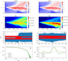 |
Fig. 1. Upper half: density and energy (in eV) distributions of electrons (a,c) and protons (b,d) at t = 140 Ω−1 for mi/me = 100, n0 = 1012 m−3. The magnetic field B0 = 10−3 T, By/B0 = 0.1, Bx/B0 = 0.02, and electric field E0 = 250 V m−1. Lower half: Vz vs x distributions in the velocity phase space for (e) n0 = 108 m−3 and (f) 1012 m−3. (g) and (h) compare the energy spectra and the polarisation electric field Ex vs x at |

The PIC simulations of particle acceleration in a low-density current sheet reproduce the similar results obtained from test-particle simulations, as the asymmetry of electrons and protons at ejection from the midplane is clear in the velocity phase space (Fig. 1e) (Siversky & Zharkova 2009; Xia & Zharkova 2018). For higher ambient plasma density, the newly obtained particle density and energy distributions reveal noticeable differences from the test-particle approach where the asymmetry of ejected protons and electrons is more distinguishable in the energy distributions (Figs. 1c,d) rather than in the density distributions (Figs. 1a,b).
Another important outcome of this charge separation of accelerated particles is the induction of the polarisation electric fields  and additional fluctuations in PIC simulations. The induced
  is mainly perpendicular to the RCS midplane and it becomes larger when the ambient plasma density increases (Fig. 1h). It is larger than
  and
and  by an order of magnitude, which is close to the previous estimations (see also Zharkova & Gordovskyy 2004; Zenitani & Hoshino 2008; Cerutti et al. 2013).
2.2.2. Transit vs bounced particles
There is also a distinction between the dynamics of particles of the same charge entering a reconnecting current sheet from opposite edges. Namely, the particles entering the current sheet from the same side, to which they are to be ejected, are classified as “bounced” particles; the particles entering the CS from the opposite side, to which they are to be ejected, are classified as “transit” particles. The transit electrons gain much higher energies and form the power-law tail of energy spectra while the bounced electrons gain much smaller energies and often have a quasi-thermal wide spectrum (Fig. 1g). In fact, accelerated electrons in Fig. 1 are split into two distinct groups in energy: the low-energy bounced electrons (with the energies <300−500 eV) and high-energy transit electrons (with energies up to keVs). The value of the threshold depends on the magnetic field magnitude as it is higher for stronger magnetic field strength. This is caused by transit (bounced) electrons gaining (losing) their energy while reaching the midplane where the main acceleration occurs. The uneven distributions of transit and bounced particles across the midplane, well distinguishable in TP approach, are harder to notice in the velocity phase space for PIC simulations (Fig. 1f) because of the polarisation electric field.
As a result of this different particle dynamics while moving through a current sheet, the overall energy distributions of accelerated electrons/protons would have two maxima or a “bump-on-tail” for transit particles. It can generate turbulence in the vicinity to the X-nullpoint owing to Buneman instability (Buneman 1958), which is not accessible with the previous test-particle approach. As shown in Figs. 2 and 3, the fluctuations propagate along z- and y-directions rather than along the x-direction. The Ez component representing Langmuir waves oscillates at ≈1.3 × 10⁻⁷ s, which is close to the plasma frequency for the plasma density of 1012 m3 accepted in this simulation (Drake et al. 2003; Siversky & Zharkova 2009). Because the gradient of  is mainly along x-axis (Fig. 2), then following Faraday’s law, the variations of
  do not induce a noticeable change of the magnetic fields in this region. In addition to the background static fields, the fluctuations of the induced magnetic field components
  ,
,  ,
,  are measured to be < 1.0 × 10⁻⁴ from the simulations (Fig. 2).
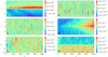 |
Fig. 2. Changes of electric and magnetic fields in the simulation (n0 = 1010 m−3): left column: x, y, z components of |


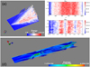 |
Fig. 3. Upper plot (a): x−z cut (the front plane) and the isosurface (behind the plane) of the electron energy at t = 1500 Ω−1 in the 3D simulation. Upper right plots: (b) corresponding picture on the y−z plane at x = 0, (c): contour on the x−y plane at z = 960. The parameters are By/B0 = 0.1, Bx/B0 = 0.02, B0 = 10−3 T, and E0 = 250 V m−1. Bottom panel (d): isosurface of the proton energy in the whole simulation domain including the x−z cut at y = 0 (Parameters and more details are explained in the next Sect. 3.2.1). |
Proton beams were also shown to generate other turbulence at some distance from X-nullpoints (see Drake et al. 1994; Shay et al. 1998; Liu et al. 2012; Zhang et al. 2019, for more details). However, in the current simulations, we only can detect the waves with wavelengths shorter than the size of the simulation domain. Further investigation of the turbulent wave generation by particles accelerated in current sheets will be carried out in the forthcoming paper.
2.2.3. Comparison of 2.5D and 3D simulations
Furthermore, we inspect the differences in particle distributions between the 2.5D (Fig. 1) (solving 3D motion equations for velocity in 2D Cartesian coordinates (X and Z)) and full 3D (where the variation in the Cartesian coordinate Y is added) simulations with the relativistic 3D PIC simulation code, VPIC (Bowers et al. 2008) (Figs. 3a–c). In order to compare to so, we carried out 3D simulations in the region with the same parameters as the 2.5D version. The out-of-plane length Ly equals to the thickness Lx, and the boundaries at y = 0, Ly are set to be periodic).
Although there are some fluctuations along the y-axis in 3D simulations, as shown in Figs. 3b,c, the density and energy distributions in the x−z plane are similar to those obtained in 2.5D simulations as shown for a few slices at different y, so for the whole domain. Moreover, any fluctuations of particle distributions and electromagnetic fields along the y-direction in 2.5D and 3D PIC simulations being a consequence of kink instability out of the reconnection plane are found suppressed by the embedded static magnetic field with strong guiding field described in Sect. 2.1 (for more details, see Lapenta & Brackbill 1997; Daughton 1999; Cerutti et al. 2014; Sironi & Spitkovsky 2014, and references therein). Then the similar outcomes of particle distributions in 2.5D and 3D are not surprising because they do not have any differences in the 3D velocity space from the start, as we explained in the first paragraph. Thus, from now on, to make our statements in 3D cases, we only show the distributions of the particle variables on the x−z plane.
2.2.4. The pitch-angle distributions
The unique property of the PIC approach allows us to derive pitch-angle distributions of particles at ejection from a current sheet. In this step, we carry out 3D PIC simulations in the region with periodic boundary conditions to both the electromagnetic fields and particle motion in the z-direction following Siversky & Zharkova (2009). As we established in Sect. 2.2.1, the effect of magnetic field topology on particles of the same charge entering the reconnecting current sheet from opposite sides leads to very different energy gains by transit and bounced particles. It turns out that it also changes the locations where these particles are ejected from the current sheet, or different pitch-angle distributions at ejection.
In the magnetic topology without any guiding field, the plot of Vz vs x and the pitch-angle distributions shown in Figs. 4a1–a4 are quite symmetric with respect to the midplane, x = 0, because the magnetic field topology does not impose any separation by charge. When the low-energy electrons drifting along the midplane, they tend to move quasi along the magnetic field component Bz and, thus, form the pitch-angle distribution towards 0° in x > 0 and 180° in x < 0 semi plane due to the magnetisation (note that B is along −z axis for x > 0 and along +z axis for x < 0). After acceleration, low-energy particles would turn away from the midplane and move anti-parallel to the drifting-in particles (see Fig. 1). Thus, the pitch-angle distributions of low energetic electrons peak near 180° to the Bz component in x > 0 and 0° in x < 0 semi plane in Fig. 4a2. While high-energy particles would move across the midplane in the parallel direction to drift-in particles, as they would have pitch angles peaking at 0° in Fig. 4a3. Therefore, the bidirectional flows of highly energetic particles seen in the heliosphere (Zharkova & Khabarova 2015) can be these distributions of high-energetic electrons ejected from the different quarters of an RCS occurred at the front of ICME.
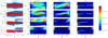 |
Fig. 4. Vz vs x distributions in phase space and the pitch-angle distributions for By/B0 = 0 (a-first row), 0.1 (b-second row), 1.0 (c-third row), and 1.0 with d = 10 (d-fourth row): in each row, Vz vs x of electrons (blue dots) and protons (red dots) (first column), the pitch-angle distribution of low-energy electrons (second column), the pitch-angle distribution of high-energy electrons (third column), and the pitch-angle distribution of protons (fourth column) are presented from left to right for each individual By/B0 ratio. The current sheet parameters are B0 = 10−3 T, E0 = 250 V m−1, and d = 1 for (a–c). The magnetic field topology in the reconnection plane is similar to that of Fig. 1. |
With the addition of a noticeable guiding field By, the asymmetry of accelerated particles about the midplane is increased as revealed by their pitch-angle distributions. The transit electrons (protons) become more dominant in the x > 0 (x < 0) semi planes in Figs. 4b3, c3 (and b4, c4 for protons) in the low-energy channel near 180° (0° for protons). Correspondingly, the dispersion of the pitch-angle distribution decreases in another semiplane, the high-energy particles become focused about a particular direction. Furthermore, in moderate guiding field transit electrons are also shown in the low-energy channel near 180° as shown in Fig. 4c2 as they are ejected from the midplane similar to the bounced low-energy electrons as demonstrated in Fig. 1. When the guiding field is very strong, e.g. By/B0 = 1.0, the accelerated electrons and protons are fully separated, the pitch-angle distributions of the oppositely charged particles show a strong asymmetry that can be seen from Figs. 4c2 and c3.
When a current sheet becomes thicker, the transit electrons gain more energy during acceleration as shown for d = 10 in Fig. 4d1. On the other hand, when the magnetic field becomes weaker and the current sheet becomes thicker, like in the heliospheric current sheet (HCS), the bounced electrons could not reach the midplane. This is because they become fully magnetized by the guiding field and, thus, turn around by 180° well before they reach the midplane. Therefore, in this scenario the locations where electrons reverse their pitch-angles do not match with the midplane of the RCS as they are expected in a thin current sheet with a weak guiding field.
This asymmetry of accelerated particles and their pitch-angles during passing through reconnecting HCS can explain some unusual pitch-angle observations of energetic particles turning away well before the magnetic field reversals in the sector boundaries (Crooker et al. 2004), as Fig. 4 confirms the explanation proposed by Zharkova & Khabarova (2012). Therefore, the pitch-angle distributions obtained here can be further compared with available observations of electron pitch-angle spectrograms (Khabarova et al. 2015) taken from in-situ observations in the heliosphere, which will be the topic of the forthcoming paper (Khabarova et al., in prep.).
3. Particle acceleration in an RCS with magnetic islands
In this section, we consider particle acceleration using 2.5D and 3D PIC approaches in the reconnecting current sheets, which are broken into magnetic islands. Similar to the previous studies (Xia & Zharkova 2018), let us explore two types of magnetic islands: squashed magnetic islands, or contracting islands, where the plasma flows into the islands from all directions (Drake et al. 2006b; Oka et al. 2010), and coalescent magnetic islands, or merging islands, that the two islands move towards one another (Pritchett 2008; Wan & Lapenta 2008; Werner et al. 2017). The current sheets with magnetic islands have a similar thickness of dcs = 2 as considered for RCSs with a single X-nullpoint in Sect. 2.1. The electrons and protons are injected into the simulation domain from both boundaries, which are located at a distance L = ±10 away from the midplane of the CS.
3.1. Background
The initial magnetic fields are accepted to follow those considered in the test-particle studies (Xia & Zharkova 2018):
 (5)
(5)
 (6)
(6)
 (7)
(7)
where dcs is the half thickness of RCS near the O-nullpoint, ξy is the parameter of the guild field ratio as in Eq. (1), and ϵ, k are the mathematical parameters controlling the dimension of the periodic islands. k = Li/dcs is the ratio of the half length of the island Li, to the current sheet half thickness dcs. This model describes a series of identical islands periodically occurring along the x = 0 plane in the current sheet.
The reconnection electric field Ey is determined by the ambient plasma inflow velocity and the reconnection magnetic field magnitude (Jaroschek et al. 2004). In the squashed magnetic islands, the static reconnection electric field can be described as (Kliem 1994),
![Mathematical equation: $$ \begin{aligned} E_{y,\mathrm{s}}= E_{0} [0.6 + 0.4 \cos (k z/d_{\rm cs})]. \end{aligned} $$](/articles/aa/full_html/2020/03/aa36420-19/aa36420-19-eq31.gif) (8)
(8)
Another type of magnetic islands, the coalescent islands, are represented by the static reconnection electric field (Li & Lin 2012),
 (9)
(9)
The reconnecting electric field Ey, c and the plasma flow direction are presented in Fig. 5, in which the parameters used are k = 0.0325, ϵ = 0.3, d = 2, and E0 = 100 V m−1. The half length of magnetic islands is thus Li = 64 along the midplane of the RCS. For our magnetic islands study, the simulation domain is restricted to the box region in Fig. 5 (upper plot), where the geometry of the magnetic islands is open at both ends of the simulation domain. Thus, there is a pair of closed coalescent magnetic islands near z = 384, while the particles can escape the chain of magnetic islands near z = 0, 512 in the bottom panel of Fig. 5.
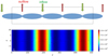 |
Fig. 5. Upper plot: scheme of coalescent magnetic islands and plasma flow direction. Bottom plot: amplitude of reconnection electric field Ey, c (V m−1 in the colorbar) from Eq. (9) generated in islands. The parameters for Ey, c are k = 0.0325, ϵ = 0.3, d = 2, and E0 = 100 V m−1. |
3.2. Simulation results
3.2.1. Particle separation in coalescent magnetic islands
The first simulation of coalescent magnetic islands is schematically shown in Fig. 5 (top panel) with relevant reconnection electromagnetic fields in the bottom panel. The particle density and energy distributions in two coalescent islands are plotted in Fig. 6 at t = 560 Ω−1, when the maximal particle energies are observed. The particle density and energy distributions show a clear asymmetry with respect to the midplane (indicated by the arrows in Fig. 6) due to the guiding field By, which is similar to that reported for particles moving around a single X-nullpoint. For example, near the fully opened boundaries (z < 130 and > 480 marked by purple arrows), the high-energy electrons are moving to the opposite half plane (see Figs. 6a,c) against the high-energy protons (see Figs. 6b,d). Thus, the preferential ejection phenomenon is validated for coalescent islands.
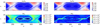 |
Fig. 6. Density and energy distributions of particles in the coalescent magnetic islands at |

In general, the particle energy gains in the islands are higher and achieved on shorter spatial scales than those near the single X-nullpoint obtained with the current PIC simulations. This point is discussed in more details below in Sect. 3.2.4. Considering that the magnetic topologies for single and multiple X-nullpoints have the similar electromagnetic field parameters and overall sizes, this suggests that within the current sheets of similar dimensions the particles are accelerated more efficiently in magnetic islands than near a single X-nullpoint. As the simulation evolves, the magnetic field topology is changed significantly since the magnetic islands are merging (similar to that shown in Fig. 1 in Pritchett 2008). Hence, at a later time, there is a decrease in high-energy particle numbers in the islands, indicating that high-energy particles have escaped the magnetic islands through the open boundaries.
3.2.2. Polarisation electric field in coalescent magnetic islands
A change of the magnetic island topology from a single X-nullpoint to coalescent magnetic islands also changes the polarisation electric field induced by accelerated particles. As the particle separation still occurs in magnetic islands as shown Sect. 3.2.1, so should the polarisation electric field,  , induced by the separated particles. Similar to the
  component for a single X-nullpoint shown in Fig. 1, the amplitude of
  in magnetic islands shown in Fig. 7 is larger than the reconnecting electric field E0 (100 V m−1), although the enhancement of
  is smaller than the one generated near a single X-nullpoint in Fig. 2.
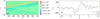 |
Fig. 7. Polarisation electric field Ex from the simulations previously presented in Fig. 6: (a) map of Ex in the open field region z > 445, (b) values of Ex across the midplane for different z in the left contour. |
Another property of  in RCS with a single X-nullpoint is switching the sign near the midplane, as shown in Figs. 2a and 1b. However, in the coalescent magnetic islands considered here,
  switches its sign along the separatrix of the open field region as indicated by the edge between blue and red colours in Fig. 7a. More specifically, Fig. 7b shows that
  changes its sign near x = 0 in the z = 445 plane, then in the downstream at z = 470,
  changes sign near x = 2.0 in this case. Thus, the polarisation electric field is extended beyond the diffusion region midplane.
3.2.3. Squashed magnetic islands
Let us consider another type of magnetic islands, that is, squashed ones, by replacing the electric field of coalescent magnetic islands described in Sect. 3.2.1 with the one relevant to the squashed magnetic islands. We keep the z- and x-boundaries open as in coalescent islands. The results are shown in Fig. 8. Here we should mention that preferential ejection caused by the guiding magnetic field and induced polarisation electric field are also presented in the open magnetic field region of squashed magnetic islands, similar to the coalescent ones shown in Fig. 6. Although, in this topology, the asymmetric particle distributions in the open field region in Figs. 8c and d are not so evident because at this time these particles are mainly engaged in the acceleration inside the islands that only a small part of particles gain the sufficient energy to escape through the exhausts. Thus, the densities of escaping particles are much lower than the ones in the middle of the islands as it was confirmed by the further study of the local open-field region like Fig. 7 (not shown in the figures).
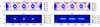 |
Fig. 8. Energy distribution of particles in squashed magnetic islands at |

By comparing Fig. 8 with Fig. 6 obtained after the same simulation time for coalescent magnetic islands, it shows that the energy gains by particles are noticeably higher (by a factor of 6 or larger) in squashed islands. This can be explained by the difference between the electric fields of the squashed and coalescent islands (see the model descriptions in Eqs. (8) and (9)). Namely, the merging area of coalescent islands has Ey < 0, which is antiparallel to the reconnecting electric field, while the resulting electric field remains all positive across the whole domain when a magnetic island becomes squashed.
Therefore, the energy gains of particles in the squashed island are much higher than in the coalescent island that has the same initial magnetic field geometry, as explained in Sect. 3.2.2. This is close to the result reported from the test-particle study (Xia & Zharkova 2018). Furthermore, we notice that the energetic particles are confined in the centre and midplane of the squashed islands, while they circle about the X-nullpoints in the coalescent islands. A more detailed analysis of the particle energy gains in the two types of magnetic islands is discussed later in Sect. 4.2.
3.2.4. Energy spectra of electrons in magnetic islands
Within the same type of magnetic islands, whether coalescent or squashed, the variation of the parameters, such as the guiding field strength and the aspect ratio of the length-to-thickness, would the energy spectra as shown in Fig. 9. The energy gains by electrons are enhanced in the elongated magnetic islands (the curve “Ck2”: k = 0.015625), and when the guiding magnetic field increases (“CBy”: By/B0 = 1). The variation of the proton-to-electron mass ratio does not change much the energy spectra of accelerated electrons for the same magnetic field topology, only affecting the maximum energy gains (e.g. in comparing the curves “Cm1”, “C”, “Cm2” in Fig. 9). Besides, there are more energetic electrons produced in the squashed magnetic islands (“S”) than in the coalescent magnetic islands (“C”) that makes the spectrum in squashed islands harder as it was already mentioned in Sect. 3.2.3.
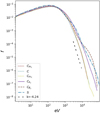 |
Fig. 9. Energy spectra of electrons in the simulations which have been presented in Figs. 6 (“C”) and 8(“S”). “Cm1” and “Cm2” come from the 2.5D simulations with mi/me = 10.0 and mi/me = 200.0 using the same RCS parameters as the one in Fig. 6. The simulations of “Ck2” and “CBy” have different k( = 0.015625) and By(By/B0 = 1) from the one in Fig. 6. The dashed line represents a referential spectral line ∼E−4.2. |
Furthermore, energy gains by transit electrons are much higher than by bounced ones, dividing the populations of energetic electrons by the threshold energy of 300−500 eV for bounced and up to hundred keV energies for transit electrons. This leads to a bump-on-tail energy distribution of accelerated particles (“CBy”), which is similar to the electron spectrum in the single X-nullpoint simulation shown in Fig. 1d for the same particle inflow density of 1012 m−3. As a result, this would lead again to Buneman instability and formation of turbulence within a short time between the neighbouring magnetic islands, thus, partially obscuring their periodic structure as reported in 3D simulations by Daughton et al. (2011).
Our results vary from some other PIC simulations because we use the open boundary condition allowing particles to leave the simulation domain, while in the other PIC studies periodic or reflecting boundary conditions are applied (Drake et al. 2006b; Guo et al. 2014). This introduces a particle loss mechanism, which would change the energy spectrum (Zenitani & Hoshino 2001; Drake et al. 2010, 2012; Guo et al. 2014). One may also note that the spectra of electrons found in the PIC simulations are much softer than those derived for the same conditions in the TP studies (Xia & Zharkova 2018), except that high-energy particles could escape from the open boundary, where the variable electric fields induced by accelerated particles, like the polarisation one, still change the magnetic field and thus affect the acceleration time and energy gains of particles while they are confined within the islands, as mentioned in Sects. 3.2.2 and 3.2.3.
4. Evaluation of energy gains in magnetic configurations
4.1. General comments
It has been well established that particles in magnetic reconnection are firstly accelerated by a reconnection electric field, while magnetic field topology plays a very important role by keeping the particles within a magnetic configuration, thus, making them gain more energy. Acceleration in reconnecting current sheets with a single X-nullpoint has been extensively investigated over the past decade. It was established the accelerated particles gain power-law energy spectra, whose parameters depend on magnetic field component ratios (Zharkova et al. 2011). It was also found that particles of the opposite charges are ejected from a current sheet into the opposite directions from the current sheet midplane, which induces a strong polarisation electric field. However, this approach also uncovered a hidden problem for particle acceleration given that it requires pretty long thin current sheets to be stable during the whole acceleration process. Often this condition cannot be fulfilled, so it imposes a serious problem for the generation of the observable amount of accelerated particles.
MHD and full kinetic simulations of magnetic reconnection have shown that long current sheets are often affected by tearing instabilities leading to the formation of magnetic islands (Loureiro et al. 2005; Bárta et al. 2011; Drake et al. 2006a; Huang & Bhattacharjee 2010; Karimabadi et al. 2011; Nishizuka et al. 2015). The motion of the islands is self-controlled by the reconnection process and the plasma feedback due to the presence of accelerated particles. The islands, in turn, are rather dynamic, which can be growing or squashed in different dimensions and even merging with each other at all time. The question is how particle acceleration would be changed in these dynamic magnetic islands conditions and how these changes would feedback to electromagnetic fields by accelerated particles, which we attempt to answer in this study.
As we established in Sects. 3.2.1 and 3.2.2 above, the adopted models describe the topology of magnetic field lines and relevant plasma flows of the chains of coalescent and squashed magnetic islands (Kliem 1994; Li & Lin 2012; Zhang et al. 2014; Li et al. 2017). For simplicity, in many transport models the particles are often considered surfing through a bunch of magnetic islands where they are accelerated through different energisation processes (Zank et al. 2014; le Roux et al. 2015). In order to understand the links between the particle energisation mechanisms suggested in transport equations using the guiding centre approach (le Roux et al. 2015), let us investigate particle acceleration in a chain of magnetic islands by the following acceleration mechanisms: the magnetic curvature, gradient drift, and parallel electric field using the PIC approach.
4.2. Estimations of the energy gains
To understand the particle acceleration during magnetic reconnection, we adopt the guiding-centre drift approach (Drake et al. 2006b; le Roux et al. 2015; Li et al. 2018) to explore the contributions of each acceleration mechanism related to particle drift motions in the RCSs with coalescent and squashed magnetic islands. The energy gain of particle s (carrying a current js) coming from js ⋅ E (Parker 1957) could be split into parallel and perpendicular components (with respect to the local magnetic field component):
 (10)
(10)
where in PIC simulations the parallel electric field E∥ is mainly induced by accelerated electrons, and the perpendicular component E⊥ comes from the reconnecting electric field, electron pressure tensor, instabilities (Jaroschek et al. 2004) and the polarisation electric field considered in Sect. 3.2.2 above (Hesse et al. 2001). The vector js is also split between the parallel and perpendicular directions with respect to the local magnetic field line.
On the other hand, the momentum conservation equation can be written as
 (11)
(11)
where ps is the momentum density, Ts is the stress tensor, ρs is the charge density, and B is the magnetic field. With some algebra by averaging the particle gyromotion (le Roux et al. 2015; Li et al. 2018), the perpendicular component of js can be expressed as
![Mathematical equation: $$ \begin{aligned} \boldsymbol{j}_{\rm s\perp } =&\boldsymbol{j}_{\rm c} + \boldsymbol{j}_{g} + \boldsymbol{j}_{\rm m} + \boldsymbol{j}_{{\boldsymbol{E}}\times \boldsymbol{B}} +\boldsymbol{j}_{p} \nonumber \\ =&p_{\rm s\parallel }\frac{{\boldsymbol{B}}\times (\boldsymbol{B}\cdot \nabla )\boldsymbol{B}}{B^4} + p_{\rm s\perp } \frac{{\boldsymbol{B}}\times \nabla B}{B^3} + \left[-\nabla \times \frac{p_{\rm s\perp }\boldsymbol{B}}{B^2}\right]_\perp \nonumber \\& + \rho _{\rm s} \frac{{\boldsymbol{E}}\times \boldsymbol{B}}{B^2} + \rho _{\rm s} \frac{{\boldsymbol{B}}}{B^2}\times \frac{\mathrm{d} \boldsymbol{u}_{\rm s}}{\mathrm{d}t}, \end{aligned} $$](/articles/aa/full_html/2020/03/aa36420-19/aa36420-19-eq45.gif) (12)
(12)
where the first two leading terms (jc, jg) on the right side describe the energy gains owing to the magnetic curvature drift and gradient drift respectively, with the other contributions coming from magnetisation (jm), E × B (jE × B), and polarisation drift (jp) are proved to be relatively small (Dahlin et al. 2015; Li et al. 2018).
The results of simulations shown in Fig. 10 include the spatial distributions of je∥E∥, jcE⊥, and jgE⊥ for electrons in different magnetic islands. The distributions of various energisation terms in the squashed islands (Figs. 10d–f) are quite different from the ones in coalescent islands (Figs. 10a–c). The difference comes from the evolution of particle motion in magnetic islands and this is not expected at the beginning from Eqs. (8) and (9).
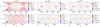 |
Fig. 10. Distributions of the energisation terms, j∥E∥, jcE⊥, and jgE⊥ in Eqs. (10) and (12) for coalescent (upper panels a–c) and squashed magnetic islands (bottom panels d–f). The colorbar indicates the amplitudes. The corresponding electron distributions can be found in Figs. 6 and 8. |
In both types of magnetic islands, the contribution from je∥E∥ is smaller than the others, and it is mainly located near the outer shells of the magnetic islands, similar to that shown in Figs. 6 and 8. Hence, the parallel electric field is carried by accelerated electrons and thus cannot accelerated particles further. The main contribution to particle acceleration in both types of islands comes from jcE⊥, and it is larger in squashed islands. Although jgE⊥ and the energetic particles are confined near the midplanes of O-nullpoints in the squashed islands while they only peak near the X-nullpoints in coalescent islands, which has not been discovered in the previous test-particle studies. Meanwhile, the distribution of jgE⊥ term is similar to the one of jcE⊥, but the amplitude of the former is smaller than the latter. The contribution from jgE⊥ could be negative in more regions in the coalescent islands, which means a cooling effect can be expected instead of acceleration (Bessho & Bhattacharjee 2012).
In comparing Figs. 6 and 8, we found that the distributions of energisation terms match closely the energy distributions of particles in both island topologies. This indicates that the jcE⊥ and jgE⊥ are responsible for providing the energetic particles along the midplane, X-nullpoints and cores of squashed islands, and the extensions (separatrices) from the X-nullpoints. The je∥E∥ contributes to the particle energisation along the separatrices and the outer areas surrounding the magnetic islands.
The large amplitude of jcE⊥ in squashed islands thus explains why particle acceleration is more efficient in squashed islands rather than in the coalescent ones. This result obtained in the present PIC approach supports the analytic conclusion from Zank et al. (2014). Meanwhile, we notice that both the pile-ups of energetic particles in the cores of squashed islands (away from the X-nullpoints) and surrounding the coalescent islands have been separately reported in relativistic magnetic reconnection studies (Zenitani & Hoshino 2007; Sironi & Spitkovsky 2014; Nalewajko et al. 2015). It suggests that the sampled magnetic islands are dominated by different motions, merging or contracting, which may need to be considered in future works.
5. Discussion and conclusions
In this paper, we investigate particle acceleration in non-relativistic reconnecting current sheets (RCSs) with different magnetic topologies using a collisionless PIC approach. The ambient plasma dragged into a current sheet by the magnetic diffusion process associated with magnetic reconnection are studied in a small part of the RCS with a 3D magnetic field configuration. In this study, the background electric and magnetic fields produced by magnetic reconnection on a magnetohydrodynamic scale are considered to be stationary. Then particle trajectories inside reconnection regions are calculated by the 3D PIC simulations, which also calculate the ambient plasma feedback, for example, the electric and magnetic fields generated by accelerated particles themselves. In the current models, the use of the static background fields including the guiding field helps to suppress the occurrence of kink instability along y-direction in 3D simulations. Thus, it is not surprising that the generated density and energy distributions of particles are similar in the presented 2.5D and 3D simulations as they start with the same distributions in 3D velocity space. This conclusion is similar to the previous studies of magnetic reconnection, which investigated the change of reconnection rates and particle acceleration in 3D reconnecting current sheets (Hesse et al. 2001; Zeiler et al. 2002; Drake et al. 2003; Liu et al. 2011; Guo et al. 2014; Dahlin et al. 2017).
The simulations were first benchmarked by the particle dynamics in the vicinity of a single X-nullpoint. This confirmed that in a current sheet with a strong guiding field, the oppositely-charged energetic particles are separately ejected from the RCS with respect to the midplane, e.g., for a given magnetic topology electrons can be ejected into the positive x-semiplane and protons into the negative x-semiplane from x = 0. This asymmetry produces a polarisation electric field  across the midplane, which governs the further particle motions inside an RCS (Zenitani & Hoshino 2008; Siversky & Zharkova 2009).
Moreover, particles of the same charge were found to also have asymmetric trajectories and energy gains depending on the side, from which they are dragged into the current sheet. The “transit” particles, which move across the current sheet midplane, gain more energies during their drift towards the midplane where the main acceleration occurs. The “bounced” particles, which are ejected from the same side of the current sheet where they enter, lose their energy during the drift-in phase. This creates two distinguished populations of energetic particles with significantly different energies that could be detected by in-situ observations in the heliosphere or magnetosphere.
The transit and bounced particles ejected to the same side of the current sheet form the energy spectra with two maxima, or bump-on-tail distributions, leading to the formation of plasma turbulence close to the edge of the current sheet (Jaroschek et al. 2004; Siversky & Zharkova 2009). More significantly, “transit” and “bounced” electrons can produce rather distinguishable narrow pitch-angle distributions (unidirectional beams centred near 0° or 180°), while moving either parallel or antiparallel to the local magnetic field lines at the ejection sides. Owing to a significant difference in energy gains between transit and bounced ones, the pitch-angle distribution of electrons in high energy channel (with energies ≥300−500 eV) is different from the one in the lower energy channel (≤300−500 eV). Low-energy electrons tend to move along the magnetic field lines not approaching current sheet midplane, and to form a peculiar pitch-angle distribution in the opposite direction where they were dragged in, e.g., with the pitch-angles centred about 180° from the Bz-component. While energetic electrons are mainly ejected in the same directions where they were dragged into, e.g. centred about the pitch-angles of 0° from the Bz-component. Furthermore, the energetic transit electrons dragged into the whole current sheets form the bidirectional energetic beams moving in the opposite directions: e.g. in the positive semi-plane from the midplane (X > 0) with pitch angles of 0° from the Bz-component and in the negative semi-plane from the midplane with pitch-angles of 180° from the Bz-component.
This difference in pitch-angle distributions is often observed in the current sheets occurring at the front edge of ICMEs (Zharkova & Khabarova 2015), where the asymmetric high-energy electrons (“strahls”) are often detected moving perpendicular to the interplanetary magnetic field in the opposite directions from the two current sheet exhausts. Our current results showing the asymmetric pitch-angle distributions across different energy channels can be observed in the pitch-angle spectrograms in the heliosphere that will comprise the scope of a forthcoming paper.
We also considered with PIC approach particle acceleration in 3D current sheets with two typical magnetic islands: coalescent and squashed islands. Unlike other models of particle acceleration, our approach distinguishes the static background electromagnetic fields coming from the magnetohydrodynamic scale from the ones induced by accelerated particles themselves because of the plasma feedback. Also, we considered the coalescent (merging) and squashed (contracting) motion of magnetic islands are predefined rather than generated from the perturbed Harris sheet in a closed system.
It was established that, similarly to the studies in RCSs near a single X-nullpoint, the increase of a guiding field in the RCS with multiple X- and O-nullpoints also leads to the increases of particle energy gains in magnetic islands. If current sheets have comparable dimensions, the ones with magnetic islands are shown to be more efficient on accelerating particles to higher energies than the ones with a single X-nullpoint. Furthermore, like particle acceleration near a single X-nullpoint, there is a preferential ejection of oppositely charged particles close to the exhausts of magnetic islands with open boundaries, which are characterised by the accumulation of high energetic particles at these locations. The polarisation electric field induced by accelerated particles in magnetic islands is also present, in general, close to the separatrices near the open boundaries being slightly lower than in current sheets with a single X-null point (see also Zenitani & Hoshino 2008; Markidis et al. 2012; Cerutti et al. 2013).
The spatial distributions of the particle energy distributions show that particle acceleration in squashed islands is more effective than in the coalescent ones, which is also confirmed by the energy spectra. The results verified that particle acceleration in squashed islands is more effective than in the coalescent ones as it has been previously estimated (Zank 2014). Moreover, the contracting motion of squashed magnetic islands is shown to pile up the particles in the middle of O-nullpoint. While the coalescent motion accumulates the energetic particles near X-nullpoints surrounding the islands, which reproduces the result of the previous relativistic magnetic reconnection study (Nalewajko et al. 2015).
Besides, the energy spectra of electrons in varies magnetic islands show that the magnetic island geometry, such as the aspect ratio of its length to width, affect the energy gains of particles. Meanwhile, the increase of the proton-to-electron mass ratio does not change the energy spectra of accelerated electrons but only increases the maximal energy gain. In summary, the energy spectra of particles accelerated in the presented magnetic islands have a spectral index ∼−4.2 for coalescent islands and −4.0 for squashed islands, which are both softer than the index ≈(−1.2, −2.4) obtained in the similar islands from the test-particle approach (Ripperda et al. 2017). This is understood in terms of the electromagnetic fields induced by the plasma feedback in PIC to the presence of accelerated particles And the open boundary condition allowing high-energy particles to leave the islands softens the energy spectrum (Birn et al. 2017).
The difference between particle acceleration in coalescent and squashed islands is also analysed by examining the particle drift motions and benchmarking to the picture of particle transport in multiple magnetic islands (Zank et al. 2014; le Roux et al. 2015). It has been established that the main contribution to particle energisation in magnetic islands comes from the perpendicular direction, more specifically, from the particle magnetic curvature drift along the electric field, which is associated with the Fermi reflection at both ends of contracting magnetic islands (Dahlin et al. 2014; Ball et al. 2018).
Therefore, we can conclude that the magnetic field topology in current sheets with multiple X- and O-nullpoints plays an important role in particle acceleration defining the specific energy and pitch-angle distributions for particles passing through reconnecting current sheets in the solar and space plasmas. This characteristics of accelerated particles can be identified from in-situ observations, which will comprise the scope of a forthcoming paper.
Acknowledgments
The authors wish to thank the referee for providing very helpful comments, from which the paper strongly benefited. The authors acknowledge the funding for this research provided by the US Air Force grant PRJ02156. This work used the DiRAC Complexity system, operated by the University of Leicester IT Services, which forms part of the STFC DiRAC HPC Facility (www.dirac.ac.uk). This equipment is funded by BIS National E-Infrastructure capital grant ST/K000373/1 and STFC DiRAC Operations grant ST/K0003259/1. DiRAC is part of the National e-Infrastructure.
References
- Angelopoulos, V., McFadden, J. P., Larson, D., et al. 2008, Science, 321, 931 [NASA ADS] [CrossRef] [Google Scholar]
- Ball, D., Sironi, L., & Özel, F. 2018, ApJ, 862, 80 [NASA ADS] [CrossRef] [Google Scholar]
- Bárta, M., Büchner, J., Karlický, M., & Skála, J. 2011, ApJ, 737, 24 [NASA ADS] [CrossRef] [Google Scholar]
- Battaglia, M., & Kontar, E. P. 2012, ApJ, 760, 142 [NASA ADS] [CrossRef] [Google Scholar]
- Baumann, G., & Nordlund, Å. 2012, ApJ, 759, L9 [NASA ADS] [CrossRef] [Google Scholar]
- Benz, A. O. 2017, Liv. Rev. Sol. Phys., 14, 2 [Google Scholar]
- Bessho, N., & Bhattacharjee, A. 2012, ApJ, 750, 129 [NASA ADS] [CrossRef] [Google Scholar]
- Birn, J., & Priest, E. R. 2007, Reconnection of Magnetic Fields: Magnetohydrodynamics and Collisionless Theory and Observations (Cambridge: Cambridge University Press) [CrossRef] [Google Scholar]
- Birn, J., Battaglia, M., Fletcher, L., Hesse, M., & Neukirch, T. 2017, ApJ, 848, 116 [NASA ADS] [CrossRef] [Google Scholar]
- Boris, J. P. 1970, Proceeding of Fourth Conference on Numerical Simulations of Plasmas (Washington DC: Naval Research Laboratory) [Google Scholar]
- Bowers, K. J., Albright, B. J., Yin, L., Bergen, B., & Kwan, T. J. T. 2008, Phys. Plasmas, 15, 055703 [NASA ADS] [CrossRef] [Google Scholar]
- Buneman, O. 1958, Phys. Rev. Lett., 1, 8 [NASA ADS] [CrossRef] [Google Scholar]
- Cerutti, B., Werner, G. R., Uzdensky, D. A., & Begelman, M. C. 2013, ApJ, 770, 147 [NASA ADS] [CrossRef] [Google Scholar]
- Cerutti, B., Werner, G. R., Uzdensky, D. A., & Begelman, M. C. 2014, ApJ, 782, 104 [NASA ADS] [CrossRef] [Google Scholar]
- Chen, L.-J., Bhattacharjee, A., Puhl-Quinn, P. A., et al. 2008, Nat. Phys., 4, 19 [CrossRef] [Google Scholar]
- Chian, A. C.-L., & Muñoz, P. R. 2011, ApJ, 733, L34 [NASA ADS] [CrossRef] [Google Scholar]
- Crooker, N. U., Huang, C. L., Lamassa, S. M., et al. 2004, J. Geophys. Res.: Space Phys., 109 [Google Scholar]
- Dahlin, J. T., Drake, J. F., & Swisdak, M. 2014, Phy. Plasmas, 21, 092304 [NASA ADS] [CrossRef] [Google Scholar]
- Dahlin, J. T., Drake, J. F., & Swisdak, M. 2015, Phy. Plasmas, 22, 100704 [NASA ADS] [CrossRef] [Google Scholar]
- Dahlin, J. T., Drake, J. F., & Swisdak, M. 2017, Phys. Plasmas, 24, 092110 [NASA ADS] [CrossRef] [Google Scholar]
- Daughton, W. 1999, Phys. Plasmas, 6, 1329 [NASA ADS] [CrossRef] [Google Scholar]
- Daughton, W., Roytershteyn, V., Karimabadi, H., et al. 2011, Nat. Phys., 7, 539 [NASA ADS] [CrossRef] [Google Scholar]
- Drake, J. F., Kleva, R. G., & Mandt, M. E. 1994, Phys. Rev. Lett., 73, 1251 [NASA ADS] [CrossRef] [Google Scholar]
- Drake, J. F., Swisdak, M., Cattell, C., et al. 2003, Science, 299, 873 [NASA ADS] [CrossRef] [Google Scholar]
- Drake, J. F., Swisdak, M., Schoeffler, K. M., Rogers, B. N., & Kobayashi, S. 2006a, Geophys. Res. Lett., 33, L13105 [NASA ADS] [CrossRef] [Google Scholar]
- Drake, J. F., Swisdak, M., Che, H., & Shay, M. A. 2006b, Nature, 443, 553 [NASA ADS] [CrossRef] [PubMed] [Google Scholar]
- Drake, J. F., Opher, M., Swisdak, M., & Chamoun, J. N. 2010, ApJ, 709, 963 [NASA ADS] [CrossRef] [Google Scholar]
- Drake, J. F., Swisdak, M., & Fermo, R. 2012, ApJ, 763, L5 [NASA ADS] [CrossRef] [Google Scholar]
- de Gouveia Dal Pino, E. M., & Lazarian, A. 2005, A&A, 441, 845 [NASA ADS] [CrossRef] [EDP Sciences] [Google Scholar]
- Egedal, J., Le, A., & Daughton, W. 2013, Phys. Plasmas, 20, 061201 [NASA ADS] [CrossRef] [Google Scholar]
- Fu, H. S., Khotyaintsev, Y. V., André, M., & Vaivads, A. 2011, Geophys. Res. Lett., 38, L16104 [NASA ADS] [Google Scholar]
- Gordovskyy, M., & Browning, P. K. 2012, Sol. Phys., 277, 299 [NASA ADS] [CrossRef] [Google Scholar]
- Gosling, J. T. 2007, ApJ, 671, L73 [NASA ADS] [CrossRef] [Google Scholar]
- Gosling, J. T. 2008, Proc. Int. Astron. Union, 4, 367 [CrossRef] [Google Scholar]
- Gosling, J. T., & Phan, T. D. 2013, ApJ, 763, L39 [NASA ADS] [CrossRef] [Google Scholar]
- Gosling, J. T., de Koning, C. A., Skoug, R. M., Steinberg, J. T., & McComas, D. J. 2004a, J. Geophys. Res. (Space Phys.), 109, A05102 [NASA ADS] [Google Scholar]
- Gosling, J. T., Skoug, R. M., McComas, D. J., & Mazur, J. E. 2004b, ApJ, 614, 412 [NASA ADS] [CrossRef] [Google Scholar]
- Gosling, J. T., Eriksson, S., & Schwenn, R. 2006, J. Geophys. Res.: Space Phys., 111, A10102 [NASA ADS] [CrossRef] [Google Scholar]
- Guo, F., Li, H., Daughton, W., & Liu, Y.-H. 2014, Phys. Rev. Lett., 113, 155005 [NASA ADS] [CrossRef] [Google Scholar]
- Hesse, M., Kuznetsova, M., & Birn, J. 2001, J. Geophys. Res., 106, 29831 [NASA ADS] [CrossRef] [Google Scholar]
- Holman, G. D., Aschwanden, M. J., Aurass, H., et al. 2011, Space Sci. Rev., 159, 107 [NASA ADS] [CrossRef] [Google Scholar]
- Hoshino, M. 2012, Phys. Rev. Lett., 108, 135003 [NASA ADS] [CrossRef] [Google Scholar]
- Huang, Y.-M., & Bhattacharjee, A. 2010, Phys. Plasmas, 17, 062104 [NASA ADS] [CrossRef] [Google Scholar]
- Hurford, G. J., Schwartz, R. A., Krucker, S., et al. 2003, ApJ, 595, L77 [Google Scholar]
- Hurford, G. J., Krucker, S., Lin, R. P., et al. 2006, ApJ, 644, L93 [NASA ADS] [CrossRef] [Google Scholar]
- Jaroschek, C. H., Treumann, R. A., Lesch, H., & Scholer, M. 2004, Phys. Plasmas, 11, 1151 [NASA ADS] [CrossRef] [Google Scholar]
- Kahler, S., & Lin, R. P. 1994, Geophys. Res. Lett., 21, 1575 [NASA ADS] [CrossRef] [Google Scholar]
- Kahler, S. W., & Lin, R. P. 1995, Sol. Phys., 161, 183 [NASA ADS] [CrossRef] [Google Scholar]
- Karimabadi, H., Dorelli, J., Roytershteyn, V., Daughton, W., & Chacón, L. 2011, Phys. Rev. Lett., 107, 025002 [NASA ADS] [CrossRef] [Google Scholar]
- Khabarova, O. V., & Zank, G. P. 2017, ApJ, 843, 4 [NASA ADS] [CrossRef] [Google Scholar]
- Khabarova, O., Zank, G. P., Li, G., et al. 2015, ApJ, 808, 181 [NASA ADS] [CrossRef] [Google Scholar]
- Khabarova, O. V., Zank, G. P., Malandraki, O. E., et al. 2017, Sun Geosph., 12, 23 [NASA ADS] [Google Scholar]
- Kliem, B. 1994, ApJS, 90, 719 [NASA ADS] [CrossRef] [Google Scholar]
- Kowal, G., Lazarian, A., Vishniac, E. T., & Otmianowska-Mazur, K. 2012, Nonlinear Process. Geophys., 19, 297 [NASA ADS] [CrossRef] [Google Scholar]
- Kurth, W. S., Gurnett, D. A., Scarf, F. L., & Poynter, R. L. 1984, Nature, 312, 27 [NASA ADS] [CrossRef] [Google Scholar]
- Lapenta, G. 2008, Phys. Rev. Lett., 100, 235001 [NASA ADS] [CrossRef] [PubMed] [Google Scholar]
- Lapenta, G., & Brackbill, J. U. 1997, J. Geophys. Res., 102, 27099 [NASA ADS] [CrossRef] [Google Scholar]
- Lapenta, G., Markidis, S., Goldman, M. V., & Newman, D. L. 2015, Nat. Phys., 11, 690 [CrossRef] [Google Scholar]
- Lazarian, A., Vlahos, L., Kowal, G., et al. 2012, Space Sci. Rev., 173, 557 [NASA ADS] [CrossRef] [Google Scholar]
- le Roux, J. A., Zank, G. P., Webb, G. M., & Khabarova, O. 2015, ApJ, 801, 112 [NASA ADS] [CrossRef] [Google Scholar]
- Li, Y., & Lin, J. 2012, Sol. Phys., 279, 91 [NASA ADS] [CrossRef] [Google Scholar]
- Li, Y., Wu, N., & Lin, J. 2017, A&A, 605, A120 [NASA ADS] [CrossRef] [EDP Sciences] [Google Scholar]
- Li, X., Guo, F., Li, H., & Birn, J. 2018, ApJ, 855, 80 [NASA ADS] [CrossRef] [Google Scholar]
- Lin, R. P., Krucker, S., Hurford, G. J., et al. 2003, ApJ, 595, L69 [NASA ADS] [CrossRef] [Google Scholar]
- Liu, W., Li, H., Yin, L., et al. 2011, Phys. Plasmas, 18, 052105 [NASA ADS] [CrossRef] [Google Scholar]
- Liu, Y.-H., Drake, J. F., & Swisdak, M. 2012, Phys. Plasmas, 19, 022110 [NASA ADS] [CrossRef] [Google Scholar]
- Litvinenko, Y. E. 1996, ApJ, 462, 997 [NASA ADS] [CrossRef] [Google Scholar]
- Loureiro, N. F., Cowley, S. C., Dorland, W. D., Haines, M. G., & Schekochihin, A. A. 2005, Phys. Rev. Lett., 95, 235003 [NASA ADS] [CrossRef] [PubMed] [Google Scholar]
- Manchester, W. B., Kozyra, J. U., Lepri, S. T., & Lavraud, B. 2014, J. Geophys. Res. (Space Phys.), 119, 5449 [NASA ADS] [CrossRef] [Google Scholar]
- Markidis, S., Henri, P., Lapenta, G., et al. 2012, Nonlinear Process. Geophys., 19, 145 [NASA ADS] [CrossRef] [Google Scholar]
- Melzani, M., Walder, R., Folini, D., Winisdoerffer, C., & Favre, J. M. 2014, A&A, 570, A111 [NASA ADS] [CrossRef] [EDP Sciences] [Google Scholar]
- Muñoz, P. A., & Büchner, J. 2018, Phys. Rev. E, 98, 043205 [NASA ADS] [CrossRef] [Google Scholar]
- Nalewajko, K., Uzdensky, D. A., Cerutti, B., Werner, G. R., & Begelman, M. C. 2015, ApJ, 815, 101 [NASA ADS] [CrossRef] [Google Scholar]
- Nishizuka, N., Karlický, M., Janvier, M., & Bárta, M. 2015, ApJ, 799, 126 [NASA ADS] [CrossRef] [Google Scholar]
- Øieroset, M., Lin, R. P., Phan, T. D., Larson, D. E., & Bale, S. D. 2002, Phys. Rev. Lett., 89, 195001 [NASA ADS] [CrossRef] [Google Scholar]
- Oka, M., Phan, T.-D., Krucker, S., Fujimoto, M., & Shinohara, I. 2010, ApJ, 714, 915 [NASA ADS] [CrossRef] [Google Scholar]
- Olshevsky, V., Lapenta, G., & Markidis, S. 2013, Phys. Rev. Lett., 111, 045002 [NASA ADS] [CrossRef] [Google Scholar]
- Parker, E. N. 1957, Phys. Rev., 107, 924 [NASA ADS] [CrossRef] [Google Scholar]
- Petrosian, V. 2012, Space Sci. Rev., 173, 535 [NASA ADS] [CrossRef] [Google Scholar]
- Phan, T. D., Gosling, J. T., Paschmann, G., et al. 2010, ApJ, 719, L199 [NASA ADS] [CrossRef] [Google Scholar]
- Poletto, G., Vaiana, G. S., Zombeck, M. V., Krieger, A. S., & Timothy, A. F. 1975, Sol. Phys., 44, 83 [NASA ADS] [CrossRef] [Google Scholar]
- Pontin, D. 2011, Adv. Space Res., 47, 1508 [NASA ADS] [CrossRef] [Google Scholar]
- Pontin, D., Hornig, G., & Priest, E. 2005, Geophys. Astrophys. Fluid Dyn., 99, 77 [NASA ADS] [CrossRef] [Google Scholar]
- Priest, E. R. 1984, Solar Magneto-hydrodynamics (Netherlands: Springer) [Google Scholar]
- Priest, E., & Forbes, T. 2000, Magnetic Reconnection (Cambridge: Cambridge University Press), 612 [Google Scholar]
- Pritchett, P. L. 2008, Phys. Plasmas, 15, 102105 [NASA ADS] [CrossRef] [Google Scholar]
- Pritchett, P. L., & Coroniti, F. V. 2004, J. Geophys. Res. (Space Phys.), 109, A01220 [NASA ADS] [CrossRef] [Google Scholar]
- Pucci, F., Servidio, S., Sorriso-Valvo, L., et al. 2017, ApJ, 841, 60 [NASA ADS] [CrossRef] [Google Scholar]
- Ripperda, B., Porth, O., Xia, C., & Keppens, R. 2017, MNRAS, 471, 3465 [NASA ADS] [CrossRef] [Google Scholar]
- Shay, M. A., Drake, J. F., Denton, R. E., & Biskamp, D. 1998, J. Geophys. Res., 103, 9165 [NASA ADS] [CrossRef] [Google Scholar]
- Sironi, L., & Spitkovsky, A. 2014, ApJ, 783, L21 [NASA ADS] [CrossRef] [Google Scholar]
- Siversky, T. V., & Zharkova, V. V. 2009, J. Plasma Phys., 75, 619 [NASA ADS] [CrossRef] [Google Scholar]
- Somov, B. V. 2000, in Cosmic Plasma Physics, Astrophys. Space Sci. Lib., 251 [Google Scholar]
- Takasao, S., Asai, A., Isobe, H., & Shibata, K. 2012, ApJ, 745, L6 [NASA ADS] [CrossRef] [Google Scholar]
- Verboncoeur, J. P., Langdon, A. B., & Gladd, N. T. 1995, Comput. Phys. Commun., 87, 199 [NASA ADS] [CrossRef] [Google Scholar]
- Vilmer, N., MacKinnon, A. L., & Hurford, G. J. 2011, Space Sci. Rev., 159, 167 [NASA ADS] [CrossRef] [Google Scholar]
- Wan, W., & Lapenta, G. 2008, Phys. Rev. Lett., 100, 035004 [NASA ADS] [CrossRef] [Google Scholar]
- Wang, H., Lu, Q., Huang, C., & Wang, S. 2016a, ApJ, 821, 84 [NASA ADS] [CrossRef] [Google Scholar]
- Wang, R., Lu, Q., Nakamura, R., et al. 2016b, Nat. Phys., 12, 263 [CrossRef] [Google Scholar]
- Werner, G. R., Uzdensky, D. A., Begelman, M. C., Cerutti, B., & Nalewajko, K. 2017, MNRAS, 473, 4840 [Google Scholar]
- Xia, Q., & Zharkova, V. 2018, A&A, 620, A121 [NASA ADS] [CrossRef] [EDP Sciences] [Google Scholar]
- Xu, X., Wei, F., & Feng, X. 2011, J. Geophys. Res.: Space Phys., 116 [Google Scholar]
- Zank, G. P. 2014, in Transport Processes in Space Physics and Astrophysics (Berlin: Springer Verlag), Lect. Notes Phys., 877 [CrossRef] [Google Scholar]
- Zank, G. P., le Roux, J. A., Webb, G. M., Dosch, A., & Khabarova, O. 2014, ApJ, 797, 28 [NASA ADS] [CrossRef] [Google Scholar]
- Zeiler, A., Biskamp, D., Drake, J. F., et al. 2002, J. Geophys. Res. (Space Phys.), 107, 1230 [NASA ADS] [CrossRef] [Google Scholar]
- Zenitani, S., & Hoshino, M. 2001, ApJ, 562, L63 [NASA ADS] [CrossRef] [Google Scholar]
- Zenitani, S., & Hoshino, M. 2007, ApJ, 670, 702 [NASA ADS] [CrossRef] [Google Scholar]
- Zenitani, S., & Hoshino, M. 2008, ApJ, 677, 530 [NASA ADS] [CrossRef] [Google Scholar]
- Zhang, S., Du, A. M., Feng, X., et al. 2014, Sol. Phys., 289, 1607 [NASA ADS] [CrossRef] [Google Scholar]
- Zhang, Q., Drake, J. F., & Swisdak, M. 2019, Phys. Plasmas, 26, 072115 [NASA ADS] [CrossRef] [Google Scholar]
- Zharkova, V. V., & Agapitov, O. V. 2009, J. Plasma Phys., 75, 159 [NASA ADS] [CrossRef] [Google Scholar]
- Zharkova, V. V., & Gordovskyy, M. 2004, ApJ, 604, 884 [NASA ADS] [CrossRef] [Google Scholar]
- Zharkova, V. V., & Gordovskyy, M. 2005, MNRAS, 356, 1107 [NASA ADS] [CrossRef] [Google Scholar]
- Zharkova, V. V., & Khabarova, O. V. 2012, ApJ, 752, 35 [NASA ADS] [CrossRef] [Google Scholar]
- Zharkova, V., & Khabarova, O. 2015, Annal. Geophys., 33, 457 [NASA ADS] [CrossRef] [Google Scholar]
- Zharkova, V. V., Arzner, K., Benz, A. O., et al. 2011, Space Sci. Rev., 159, 357 [NASA ADS] [CrossRef] [Google Scholar]
- Zhdankin, V., Uzdensky, D. A., Werner, G. R., & Begelman, M. C. 2019, Phys. Rev. Lett., 122, 055101 [NASA ADS] [CrossRef] [Google Scholar]
- Zhong, J. Y., Lin, J., Li, Y. T., et al. 2016, ApJS, 225, 30 [NASA ADS] [CrossRef] [Google Scholar]
- Zong, Q.-G., Fritz, T. A., Pu, Z. Y., et al. 2004, Geophys. Res. Lett., 31, L18803 [NASA ADS] [CrossRef] [Google Scholar]
All Figures
|
Fig. 1. Upper half: density and energy (in eV) distributions of electrons (a,c) and protons (b,d) at t = 140 Ω−1 for mi/me = 100, n0 = 1012 m−3. The magnetic field B0 = 10−3 T, By/B0 = 0.1, Bx/B0 = 0.02, and electric field E0 = 250 V m−1. Lower half: Vz vs x distributions in the velocity phase space for (e) n0 = 108 m−3 and (f) 1012 m−3. (g) and (h) compare the energy spectra and the polarisation electric field Ex vs x at |
| In the text | |
|
Fig. 2. Changes of electric and magnetic fields in the simulation (n0 = 1010 m−3): left column: x, y, z components of |
| In the text | |
|
Fig. 3. Upper plot (a): x−z cut (the front plane) and the isosurface (behind the plane) of the electron energy at t = 1500 Ω−1 in the 3D simulation. Upper right plots: (b) corresponding picture on the y−z plane at x = 0, (c): contour on the x−y plane at z = 960. The parameters are By/B0 = 0.1, Bx/B0 = 0.02, B0 = 10−3 T, and E0 = 250 V m−1. Bottom panel (d): isosurface of the proton energy in the whole simulation domain including the x−z cut at y = 0 (Parameters and more details are explained in the next Sect. 3.2.1). |
| In the text | |
|
Fig. 4. Vz vs x distributions in phase space and the pitch-angle distributions for By/B0 = 0 (a-first row), 0.1 (b-second row), 1.0 (c-third row), and 1.0 with d = 10 (d-fourth row): in each row, Vz vs x of electrons (blue dots) and protons (red dots) (first column), the pitch-angle distribution of low-energy electrons (second column), the pitch-angle distribution of high-energy electrons (third column), and the pitch-angle distribution of protons (fourth column) are presented from left to right for each individual By/B0 ratio. The current sheet parameters are B0 = 10−3 T, E0 = 250 V m−1, and d = 1 for (a–c). The magnetic field topology in the reconnection plane is similar to that of Fig. 1. |
| In the text | |
|
Fig. 5. Upper plot: scheme of coalescent magnetic islands and plasma flow direction. Bottom plot: amplitude of reconnection electric field Ey, c (V m−1 in the colorbar) from Eq. (9) generated in islands. The parameters for Ey, c are k = 0.0325, ϵ = 0.3, d = 2, and E0 = 100 V m−1. |
| In the text | |
|
Fig. 6. Density and energy distributions of particles in the coalescent magnetic islands at |
| In the text | |
|
Fig. 7. Polarisation electric field Ex from the simulations previously presented in Fig. 6: (a) map of Ex in the open field region z > 445, (b) values of Ex across the midplane for different z in the left contour. |
| In the text | |
|
Fig. 8. Energy distribution of particles in squashed magnetic islands at |
| In the text | |
|
Fig. 9. Energy spectra of electrons in the simulations which have been presented in Figs. 6 (“C”) and 8(“S”). “Cm1” and “Cm2” come from the 2.5D simulations with mi/me = 10.0 and mi/me = 200.0 using the same RCS parameters as the one in Fig. 6. The simulations of “Ck2” and “CBy” have different k( = 0.015625) and By(By/B0 = 1) from the one in Fig. 6. The dashed line represents a referential spectral line ∼E−4.2. |
| In the text | |
Current usage metrics show cumulative count of Article Views (full-text article views including HTML views, PDF and ePub downloads, according to the available data) and Abstracts Views on Vision4Press platform.
Data correspond to usage on the plateform after 2015. The current usage metrics is available 48-96 hours after online publication and is updated daily on week days.
Initial download of the metrics may take a while.