© ESO 2020

1. Introduction

Active galactic nuclei (AGN) are among the most distant objects that can be observed that also play a fundamental role in the evolution of galaxies and the Universe because their activity is tied to galaxy growth. It is well known that galaxy growth by merging of two or several galaxies (Jiang et al. 2012; Burke & Collins 2013; Capelo et al. 2015) is very effective. The last phase of a galaxy merger is the collision of the central parts of the merging galaxies. Each of the galaxies probably hosted a supermassive black hole and eventually formed a bound supermassive binary black hole (SMBBH). Therefore, it is believed that SMBBH assemble in galaxy mergers and reside in galactic nuclei with high and poorly constrained concentrations of gas and stars. These systems are expected to emit nanohertz gravitational waves (GW) that will be detectable by pulsar timing arrays in ten years (Mingarelli et al. 2017). Moreover, if a substantial population of binary or recoiling SMBHs were characterised, it would better delineate the rate of coalescence events because they may produce strong millihertz-frequency GWs that could be detected by space-based laser interferometers (Wyithe & Loeb 2003).

An SMBH is located in the centre of an AGN. The SMBH is surrounded by an accretion disc that emits in the X-ray and UV. This high-energy radiation is able to photoionise the gas located in the so-called broad-line region (BLR). Information about the motion and size of the BLR that lies close to the SMBH is crucial for probing the physics under extreme conditions and for measuring SMBH masses. Through recombination, the BLR emits broad emission lines that often show a high variability (as does the central continuum source). So far, the size of the BLR has been inferred mainly by a method called reverberation mapping (Bahcall et al. 1972; Blandford & McKee 1982; Peterson 1993). The goal of this method is to use the observable variability of the central AGN power source and the response of the gas in the BLR to solve the transfer function, which depends on the BLR geometry, kinematics, and reprocessing physics, and thus to obtain the BLR geometry and measure a time delay (Netzer & Peterson 1997). Reverberation mapping has successfully been employed for several dozen AGN (see some recent campaigns, e.g. Du et al. 2015; Bentz & Katz 2015; Shen et al. 2016; Shapovalova et al. 2017, 2019; De Rosa et al. 2018). These results, derived from timing information, can now be compared with spatially resolved information (Sturm et al. 2018). The spatial observation of rapidly moving gas around the central black hole of 3C 273 supports the fundamental assumptions of reverberation mapping and confirms results of SMBH masses derived by the reverberation method.

Ever-increasing spectroscopic samples of AGNs offer a unique opportunity to search for SMBBH candidates based on their spectral characteristics (see e.g. Wang et al. 2009; Xu & Komossa 2009; Popović 2012). The majority of SMBH binary candidates has been identified by peculiar features of their optical and near-infrared spectra. For example, the broad lines emitted by gas in the BLR of each SMBH can be blue- or redshifted through the Keplerian motion of the binary (Begelman et al. 1980). Gravitational interaction between the components in an SMBBH system can also perturb and even remove a broad-line emitting region so that some non-typical flux ratios between broad lines can appear (see Montuori et al. 2011, 2012). As many studies showed, the spectroscopic approach is not bijective, that is to say, the spectroscopic signatures of binary systems can be interpreted by some other single SMBH models (see review of Popović 2012, for more detail).

Gaskell (1996) suggested that broad double-peaked emission lines could come from binary SMBHs. Eracleous & Halpern (1994) showed that the binary black hole interpretation of double-peaked lines was unlikely. Furthermore, the double-line spectroscopic binary case has been tested and rejected for some quasars with double-peaked broad emission line profiles by several follow-up tests (see e.g. Eracleous et al. 1997; Liu et al. 2016; Doan et al. 2019).

The double-peaked broad-line profile does not mean that there is an SMBBH system (see Popović 2012, for a review), and it seems that a double-peaked profile alone is not an indicator for SMBBHs. However, single-peaked broad lines might still indicate SMBBHs (see e.g. Tsalmantza et al. 2011; Eracleous et al. 2012; Decarli et al. 2013; Ju et al. 2013; Shen et al. 2013; Liu et al. 2014; Runnoe et al. 2017; Wang et al. 2017; Guo et al. 2019. It seems that the probability that only one SMBH in a system is active is much higher than that both SMBHs are simultaneously active. Single broad lines also allow investigating a larger binary parameter space than double-peaked broad lines (Liu et al. 2014). Continuing the point made above, we describe recent work by several groups who tried to find SMBBH with only one active black hole. The observational signature used in these studies is a single displaced peak in the broad Hβ line. The most effective way to improve the broad-line diagnostics to identify SMBBHs is multi-epoch spectroscopy. Long-term spectroscopic monitoring of the broad lines can confirm or refute the SMBBH hypothesis based on the variability in the broad-line radial velocity if the monitoring time baseline is long enough to detect the expected binary motion and if the quality of spectra is good enough (Bon et al. 2012; Li et al. 2016, 2019; Shapovalova et al. 2016). Several systematic searches have been conducted so far through the Sloan Digital Sky Survey (SDSS) database for single-peaked broad emission lines with large velocity offsets from the quasar rest frame. The studies have been focused on quasars with broad lines positioned at their systemic velocities (for the SMBBH hypothesis, this would mean that binaries appear at conjuction; see Ju et al. 2013; Shen et al. 2013; Wang et al. 2017) and those that the broad emission lines have offset from the rest frame by thousands of km s⁻¹ (Tsalmantza et al. 2011; Eracleous et al. 2012; Decarli et al. 2013; Liu et al. 2014; Runnoe et al. 2017). Tsalmantza et al. (2011) found five new candidates with large velocity offsets in the SDSS DR 7. Recently, Eracleous et al. (2012) carried out the first systematic spectroscopic follow-up study of quasars with offset broad Hβ lines. This study detected 88 quasars with broad-line offset velocities and also conducted second-epoch spectroscopy of 68 objects. Significant (at 99% confidence) velocity shifts in 14 objects were found. Decarli et al. (2013) also obtained second-epoch spectra for 32 SDSS quasars selected with peculiar broad-line profiles (Tsalmantza et al. 2011), large velocity offsets, and double-peaked or asymmetric line profiles. However, the conclusions from Decarli et al. (2013) are slightly less decisive because the authors obtained velocity shifts using model fits to the emission-line profiles rather than the more robust cross-correlation approach adopted by Eracleous et al. (2012), Shen et al. (2013) and Liu et al. (2014). Shen et al. (2013) performed systematic search for sub-parsec binary SMBH in normal broad-line quasars at z < 0.8, using multi-epoch SDSS spectroscopy of the broad Hβ line. Using the set of 700 pairs of spectra, the authors detected 28 objects with significant velocity shifts in the broad Hβ, of which 7 are classified as the best candidates for the SMBBH, 4 as most likely due to broad-line variability in a single SMBH, and the rest are inconclusive. Liu et al. (2014) selected a sample of 399 quasars with kinematically offset broad Hβ lines from the SDSS DR 7 and have conducted second-epoch optical spectroscopy for 50 of them. The authors detected significant (99% confidence) radial accelerations in the broad Hβ lines in 24 of the 50 objects and found that 9 of the 24 objects are sub-parsec SMBBH candidates, showing consistent velocity shifts independently measured from a second broad line (either Hα or Mg II) without prominent variability of the broad-line profiles. As a continuation of the previous two works, Guo et al. (2019) presented further third- and fourth-epoch spectroscopy for 12 of the 16 candidates for continued radial velocity tests, spanning 5−15 yr in the quasar rest frames. Cross-correlation analysis of the broad Hβ suggested that 5 of the 12 quasars remain SMBBH candidates. These objects show broad Hβ radial velocity curves that are consistent with binary orbital motion without notable variability in the broad-line profiles. Their broad Hα (or Mg II) lines display radial velocity shifts that are either consistent with or smaller than those seen in broad Hβ. Conversely, Ju et al. (2013) used a cross-correlation to search for temporal velocity shifts in the Mg II broad emission lines of 0.36 < z < 2 quasars with multiple observations in the SDSS and found 7 candidate sub-parsec-scale binaries. Wang et al. (2017) searched for binary SMBHs using time-variable velocity shifts in broad Mg II emission lines of quasars with multi-epoch observations and found only one object with an peculiar velocity. This indicates that ≲1% of the SMBHs are binaries with 0.1 pc separations. Runnoe et al. (2017) identified 3 objects (SDSS J093844.45+005715.7, SDSS J095036.75+512838.1, and SDSS J161911.24+501109.2) in their sample that showed systematic and monotonic velocity changes consistent with the binary hypothesis. The authors observed substantial profile shape variability in at least one spectrum of the SMBH candidates, indicating that variability of the broad-line profile shape can mimic radial velocity variations, as was theoretically predicted (see e.g. Simić & Popović 2016).

An odd example of the non-uniqueness of line shapes as markers of geometry is SDSS J092712.65+294344.0, which was identified in the SDSS as a quasar, but with the unusual property of having two emission-line systems offset by 2650 km s⁻¹. One of these systems resembles the usual mixture of broad and narrow lines, and the other system shows only narrow lines. Komossa et al. (2008) interpreted this as a galaxy with a merged pair of SMBHs, producing a recoil of several thousand km s⁻¹ to the new, larger SMBH. In two other papers by Bogdanović et al. (2009) and Dotti et al. (2009), the unusual spectroscopic feature was explained as arising from an SMBH binary at a separation of ∼0.1−0.3 pc whose mass ratio is q ∼ 0.1−0.3. Finally, a third interpretation was given by Heckman et al. (2009), who proposed a random spatial superposition coincidence of two AGNs within the angular resolution of the spectrograph.

Even the periodicity detection method for distinguishing between the single and binary SMBH hypothesis based on integrated light curves is not bijective. The most famous example is the subparsec binary candidate PG 1302−102 found by Graham et al. (2015). However, based on newly added observations, Liu et al. (2018) reported a decrease in the periodicity significance, which may suggest that the binary model is less favourable. Simultaneously, Kovačević et al. (2019) confirmed by their hybrid method the periodicity detection in the same data set.

Clearly, both spectra and time-domain light curves are just a 1D projection of complex 3D physical objects. The mapping relation between them seems non-invertible. To overcome this situation, both theoretical and observational improvements are needed. One promising modern approach to investigating the physical processes in binary SMBH systems at scales that cannot be reached by telescopes is reverberation mapping. Using spectral monitoring and reverberation mapping, it might be possible to distinguish the binary scenario from its alternatives (e.g. see Eracleous et al. 1997; Gaskell 2010; Popović 2012; Shapovalova et al. 2016; Kovačević et al. 2018; Li et al. 2019). Clearly, in order to make progress in using the spectroscopic variability data for the above purposes, it is necessary to construct detailed reverberation maps.

To systematically study the reverberation signatures, it is imperative to exploit those BLR models that can describe line profile signatures without invoking axisymmetric assumptions. Some recent simulations show the formation of non-axisymmetric individual accretion discs, or mini-discs, around each member of the binary (see e.g. Farris et al. 2014, 2015a,b; D’Orazio et al. 2016; Bowen et al. 2017, 2019, 2018; Ryan & MacFadyen 2017; d’Ascoli et al. 2018; Moody et al. 2019). It is well known that some broad spectral lines show a clear asymmetry, a more prominent red peak than blue peak, or their profiles vary with successive blue- and red-dominated peaks (Eracleous & Halpern 1994, 2003; Sergeev et al. 2000; Strateva et al. 2003; Lewis et al. 2010; Popović et al. 2011; Storchi-Bergmann et al. 2017).

This asymmetry is induced by the asymmetry of the environment in which the spectral lines originate. Thus circular disc emission models must be replaced with an asymmetrical disc that can reproduce the observed line asymmetry. Among these models, an elliptical disc is generic because it requires the lowest number of free parameters. Observations of line profiles indicate that accretion discs in AGN are often non-axisymmetric (in at least 60% of the cases, see Strateva et al. 2003).

Wang et al. (2018, hereafter Paper I) calculated detailed reverberation maps of spherical BLR of SMBBHs on circular orbits, identifying changes in the maps due to the inclination to the observer as well as depending on whether the gas is orbiting, is outflowing-inflowing, or some combination of these processes. The novelty of this approach relies in the conjugate effects of the two SMBHs in order to obtain the composite 2D transfer function (2DTF) of such a system, which is clearly different from the simple 2DTF of a single SMBH. In contrast, elliptical BLRs are very interesting for some particular AGNs, such as the very broad double-peaked AGNs monitored by Eracleous et al. (1995) and Storchi-Bergmann et al. (2003). Recently, an atlas of the 2DTFs has been compiled by Songsheng et al. (2020, hereafter Paper II).

No theoretical reverberation maps of elliptical disc-like BLRs, either of single or binary SMBH, are available so far for comparison with observations. Motivated by the lack of systematic 2DTF for single SMBH and elliptical binary SMBH with elliptical disc-like BLRs, the main goal of this paper is to calculate such maps. We aim to numerically infer the 2D reverberation maps of these systems because the geometry of the unresolved region is imprinted on their optical emission, in order to find their specific kinematical signatures. We simulate the geometry and kinematics of binary SMBHs whose components are on elliptical orbits. A separate disc-like elliptical broad-line region is attached to each SMBH. Both components are active at a mutual subparsec distance. We aim to predict the expected kinematical signatures from those sources. The constructed model produces reverberation signatures that are clearly distinct from those of a circular case.

The paper is organised as follows: in Sect. 2 we present our geometrical and kinematical model as well as that transfer function that we used to calculate reverberation maps of elliptical binary SMBH systems. We give and discuss the predicted reverberation signatures for different elliptical configurations of a binary SMBH system to show how they are affected by different SMBH orbital and BLR parameters in Sect. 3. Finally, brief conclusions are given in Sect. 4.

2. Formalism

In this section we review and expand the geometry model of disc-like BLRs in the elliptical disc-like case. We simultaneously assume that both components are on elliptical orbits. The simplest possible binary system consists of two objects (see Paper I) in a perfectly circular orbit. We complicated the binary system by assuming that the total orbital energy is higher than the angular momentum of a circular orbit. This excess energy causes the orbital radius to oscillate in synchrony with the orbital period, which sends the two objects into opposing elliptical orbits, defined by the orbital eccentricity. We briefly review the general approach to solve for the orbit of an eccentric binary system, including some of the notation and formalism of celestial mechanics. We refer to Brouwer & Clemence (1961) for exhaustive details. Regarding the notation, bold face letters refer to vectors (lower case).

State vectors of the binary components and clouds in disc-like BLRs are distinguished by subscripts in a left-right fashion. Leftmost indices in subscripts denote the binary component (b) or the cloud (c), the next index represents the primary or secondary SMBH (i.e. 1 or 2), and the rightmost index, if present, denotes the orbit of the cloud with respect to its innermost edge, where the innermost edge is always designed as 1. For example, r_b1 is the position vector of the primary component in the SMBH system. Similarly, r_c12 represents the state vector of the cloud in a BLR around the primary component, and its orbit is the second with respect to the edge of its BLR. In particular, the subscripts of the SMBH orbital parameters account for the primary or secondary component alone. The orbital parameters of the clouds do not contain the rightmost index, that is, the designation with respect to the inner BLR edge.

2.1. Geometry of the SMBH binary

As we showed in Paper I, to study the 2DTF of binary systems, it is practical to use a 3D orthogonal frame. In this frame, the mutual relative motion of the SMBHs and the relative motion of the BLR to the SMBH can be expressed in the form of Keplerian orbits. Here, we investigate elliptical orbits of the SMBH system and their elliptical disc-like BLR, whose 2D orbital planes are embedded in 3D space. Using standard astrometric notation, the SMBH orbits and the cloud orbits in the BLR can be expressed via Keplerian orbital elements. We can write an orbit directly in terms of the semimajor axis (a), the inclination of the orbit (i) to the reference plane, the position angle of the ascending node (Ω), the argument of pericenter (ω), and the true (f) and eccentric (E) anomaly as shown in Fig. 1a.

Fig. 1. Panel a: orbit of body M described with the standard astrometric set of orbital elements (a, e, i, ω, Ω, f), where POM = f is the true anomaly and L is the angular momentum vector of the motion of the body. The inertial OXYZ coordinate system can be chosen arbitrarily (see the detailed explanation in Appendix A). Panel b: realisation of the coplanar elliptical SMBBH system at the half orbital period calculated from our binary system model. M1 and M2 are the locations of the SMBHs in a binary system. Blue ellipses are the inner and outer boundaries of disc-like BLRs. The reference plane (BXY) is the plane of the relative orbit of M2 with respect to M1, and the origin of the coordinate system is the barycenter (B) of the system.

In addition to orbital elements, the positions and velocity vectors in 3D (i.e. orbital state vectors) describe the motion of a body. The Keplerian orbital elements can be obtained from state vectors and vice versa (see Appendix A). In contrast to the state vectors, five of six orbital elements can be considered constant, which makes using them convenient for the characterization of the 2DTF maps. We note that we restricted our analysis to non-spinning objects. When spin interactions occur, the orbital plane is no longer fixed in space, and then it is not possible to define the longitude of ascending node Ω.

Moreover, investigating the binary 2DTF map topology in relation to the binary orbital phase relies on using the centre-of-mass (barycentric) frame. In particular, the barycentric frame for binary SMBH motion tracking is a spatial realisation of the general astrometric 3D coordinate frame (see Fig. 1a and Appendix A). Although the explicit forms of the velocity and position of the clouds depend on the coordinate frame, their projections on the observer’s line of sight do not because the scalar product does not change its values when the basis changes.

We assumed two SMBH on elliptical orbits with a common barycenter, and each of which had elliptical disc-like BLRs. In addition, each SMBH was in the focus of its own elliptical disc-like BLR. Both BLRs consisted of nested elliptical annuli whose eccentricity might be different. Line profile modelling implies that the BLR consists of numerous clouds of negligible individual sizes relative to the BLR size (Arav et al. 1998). According to the unification model (see Netzer 2015, and references therein), most BLR clouds are seen directly by the observer if they are not masked by the dusty torus.

Let M₁ and M₂ be the masses of the two SMBH components, while the mass of each cloud is considered negligible in comparison to the mass of the corresponding SMBH. The spatial motion of M₁ and M₂ around the system’s barycenter (B) lies in the relative orbital plane of binary (see Fig. 1b). This is called coplanar binary SMBH system. The common binary orbital plane is perpendicular to the vector of the binary orbital angular momentum relative to the barycenter. We set this vector as the Z-axis of the barycentric frame and the barycenter B as the origin of the frame. The common orbital plane is set as the reference plane of the barycentric frame. Moreover, the reference plane is spanned by the X-axis (aligned with the semimajor axis of the binary relative orbit and pointing from the barycenter to the pericenter of the binary relative orbit) and the Y-axis (perpendicular to both the X- and Z-axis, making a right-handed triad). Thus, the barycentric reference frame (B, X, Y, Z) for tracking the relative motion of components in binary system is completed. Both SMBHs are assumed initially to lie on the X-axis. If not otherwise stated, the more massive SMBH is initially set at (X, Y, Z) = (a ⋅ (1 − e), 0, 0) and the secondary SMBH at (X, Y, Z) = (a ⋅ (e − 1), 0, 0), where a is the semimajor axis and e is the eccentricity of their common barycentric orbit.

We are interested in the motion of the clouds relative to the binary components in the barycentric frame, therefore it is more convenient to follow particles in the local moving frame of the corresponding binary component and then to transform their state vectors into the barycentric frame (see Appendix C). The z-axis of the moving frame coincides with the orbital angular momentum direction of the SMBH. Its x-axis is colinear with the barycenter-SMBH line, pointing outward. The right-hand triad is completed with the y-axis, which is orthogonal to the previous two axes. We note that the reference planes of the local moving frames and the binary barycentric frame coincide in a coplanar case. For a non-coplanar case, the local and general reference planes coincide for the SMBH whose orbital plane is taken as reference. The transformation between the barycentric and the local frame is given in Appendix C. The cloud orbital elements are also defined with respect to the reference plane in the local moving coordinate system.

Then 3D barycentric orbits of M₁ and M₂ are given as follows:

$$\begin{array}{cc}& {\mathit{r}}_{\mathrm{b}1}=\frac{M_2}{M_1+M_2}{\mathit{r}}^{″},\hfill \end{array}$$(1)

$$\begin{array}{cc}& {\mathit{v}}_{\mathrm{b}1}=\frac{M_2}{M_1+M_2}{\mathit{v}}^{″},\hfill \end{array}$$(2)

$$\begin{array}{cc}& {\mathit{r}}_{\mathrm{b}2}=-\frac{M_1}{M_1+M_2}{\mathit{r}}^{″},\hfill \end{array}$$(3)

$$\begin{array}{cc}& {\mathit{v}}_{\mathrm{b}2}=-\frac{M_1}{M_1+M_2}{\mathit{v}}^{″},\hfill \end{array}$$(4)

$$\begin{array}{cc}& T_1=T_2=T_{\mathrm{rel}},\hfill \end{array}$$(5)

$$\begin{array}{cc}& e_1=e_2,\hfill \end{array}$$(6)

where r_bi and v_bi, T_i, e_i, i = 1, 2 are the barycentric radius and velocity vectors, orbital period, and eccentricity of the primary (1) and secondary (2) SMBH, and T_rel is the orbital period of the barycenter. The state vectors (r″, v^″) of the secondary motion relative to the primary component are given by Eqs. (A.5) and (A.6) (see Appendix A).

Then the barycentric position of cloud r_cij (see Fig. 2) is given as

$$\begin{array}{c}\hfill {\mathit{r}}_{\mathrm{c}ij}={[{\mathit{\varrho }}_{\mathit{ij}}]}_{\mathrm{B}}+{\mathit{r}}_{\mathrm{b}i},\end{array}$$(7)

where r_bi is the barycentric position of the SMBH (defined by Eq. (6)), and [𝜚]_B = ℚ⁻¹[𝜚]_• is the relative vector as measured from the SMBH to the cloud in the barycentric frame (see Eq. (C.27) in Appendices C and A.2). The indexes i = 1, 2 and j = 1, N refer to the primary and secondary SMBH and the elliptical rings in the disc-like BLR, respectively. From the inner R_in to the outer boundary R_out of the disc-like BLR, the pericenter distance for the elliptical rings is evenly separated into N bins,

$$\begin{array}{c}\hfill {R_{\mathrm{in}}\le {\varrho }_{\mathit{ij}}|}_{(f=0)}\le R_{\mathrm{out}},\end{array}$$(8)

with steps of (R_out − R_in)/(N). For the simulations, we used N = 100 because of computational memory requirements. The orientation of each annulus (i.e. their Ω_c, ω_c) in both discs was chosen so that the annulus apocenters faced each other. This configuration was chosen for several reasons. Recent multidimensional numerical simulations (see e.g. Farris et al. 2014; Muñoz & Lai 2016) have clearly demonstrated that individual mini discs form around each SMBH over many binary orbital periods. Eracleous et al. (1995) suggested that the tidal effects of the secondary black hole on a disc around the primary could be analogous to the effects of the secondary star in a cataclysmic variable on the accretion disc around a white dwarf. In these studies it is generally found that for higher mass ratios (>0.25), the disc is unstable to tidal perturbations. The same instability in SMBBH could cause the disc to elongate in response to the tidal field of the secondary. Hayasaki et al. (2008) performed high-resolution smoothed particle hydrodynamics (SPH ) simulations of equal-mass SMBBH of moderate orbital eccentricity (0.5) surrounded by a circumbinary disc. Their study showed that periodic mass transfer causes the mini discs to become eccentric because the gas particles from the circumbinary disc originally have elliptical orbits around the black holes. This enables accretion directly onto the black holes during the binary orbit. Finally, the discs are tidally deformed by the time-varying binary potential owing to the orbital eccentricity. The apocenters of the discs face each other while SMBHs sit in pericenter and apocenter of their orbital configuration. Only in the beginning of accretion is the gas added to the outer parts of discs (see their Fig. 2). Recently, Bowen et al. (2017, 2018) reported the first simulations of mini-disc dynamics for a binary consisting of an equal-mass pair of non-spinning SMBHs when their mutual separation is small enough, causing the mini discs to stretch toward the L1 point of a binary system.

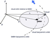Fig. 2. Motion of a cloud in an elliptical disc-like BLR around an SMBH in the barycentric coordinate frame. The blue arrow denotes the direction of the SMBH motion around the barycenter of the SMBBH system.

For notation simplicity, from now on we drop the iterative indexes i and j. To provide a more comprehensive practical illustration of our SMBBH geometrical model set-up, we applied it to the coplanar case of binary SMBHs whose elliptical disc-like BLRs are aligned with the binary common orbital plane. Each disc-like BLR is defined by the inner and outer radius, and an SMBH is located in its focus. The material in the discs rotates around the SMBH on the elliptical orbits with Keplerian rotation velocity (see Fig. 1b). The SMBH masses are M₁ = 10⁸ M_⊙ and M₂ = 0.5 × 10⁸ M_⊙. Their orbital eccentricities are 0.5 and the semimajor axis of the relative orbit is not larger than 30 ld. The inner and outer edges for the smaller and larger BLR are (4, 10) and (7, 15) ld, respectively. The eccentricities of the cloud orbits are 0.5.

In addition to a coplanar SMBBH, we also consider a non-coplanar case, when the SMBH orbits are mutually inclined. Such cases are well known in the multiple star population (see e.g. Schaefer et al. 2016). In hierarchical formation scenarios, if binary SMBH do not coalesce before the merger with a third galaxy, the formation of a triple SMBH system is possible. Most of such systems could be long-lived (∼10⁹ year) (see Amaro-Seoane et al. 2010, and references therein). However, we assumed a simple scenario, where mutually inclined SMBH orbits arise due to perturbation during a close encounter with some unseen massive object (such as an SMBH). This perturber has a much longer orbital period than the two components in a subparsec binary. The third object would be more distant and far away from the gravitational sphere of influence of SMBHs. Thus, we can omit a long-period perturber from consideration. This seems not an unrealistic assumption because there is an observed triple system of supermassive black holes, SDSS J150243.09+111557.3, at redshift z = 0.39, in which the closest pair is separated by ∼140 pc and the third active nucleus is at 7.4 kpc (Deane et al. 2015). In this case, the third SMBH is very far away from the gravitational influence of the tight pair because the gravitational sphere of influence of a black hole with masses of 10⁶ M_⊙ (Sagitarius A) is about 3 to 5 pc (Alexander 2011) and 10⁹ M_⊙ is about 100 pc (Deane et al. 2015). In this case, the reference plane is the orbital plane of one SMBH in the binary system and the frame of origin is set to the barycenter of the binary.

2.2. Kinematics of the disc-like BLR model

Now we derive the velocity of a cloud in the barycentric frame BXYZ (see Fig. 2). Here we list the formulas only for a cloud in a disc-like BLR of the more massive SMBH, and the derivation for less massive SMBH is similar. For the purpose of derivation, we rearrange Eq. (7) so that the vector of the relative position of a cloud [𝜚]_B in barycentric frame is given as

$$\begin{array}{c}\hfill \begin{array}{cc}& {[\mathit{\varrho }]}_{\mathrm{B}}={\mathit{r}}_{\mathrm{c}}-{\mathit{r}}_{\mathrm{b}},\hfill \end{array}\end{array}$$(9)

where r_b and r_c are barycentric positions of the SMBH and the cloud, respectively.

Simply from the transport theorem, we have that the barycentric velocity of a cloud is given by

$$\begin{array}{c}\hfill \begin{array}{cc}& {[\dot{\mathit{\varrho }}]}_{\mathrm{B}}={\dot{\mathit{\varrho }}}_{\bullet }+{\mathit{\omega }}_{\bullet /\mathrm{B}}\times {\mathit{\varrho }}_{\bullet },\hfill \end{array}\end{array}$$(10)

where ${\dot{\mathit{\varrho }}}_{\bullet }$ is the velocity vector of the cloud relative to the SMBH in the comoving frame of the SMBH (see Appendix C), and ω_•/B is equivalent to the angular velocity vector of the SMBH at each instant, which can be calculated from the known SMBH orbital angular momentum:

$$\begin{array}{c}\hfill {\mathit{\omega }}_{\bullet /\mathrm{B}}=\frac{{\mathit{r}}_{\mathrm{b}}\times {\dot{\mathit{r}}}_{\mathrm{b}}}{{\mathit{r}}_{\mathrm{b}}·{\mathit{r}}_{\mathrm{b}}}·\end{array}$$(11)

We note that ω_•/B can also be calculated using the barycentric orbital elements of the SMBH (see Eq. (C.4)). We can rephrase Eq. (11) in our set-up:

$$\begin{array}{c}\hfill \mathit{V}={\mathit{V}}_{\bullet }+{\mathit{\omega }}_{\bullet /\mathrm{B}}\times {\mathit{\varrho }}_{\bullet },\end{array}$$(12)

where ${\mathit{V}}_{\bullet }={\dot{\mathit{\varrho }}}_{\bullet }$. The relative state vectors (𝜚_• and V_•) of the cloud are given by Eqs. (C.25) and (C.26), respectively.

Having in mind Eq. (9), the time delay τ of each cloud is obtained as

$$\begin{array}{c}\hfill \tau =\frac{{|[\mathit{\varrho }]}_{\mathrm{B}}|+{\mathit{n}}_{\mathrm{obs}}·{[\mathit{\varrho }]}_{\mathrm{B}}}{c},\end{array}$$(13)

where |[𝜚]_B| is the norm of the relative position vector of a cloud in the barycentric frame and n_obs = (0, − sin i₀, − cos i₀) is the barycentric vector of the observer’s line of sight defined by the angle i₀. The relative barycentric position of the cloud can be obtained by transforming its relative position in the local comoving frame given by Eq. (C.27).

The velocity of the cloud (see Eq. (12)) projected onto the direction n_obs is

$$\begin{array}{c}\hfill V_z=\mathit{V}·{\mathit{n}}_{\mathrm{obs}}.\end{array}$$(14)

Expansions of equations for the projections of 𝜚 and velocity V_z are given in Appendix C.

2.3. Simple and composite transfer function

In the simple linear theory, the broad emission-line radial velocity V_z (given by Eq. (14)) and time-dependent response ℒ(V_z, t) is a convolution of prior time-delayed continuum variations 𝒞(t − τ) with a transfer function Ψ(V_z, τ) such that (Blandford & McKee 1982)

$$\begin{array}{c}\hfill \mathcal{L}(V_z,\tau )={\displaystyle {\int }_{-\infty }^{+\infty }}\mathcal{C}(t-\tau )\mathrm{\Psi }(V_z,\tau )\mathrm{d}\tau .\end{array}$$(15)

The transfer function is a projection of 6D (three spatial and three kinematical) phase space distribution into 2D phase space (defined by the radial velocity V_z and the time lag τ). The contribution of a particular cloud in a single BLR to the overall response depends on three parameters: its distance from the continuum source (setting the time delay of its response), its radial velocity (i.e. the velocity at which its response is observed), and the emissivity (the parameter describing the efficiency of the cloud in reprocessing the continuum into line photons in steady state). Based on the above discussion, we can predict the response of an emission line to continuum variations for any physical description of the BLR and probe the modelled transfer functions by comparing them to those that are inferred from observations. We aim here to predict these observational reverberation signatures for an elliptical disc model of the BLR of an SMBBH on elliptical orbits.

Thus the transfer function for a single elliptical disc can be written as follows:

$$\begin{array}{c}\hfill \mathrm{\Psi }(v,\tau )={\displaystyle \int ϵ(\varrho )}\delta (v-\mathit{V}{\mathit{n}}_{\mathrm{obs}})\delta (\mathit{ct}-(|\mathit{\varrho }|-\mathit{\varrho }·{\mathit{n}}_{\mathrm{obs}}))\mathrm{d}\mathit{\varrho }\mathrm{d}\mathit{V},\end{array}$$(16)

where ϵ(𝜚) is the (assumed isotropic) responding volume emissivity of the emission region as a function of position, and 𝜚, V are the barycentric state vectors of a cloud, but for clarity, the subscript B is omitted. We adopted the emissivity law ϵ(𝜚) = ϵ₀𝜚^−q (see Eracleous et al. 1995, and references therein) for calculating the 2DTF, where 𝜚 is the polar form of the trajectory of the cloud determined for a given time span starting from the solution of the Kepler equation. Because the trajectory is an ellipse, it implies that emissivity varies both with radial distance and the given true or eccentric anomaly and pericenter position of the cloud. The parameter q can take different values (see e.g. Eracleous et al. 1995; Popović et al. 2004; Afanasiev et al. 2019). Here we used q = 2.5 (Eracleous et al. 1995), which is expected in the case of moderate elongated annuli (e <  ∼0.55).

Because the orbital plane of a cloud is defined by inclination (i) and longitude of the ascending node (Ω), the transfer function of the elliptical disc can be given as follows:

$$\begin{array}{c}\hfill \mathrm{\Psi }(v,\tau )={ϵ}_0{\displaystyle {\int }_{R_{\mathrm{i}n}}^{R_{\mathrm{out}}}}{\varrho }^{-q}\mathrm{d}\varrho {\displaystyle {\int }_0^{2\pi }}\mathrm{d}\mathrm{\Omega }{\displaystyle {\int }_{-i_{\min }}^{i_{\max }}}sini\mathrm{d}i{\displaystyle {\int }_0^{2\pi }}\delta (X_1)\delta (X_2)\mathrm{d}E,\end{array}$$(17)

where X₁ = v − V_z, X₂ = ct − cτ, and E is the eccentric anomaly of the cloud on its orbital plane. Limits of integration i_min, i_max indicate the range of the orbit inclination of the cloud in a disc-like BLR, so that Θ = |i_max − i_min|.

Based on prescription from Paper I, the composite transfer function for an SMBBH system is obtained by calculating Ψ₁(v, τ) and Ψ₂(v, τ) for each BLR and coupling them as follows:

$$\begin{array}{c}\hfill \mathrm{\Psi }{(v,\tau )}_{\mathrm{coupled}}=\frac{{\mathrm{\Psi }}_1(v,\tau )}{1+{\mathrm{\Gamma }}_0}+\frac{{\mathrm{\Psi }}_2(v,\tau )}{1+{\mathrm{\Gamma }}_0^{-1}},\end{array}$$(18)

where Γ₀ is the coupling factor that is obtained by normalisation of the continuum variation of one of the SMBHs with the continuum of the other SMBH. Here we used the constant Γ₀ ∼ 1 as the simplest case when the binary black holes have the same properties as the continuum variations.

3. Results and discussion: Reverberation signatures of elliptical BLR model

The aim of this study is the differentiation of elliptical disc-like BLR models on the basis of 2DTF maps, therefore we calculated these maps for various adopted orbital configurations of the clouds and binary components. The time-averaged line profiles are also calculated and compared to those observed and inferred from disc-wind models.

For the initial conditions, we considered an SMBH binary with the same parameters as given in Paper I. The masses of the components are M₁ = 1 × 10⁸ M_⊙ and M₂ = 0.5 × 10⁸ M_⊙. We let the pericenters of the cloud orbits be uniformly distributed for the BLR around the primary (R_in, R_out)_c1 = (7, 15) ld and secondary component (R_in, R_out)_c2 = (4, 10) ld (see Eq. (8)). We generated 100 cloud orbits with a resolution of 1000 points each within the range of the given inner and outer boundaries of the disc-like BLRs. The inclination range for the cloud trajectories in the two disc-like BLR are Θ = 5^°. This assumption is in agreement with the hypothesis that a near-coplanar accretion disc and BLR could be expected because in gas-rich mergers, the evolution of the SMBBHs is due to interaction with the surrounding gas, so that the accretion onto the black holes align their spins with the angular momentum of the binary (Bogdanović et al. 2007). Our elliptical BLR models and binary geometry should be reduced to circular models when the eccentricity and the orbital orientation parameters are set to zero. Thus, the parameters presented in Paper I were used as a consistency check for our model. In this set-up, each mini-disc is illuminated by the continuum source at its own centre and not by the continuum source in the other disc.

In particular we considered models (i) with non-randomised orbital elements of clouds and (ii) with randomised eccentricities and/or an orbital orientation of the clouds. Specifically, for type (ii) simulations, we assumed that at the beginning, the clouds have random eccentricities and/or angles of orbital orientation. While eccentricities (and/or angles of orbital orientation) of clouds were chosen at random, their semimajor axes and inclinations were kept at their values as in the non- randomised case, thus ensuring non-intersecting orbital planes. In addition, clouds are considered to be dimensionless points whose motion has been followed on timescales of decades. We note here that our type (ii) model represents an idealised case where no cloud collision is taken into account. However, randomised cloud motion can be more complex than we have assumed in this work, and collisions between clouds could be present. Firstly, in a real situation the size of the clouds cannot be taken to be arbitrarily small. The BLR covering factor (i.e. the fraction of the sky that is covered by BLR clouds, as seen by the central source) is proportional to the space density of clouds (Mathews & Capriotti 1985). On the other hand, the averaged BLR covering factor is determined by estimating the fraction of ionising continuum photons that are absorbed by BLR clouds and reprocessed into broad emission lines, and it is constrained to be of ∼10% (using the equivalent widths of the broad emission lines, see e.g. Peterson 2006). Combining these two facts means that clouds on randomised orbits collide in about one orbital period (Mathews & Capriotti 1985). As a result, the system of clouds (or fluid elements) cannot remain on elliptical orbits for more than a few dynamical times, and it will settle down in a different configuration where the orbits are circular. When the elliptical orbits are to survive, they must therefore not cross. Second, as suggested by Mathews & Capriotti (1985) collisions may be reduced if the clouds resemble the motion of school of fish on a nearly circular orbit. Having this in mind, our model imputes a certain order in the cloud motion by constraints on their semimajor axes and inclinations, which can reduce the collision rates. For example, based on a geometrical approach (Courvoisier et al. 1996; Courvoisier & Türler 2005), we can roughly estimate that the collision rate of clouds is not so high (of about some hundred collisions per year for 10¹⁰ clouds at a distance of ∼10 ld from the SMBH), and probably that a small fraction of clouds on randomised orbits (at the beginning of our simulations) may collide during one orbital period, and after this, the emitted clouds follow orbits with a low probability of colliding. Otherwise, if the semimajor axes and inclinations could be random as well, the probability would be higher of crossing (intersecting) orbits, and collisions between clouds would be inevitable. In any case, the cloud collisions during randomised motion and implications on orbital stability will be considered in some further work, however.

A first glance reveals that the resulting response functions (for single and binary systems) are complex and differ substantially from those estimated by spherical disc-like BLR models in single SMBH and those in circular binaries. The geometry and kinematics of the elliptical BLR models determine the appearance of these maps. In the following subsections, we present a detailed description and discussion of the inferred 2DTF of a single SMBH, a binary SMBH system, and time-averaged line profiles for each of the given maps.

3.1. Simple 2DTF

The 2DTF maps of a single elliptical BLR that we presented in Fig. 3 have previously not been discussed, to our knowledge. Each map consists of two parts, a central region (2DTF core) and low flat wings on either side. A closer look reveals important nuances, however.

Fig. 3. 2DTF maps obtained for different geometries of a single disc-like BLR. The panels show signatures of (a) circular BLR as obtained using the parameters from Paper I (see text). Compare this with Fig. 2 in Paper I. b: elliptical BLR with clouds orbital parameters e = 0.5, Ω = 100°, and ω = 110°. c: orbital configurations of the clouds as given in (b), but with Ω = 0°; (d) the same orbital parameters as given in (b), but with ω = 0°; (e) the same as panel b, but the angles of the orbital orientation of clouds are random; (f) all three orbital parameters are random; (g) the orbital eccentricities of the clouds are random, but the orientation is the same as in panel b; (h) the orbital eccentricities of the clouds are random, but Ω = 10° and ω = 10°. We did not consider the stability of the elliptical orbits in the randomised motion.

Panel a shows the 2DTF that was obtained from our model using parameters for a single circular BLR (Ω = ω = 0°, and e = 0) as given in Paper I (see their Fig. 2a). The effects of eccentricity and orientation of the cloud elliptical orbits are illustrated in panels b−h. The shape of the maps is clearly asymmetric, where the well-known bell-like structure of the circular case is deformed. The orientation of the trajectories of the clouds visibly change the orientation of the map cores. It is interesting that both the longitude of ascending node and the angle of periastron are important for the map orientation. The effects of randomisation of eccentricities and orientation of orbits are shown in panels e−h (as we discussed above, in our model of randomised motion we did not consider the cloud collisions, which should be taken into account, and we postpone this consideration to a future study). The filaments of the 2DTF displayed a more chaotic appearance when the orbital orientations of clouds were randomised (e) in comparison with the regular and robust maps when only orbital eccentricities are random (g, h). The elongation of the red and blue wings depends on the angle of the pericenter. The red wing is more prominent when the angle of the pericenter increases and vice versa. The same holds when we consider that only eccentricities are random. Additionally, there is asymmetry in the monotonic appearance of the left and right sides of the 2DTF core. As shown in panels b, c, d, and g, the slopes of the left wings are steeper then the right ones, and this is controlled by the orbital orientation angles. For example, less steeply sloping gradients of the left wings occur when both orientation angles have low values (see panel h). The asymmetric 2DTF inferred from asymmetric models for the Seyfert 1 galaxy Mrk 50 (Pancoast et al. 2012) is similar to the map in panel h.

3.2. Composite 2DTF

Novel 2DTF maps of an elliptical binary system with elliptical disc-like BLRs are shown in Figs. 4–6. Each row of panels displays the 2DTF maps that correspond to the barycentric orbital configuration of the SMBH binary system given in the insets.

Fig. 4. 2DTF maps obtained for different geometries of a binary system with disc-like BLRs. The insets present the orbital phase of the binary system corresponding to the map. The direction of motion of the binary SMBH is anticlockwise. Panels a–c: coplanar circular case obtained using the parameters from Paper I (see their Fig. 2a); panels d–f: same as panels a–c, but the inclination of the smaller SMBH orbit is 30°; panels g–i: coplanar elliptical binary system with e = 0.5, Ω1 = Ω2 = 0°, ω1 = 0, and ω2 = 180°, and orbital parameters of the clouds of ec1 = ec2 = 0.5, Ωc1 = Ωc2 = 100°, ωc1 = 0°, and ωc2 = 180°; and panels j–l: same orbital parameters for the binary system as in panels g–i, but the orbital parameters of the clouds are ec1 = ec2 = 0.5, Ωc1 = Ωc2 =100°, and ωc1 = 110°, ωc2 = 290°.

Fig. 5. Same as Fig. 4. Panels a–c: coplanar elliptical binary system with e = 0.5, Ω1 = Ω2 = 0°, ω1 = 0, ω2 = 180°, clouds orbits in both BLRs have random eccentricities and Ωc1 = Ωc2 = 100°, ωc1 = 110°, ωc2 = 290°; panels d–f show that the plane of the more massive SMBH orbit is inclined by 30°, clouds in both disc-like BLR have an orientation ωc1 = 50°, ωc2 = 230°, and the remaining orbital parameters are the same as in panels a–c and g–i, except that the orbital eccentricities of the clouds are ec1 = 0.5 and ec2 = 0.1 and their orientations are randomised, all other orbital parameters are the same as in panels a–c; in panels j–l, the binary orbital configuration is the same as for panels d–f, but the orbital parameters of the clouds are random in both BLRs. (The stability of elliptical orbits is not considered.)

Fig. 6. Same as Fig. 4, but 10% of the clouds orbits are visible. From left to right: columns show orbital segments (kTcij/10, (k + 1)Tcij/10) for k ∈ {0, 4, 9} defined by the orbital period Tcij of the clouds. From the top down, panels a–c: elliptical binary system in which the orbital plane of the more massive SMBH is inclined by 30°, e = 0.5, Ω1 = Ω2 = 0°, ω1 = 0, and ω2 = 180°, and both discs are circular; panels d–f: same orbital configuration of the binary system as panels a–c, but their disc-like BLRs parameters are ec1 = ec2 = 0.5, Ωc1 = Ωc2 = 100°,ωc1 = 110°, and ωc2 = 290°; and panels g–i: same configuration of the binary system as panels a–c, and the orbital configurations of the BLR clouds are the same as in panels d–f, except that their eccentricities are random. The stability of the elliptical orbits in randomised motion is not considered.

The typical 2DTF maps of clouds with specific orbital parameters are shown in Fig. 4. The first row presents the maps for a circular SMBH system with circular disc-like BLRs as given in Paper I, in order to check the consistency of our binary SMBH model.

The second row depicts a non-coplanar SMBH system with circular BLRs with the same orbital parameters as above, but the orbital plane of the smaller SMBH is inclined by 30°. The orbital inclination of the SMBH shrinks the size and the shape of the 2DTF core of the smaller SMBH, which is evident in comparison with the previous case. Although they appear distinctive, the nuances between a coplanar and a non-coplanar circular binary would be difficult to discern without highly reliable reverberation mapping observations.

The third and forth row emphasize the effects of eccentricity and orientation angles of the orbits of the clouds and the coplanar SMBH. The maps in the third row suggest a significant degeneration of the bell shape when the argument of pericenter of the cloud is 180°. This means that the argument of pericenter of the cloud lies on the line of nodes and thus within the vicinity of the binary reference plane.

The effects of the inclined orbit of the larger SMBH in the binary system are shown in Fig. 5. For comparison, Figs. 5a–c shows the orbits of the coplanar elliptical binary SMBH. The hollow bell-shape of the more massive component caused by its inclined orbit is shown in the second row. The third and forth row show the effects of different combinations of randomised orbital cloud parameters (we did not consider the stability of elliptical orbits in the randomised motion). These maps illustrate a topology that is complex, as expected from similar maps in Fig. 3.

However, the orbital period of the binary might be too long to be easily observed (Begelman et al. 1980). Thus observations might cover only some portion of the full range of the period of the clouds and the binary motion. For these reasons, we analysed the case when clouds are observed for just 10% of their orbits, see Fig. 6. For example, the cloud takes about ten years to complete one orbit around the SMBH, but the monitoring campaign lasts just one year. Thus, orbital arcs of about one year in both BLRs would be covered by observations. The orbital arc starts at kT_cij/10 and ends at (k + 1)T_cij/10 for k ∈ {0, 4, 9}, defined by the orbital period T_cij of the cloud.

The insets present the orbital configuration of an SMBH system at the instances of the right edge of the orbital arcs of the cloud ((k+1)T_cij/10). The first row of panels show maps for elliptical SMBH orbits e = 0.5, while the orbital plane of the more massive SMBH is inclined by 30°, but both disc-like BLRs are circular. The remaining panels show maps for an elliptical SMBH with elliptical disc-like BLRs, but the third row contains the effects of random eccentricities of cloud trajectories in both discs (stability of elliptical orbits is not considered). When the orbital portion of each BLR cloud is observed for only one year, the orbit has a different structure. More compact structures are obtained in an orbital range of the clouds of (0, T_cij/10), and stripe-like structures are observed for (4T_cij/10, T_cij/2) and (9T_cij/10, T_cij). The circular (Fig. 6a) and elliptic (Figs. 6d and g) compact structures differ among themselves. The circular case (Figs. 6b and c) is similar to the simulated 49-day-long monitoring of the single circular BLR case in Horne et al. (2004, see their Fig. 3b). The randomisation of the eccentricity of the cloud trajectories deforms the stripe-like structures strikingly.

All 2DTFs presented here are strongly asymmetric with respect to the zero value of the radial velocity. In general, this means that either the blue or the red wing responds most rapidly.

3.3. Time-averaged spectral lines

Figures 7–10 display a series of velocity profiles obtained by integrating Ψ(v, τ) over the time delay (Blandford & McKee 1982),

$$\begin{array}{c}\hfill \mathrm{\Psi }(v)={\displaystyle {\int }_0^{{\tau }_{\max }}}\mathrm{\Psi }(v,\tau )\mathrm{d}\tau ,\end{array}$$(19)

where Ψ(v, τ) ≥ 0 for τ_max ∈ (0, ∞). It is a tim- averaged line profile that is the convolution of Ψ(v, τ) with a time-averaged continuum light curve because we do not have measured continuum variations (see Eq. (15)). Thus, the line profiles viewed here are time-averaged representatives of the emission line shapes that are expected for our models presented in Figs. 3–6.

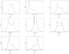Fig. 7. Spectrum corresponding to theoretical 2DTF maps obtained for different geometries of a single BLR in Fig. 3.

Fig. 8. Spectrum corresponding to theoretical 2DTF maps obtained for different geometries of the binary disc-like BLRs given in Fig. 4.

Fig. 9. Spectrum corresponding to theoretical 2DTF maps obtained for different geometries of the binary disc-like BLRs given in Fig. 5.

Fig. 10. Spectrum corresponding to theoretical 2DTF maps obtained for different geometries of portions of cloud orbits in the binary system given in Fig. 6.

The 1D projections of 2DTF of single BLR models (see Fig. 3) are shown in Fig. 7. The width and appearance of the spectral line is sensitive to the orientation of the cloud orbits. For fixed eccentricities and large Ω, increasing ω clearly broadens and blurs the typical double-peaked line profile of a Keplerian thin disc until one dominant horn is formed while the other peak is weakened. Simultaneously increasing either Ω or ω and reducing to zero the other orientation angle leads to double-peak profiles. Randomisation of eccentricities and/or orientation of clouds does not affect the appearance of the spectra significantly (stability of elliptical orbits is not considered).

The most interesting feature for these spectral line shapes is the asymmetrical double peak (with one peak more prominent than other). The features in Figs. 7c and g are detected in the spectra of PKS 1739+184 (PKS 1739+18C) observed by Lewis et al. (2010, see their Fig. 8). The feature from Fig. 7b is detected in spectra of Pictor A that was also observed by Lewis et al. (2010, see their Fig. 19 right column of panels). Interestingly, Eracleous et al. (2012, see their Fig. 2) found a similar shape of Hα and Hβ emission lines on SDSS J001224.02−102226.2 in their systematic search for close SMBBHs and rapidly recoiling black holes. Moreover, the features shown in Fig. 7h are very similar in appearance to the emission-line profiles of the disc-wind model present by Nguyen et al. (2019, compare to their Fig. 4 panel 5a), the Hubble space telescope observations of the Hα line of NGC 3147 (Bianchi et al. 2019, see their Fig. 2), and the Hβ emission line on SDSS J021259.60−003029.5 (Eracleous et al. 2012, see their Fig. 2). A similar feature is observed in the changing look NGC 3516 (De Rosa et al. 2018, see their Fig. 4). This example underlines that caution must be taken in interpreting disc-wind models that are solely inferred from spectral line shapes in the absence of detailed kinematic and 2DTF modelling.

Next, we present 1D dynamical models of emission lines obtained from 2DTF of the binary SMBH presented in Fig. 4. The plots in Fig. 8 reveal the primary effect of the phase of the SMBBH system: a prominent increase in flux at the line center. Profiles in the initial and the last phase of the coplanar circular binary system (see Figs. 8a and c) are broader than those obtained from its non-coplanar version (see Figs. 8d and f). Their orientation also depends on the phase. In the middle of the orbital period, the only difference is at the top of profile. In the case of the elliptical binary system, the emission line shapes depend on the orbital phase of the binary, but a small orientation angle of pericenter of the cloud orbits ω almost flattens the top of emission lines (see Figs. 8g–i). Conversely, higher values of ω tend to broaden the line shape in the initial orbital phase (Fig. 8j), and prominent core with double peaks in the middle (Fig. 8k) and final orbital phase (Fig. 8l). The wings are also asymmetric: the right wings are stronger because both SMBHs contribute to the system.

The effects of randomisation of eccentricities and/or orientation angles of the cloud orbit on the emission line shapes are shown in Fig. 9 (we did not consider the stability of the elliptical orbits). They were obtained from 2DTF maps presented in Fig. 5. The first row (Figs. 9a–c) shows emission lines obtained for the coplanar elliptical SMBBH system and cloud orbits with random eccentricities and higher values of ω (than in the case of Figs. 8g–i). The contribution of both SMBHs is clearly visible in the middle and final portion of orbital phase. Increasing the inclination of the elliptical orbit of the more massive SMBH and decreasing the angle of pericenter of the cloud orbits that have random eccentricities blurs the contribution of the emission of the less massive SMBH (see Figs. 9d–f). However, in the same non-coplanar settings of the SMBBH system, if we randomise the orientations of the clouds in both BLRs, but fix the eccentricities of the clouds of the more massive SMBH to a higher value (0.5) than the value of the less massive SMBH (0.1), the contribution of the less massive component is almost diminished and only a hint of its presence is visible as an asymmetry in the line profiles. On the other hand, a randomisation of the eccentricities and orientations of the clouds in both BLRs of the non-coplanar case terminates the contribution of the smaller SMBH around the middle (see Fig. 9k) and end of orbital phase (see Fig. 9l). A weak impression of the companion is visible at the beginning of the orbital period (see Fig. 9j).

The most interesting feature in Figs. 8a, c, d, f and 9b–f is an intermediate peak. This has been observed in the spectral lines of a few objects: 3C 390.3 by Popović et al. (2011, see their Fig. 1), Popović et al. (2014, see their Fig. 3), NGC 4151 (Shapovalova et al. 2008, see their Fig. 6), and E1821+643 (Shapovalova et al. 2016, see their Fig. 15). Additionally, the features shown in Figs. 9e–f and h–i are detected in the spectra of NGC 5548 (Peterson 1987, see their Fig. 3). Features in panels k–l are detected in the spectra of the spectral line in Mrk 668 (Liu et al. 2016, see their Fig. 1 lower spectrum).

Likewise, broad-line features such as shown in Figs. 8j and 9a are detected in BLR disc-wind models. The lines that form in the vicinity of the disc-wind base look broad and symmetric (see Yong et al. 2017). As already mentioned, disc-wind models and binary black holes can produce similar spectral line shapes, and a more thorough analysis is needed.

Next, we considered that only one year of the orbital period of the clouds of the non-coplanar elliptical binary SMBH system are observed in different SMBH orbital phases. As we show in Fig. 10, the emission line shapes vary remarkably. When the clouds are on circular trajectories in both BLRs, the right peak is more prominent at the beginning (see Fig. 10a) and middle of the orbital phase (see Fig. 9b). However, elliptical BLRs will produce a prominent left peak only in the middle and at the end of the orbital phase motion (see Figs. 10e and f). On the other hand, randomisation of the eccentricities in both BLRs broadens the emission lines (see Figs. 10g–i, but we did not consider the stability of elliptical orbits). The features in panel a are similar to the spectra of PKS 1346−112 (Eracleous & Halpern 2003, see their Fig. 1), and the Hβ emission line on SDSS J022014.57−072859.1 (Eracleous et al. 2012). The feature in panel b is also similar to artificial spectra in (Horne et al. 2004, see their Fig. 3b). The line shape in panel c looks like the Hβ emission line on SDSS J074007.28+410903.6 (Eracleous et al. 2012). The shape shown in panel f resembles the line features in Mrk 668 (Liu et al. 2016, see their Fig. 1 lower spectrum). The spectral line in panel e is a mirror image of the Hα line observed on SDSS J020011.53−093126.2 (Eracleous et al. 2012).

4. Conclusions

Here, by extending previous analysis in Paper I and II, we have presented a 3D geometrical model that self-consistently predicts the 2DTF signatures of an SMBBH system consisting of two binary SMBHs on elliptical orbits with elliptical disc-like BLRs. We considered a full set of orbital parameters of bot SMBHs in the system and clouds in both BLRs because our first goal was to understand the typical signatures of the BLR features in 2DTFs. We identified a number of characteristic features that might help in assessing the SMBBH system and in evaluating its parameters. Our main findings are listed below.

• 1.

  Simple and composite 2DTFs of elliptical disc-like BLRs have a deformed bell shape. The slope gradients and wing asymmetry of the deformed bells are predominantly controlled by the orbital orientation of the clouds. In particular, the 2DTF could serve as an advanced diagnostic tool to distinguish the BLR models on the basis of quantitative measurements.

• 2.

  Both simple and composite 2DTF exhibit further differentiation between randomly oriented or randomly elongated clouds trajectories and those where the orbital eccentricity or orientation of the cloud is fixed. The randomisation of the orbital parameters of the clouds tends to produce filaments in bells, which appeared to be more asymmetric and chaotic when the orbital orientation is random. As we discussed in Sect. 3, in our model of randomised motion we did not consider cloud collisions, which should be taken into account, and we postpone this consideration to a future study. An inclined SMBH orbit deforms the 2DTF bell size corresponding to its BLR.

• 3.

  In particular, we found a simple 2DTF (inferred from a single SMBH model) that we calculated for small angles of orientation and random eccentricities of the clouds orbits, similar to that observed in Mrk 50. We did not consider the stability of elliptical orbits during randomised motion.

• 4.

  An overall degeneracy of the 2DTF maps is observed for the hypothetical case when the cloud orbit is observed for only one year. The presence of two discs is clear when the observations cover the first tenth of the orbital periods of the clouds. This means that the length of monitoring campaigns must be long enough to sample the full range of time lags, which can help to constrain the parameters of dynamical models.

• 5.

  The simulations show that an intermediate peak in the broad-line profiles such as that observed in NGC 4151, NGC 5548, and 3C 390.3 can indeed be reproduced by our elliptical binary model.

• 6.

  We found a remarkable coincidence between the line distortions produced for the disc-wind and elliptical BLR models. A good distinction between these BLR models would require long-term and quality-cadenced spectrophotometric monitoring.

Acknowledgments

We appreciate and thank an anonymous Referee for invaluable comments. This work is supported by the Ministry of Education, Science and Technological development of Republic Serbia through the Astrophysical Spectroscopy of Extragalactic Objects project number 176001, National Key R&D Program of China (grant 2016YFA0400701) and grants NSFC-11173023, -11133006, -11373024, -11233003, -11473002, and by CAS Key Research Program of Frontier Sciences, QYZDJ–SSW–SLH007. JMW is supported by National Key R&D Program of China through grant 2016YFA0400701, by NSFC through grants NSFC-11991050, -11873048.

References

Appendix A: Geometric description of orbits

Firstly, we introduce the general framework we used for any orbital motion description, which is standard astrometric notation (Fig. 1a). If the reference coordinate system XYZ with origin in object O is arbitrary chosen, let the object of mass M be in an elliptical orbit about object O moving in anticlockwise direction, so that its orbital position radius vector OM has a value r at time t. If a set of axes Oξ and Oη are taken in the plane of the orbit with Oξ along the major axis of the elliptical orbit towards the pericenter P and Oη, perpendicular to the major axis, then the coordinates of M relative to this set of axes are ξ and η given by

$$\begin{array}{c}\hfill \mathit{r}=\left\{\begin{array}{c}\xi \\ \eta \\ 0\end{array}\right\}=\left\{\begin{array}{c}rcosf\\ rsinf\\ 0\end{array}\right\},\end{array}$$(A.1)

and

$$\begin{array}{c}\hfill \mathit{v}=\left\{\begin{array}{c}\dot{\xi }\\ \dot{\eta }\\ 0\end{array}\right\}=\left\{\begin{array}{c}{\displaystyle \frac{-nasinf}{\sqrt{1-e^2}}}\\ {\displaystyle \frac{na(e+cosf)}{\sqrt{1-e^2}}}\\ 0\end{array}\right\},\end{array}$$(A.2)

where f = ∠POM is a true anomaly defined as the angle at the focus O between the direction of perihelion and the position radius vector OM of the body M, $r=\frac{p}{1+ecosf}$ is the norm of the position radius vector OM, a is the semimajor axis of the elliptical orbit, e is the eccentricity of the elliptical orbit that defines the amplitude of the oscillations in r at time t. Furthermore, T and n are the orbital period and the mean angular frequency (or the mean motion, defined as n = 2π/T) of object M. Because integrating the velocity in an elliptical orbit is difficult, a convenient method uses the concept of a reference circle centred on the centre of the elliptical orbit with a radius equal to the semimajor axis, so that the vectors of position and velocity are given as follows:

$$\begin{array}{c}\hfill \mathit{r}=\left\{\begin{array}{c}a(cosE-e)\\ a\sqrt{1-e^2}sinE\\ 0\end{array}\right\},\end{array}$$(A.3)

and

$$\begin{array}{c}\hfill \mathit{v}=\left\{\begin{array}{c}{\displaystyle \frac{-n{a}^2}{r}sinE}\\ {\displaystyle \frac{n{a}^2}{r}\sqrt{1-e^2}cosE}\\ 0\end{array}\right\},\end{array}$$(A.4)

where E is the eccentric anomaly defined in Appendix B, an angular variable that also represents the phase of the oscillation in r, and r = a(1 − e cos E) is the norm of the position radius vector at a given time. The point of closest approach (i.e. the orbital pericenter) of body M to O is at E = f = 0, so that E = f = π corresponds to the apocenter and p is the semilatus rectum of the elliptical orbit of object M.

The representation of the orbit of object M in 3D is also illustrated in Fig. 1a. The orbital plane intersects the reference plane of the coordinate system on a line called the line of nodes N′ON. If the direction in which the object moves on its orbit is anticlockwise, N is referred to as the ascending node. Then the longitude of the ascending node Ω is given by ∠XON measured in the reference plane from 0 to 2π. The inclination i is the angle between the reference and the orbital plane. The argument of pericenter ω = ∠NOP is the angle from the body’s ascending node to its pericenter P, measured in the direction of motion in the orbital plane.

The expression of the orbital position and velocity in 3D is found by transforming the state vector from the apsidal frame to 3D by applying

$$\begin{array}{cc}\hfill {\mathit{r}}^{″}& ={\mathbb{P}}^{\mathrm{T}}\mathit{r},\hfill \end{array}$$(A.5)

$$\begin{array}{cc}\hfill {\mathit{v}}^{″}& ={\mathbb{P}}^{\mathrm{T}}\mathit{v},\hfill \end{array}$$(A.6)

where in terms of inclination (i), argument of pericenter (ω) and angle of ascending node (Ω) of a given orbit,

$$\begin{array}{cc}& \mathbb{P}=\hfill \\ \hfill & \left\{\begin{array}{ccc}cos\mathrm{\Omega }cos\omega -sin\mathrm{\Omega }sin\omega cosi& sin\mathrm{\Omega }cos\omega +cos\mathrm{\Omega }sin\omega cosi& sin\omega sini\\ -cos\mathrm{\Omega }sin\omega -sin\mathrm{\Omega }cos\omega cosi& -sin\mathrm{\Omega }sin\omega +cos\mathrm{\Omega }cos\omega cosi& cos\omega sini\\ sin\mathrm{\Omega }sini& -cos\mathrm{\Omega }sini& cosi\end{array}\right\}.\hfill \\ \hfill \end{array}$$(A.7)

Because the direction cosine matrix ℙ consists of three rotations that are orthogonal, its inverse is just its transpose or ℙ^T. The orientation of the elliptic orbit in the coordinate system depends on the inclination i, the angle of the ascending node Ω, and the argument of pericenter ω. If the inclination is zero, the orbit is located in the X − Y plane. As the eccentricity increases, the pericenter will be in the +X direction. If the inclination is increased, the ellipse will be rotating around the X-axis, so that +Y is rotated toward +Z. An increase in Ω is the rotation of +X toward +Y. A variation of ω alters the orbit position only in the orbital plane.

A.1. Introducing time in the model

We note that state vectors are functions of the astrometric angles. The position and velocity of an SMBH and clouds in their orbital planes at a given time depend on their phases in orbits, which are defined by their true anomalies (e.g. Murray & Dermott 1999). In the circular orbit limit e → 0, the orbital phase is simply f = 2πΦ(t − t₀), where Φ is the Keplerian orbital frequency and t₀ is the pericenter passage (see Paper I). However, for eccentric orbits, the non-linear relative angular positions between two bodies in motion about their centre of mass is related to linearly advancing time through the Kepler equation. When the object passes through pericenter at t = t₀, and its orbital period is T, the dimensionless variable l = 2π(t − t₀)/T = n(t − t₀) is referred to as the mean anomaly, where n is the mean angular frequency (or mean motion), n = 2π/T. We numerically solved the transcendental Kepler equation for the eccentric anomaly E:

$$\begin{array}{c}\hfill l=E-esinE.\end{array}$$(A.8)

Furthermore, the true (f) and eccentric (E) anomaly are related by (see Appendix B, Eq. (B.11))

$$\begin{array}{c}\hfill tan\frac{f}{2}=\sqrt{\frac{1+e}{1-e}}tan\frac{E}{2},\end{array}$$(A.9)

where f establishes the temporal variation of the phase of the object on its orbit. Thus we can obtain the position and velocity of the object at any given time t. Clearly, the phase is related to the inverse of the tangent of the eccentric anomaly, and the latter is related in transcendental form as the Kepler equation to the mean motion n = 2π/T and thus to the frequency n = 2πΦ = 2π/T.

Knowing the average angular frequency and the eccentricity of the orbit of the object, we solved the transcendental Eq. (A.8) for E at a given time t, where l is calculated as l = 2π(t − t₀)/T. The eccentric anomaly was then substituted into Eq. (A.9) to give the phase f. After this, the eccentric anomaly was plugged into Eq. (A.4) to obtain the position and velocity at any point along the orbit. We assumed that time and phase are measured from the moment of passage through pericenter, then the constant t₀ can be set to zero.

A.2. Relative motion in the orbit

Taking into account the relative motion of the SMBH with respect to the barycenter, we derived the transformation of the vectors between the barycentric and the comoving frame attached to the SMBH. We assumed that the position of the more massive SMBH in the barycentric coordinate frame of the coplanar binary case is r_b1. The moving frame of reference has its origin at the SMBH and is orbiting the barycenter of the binary. The x-axis is directed along the outward radial r_b1 to the SMBH. Thus the unit vector $\widehat{\mathit{i}}$ along the moving axis is

$$\begin{array}{c}\hfill \widehat{\mathit{i}}=\frac{{\mathit{r}}_{\mathrm{b}1}}{r_{\mathrm{b}1}}·\end{array}$$(A.10)

The z-axis of the moving frame is normal to the orbital plane of the SMBH, lying in the direction of the angular momentum vector of the SMBH. Its unit vector is given by

$$\begin{array}{c}\hfill \widehat{\mathit{k}}=\frac{{\mathit{r}}_{\mathrm{b}1}\times {\mathit{v}}_{\mathrm{b}1}}{|{\mathit{r}}_{\mathrm{b}1}\times {\mathit{r}}_{\mathrm{b}1}|}·\end{array}$$(A.11)

The y-axis is perpendicular to both $\widehat{\mathit{i}}$ and $\widehat{\mathit{k}}$, with the unit vector completing the right triad of the moving frame, that is,

$$\begin{array}{c}\hfill \widehat{\mathit{j}}=\widehat{\mathit{k}}\times \widehat{\mathit{i}}.\end{array}$$(A.12)

The transformation of any vector s_B from the barycentric to the local SMBH moving frame is given by

$$\begin{array}{c}\hfill {\mathit{s}}_{\bullet }=\mathbb{Q}{\mathit{s}}_{\mathrm{B}},\end{array}$$(A.13)

where the matrix ℚ consists of rows of the unit vector coordinates defined above:

$$\begin{array}{c}\hfill \mathbb{Q}=\left\{\begin{array}{c}\widehat{\mathit{i}}\hfill \\ \widehat{\mathit{j}}\hfill \\ \widehat{\mathit{k}}\hfill \end{array}\right\},\end{array}$$(A.14)

and the inverse transformation from the local to the barycentric system is given by s_B = ℚ⁻¹s_•.

In the non-coplanar case the local reference plane of the inclined SMBH does not coincide with the general reference plane.

Appendix B: Relation between the eccentric and the true anomaly

The relation between the eccentric (E) and the true anomaly (f) defined in Eq. (A.9) is derived by following geometrical consideration. A circumcircle is described on AA′ as the diameter around the ellipse, as shown in Fig. B.1. PR is perpendicular to AA′ and intersects the circumcircle in Q, the angle QCA is the eccentric anomaly E, and it is related to the true anomaly f.

Fig. B.1. Scheme for deriving the relation between the true and mean anomaly. C is the common centre of the ellipse and the auxiliary circle. S is the focus of the ellipse. The semimajor and semiminor axes are CA = a and CB = b, respectively. The orbital postion of the object is P, its perpendicular projection on the semimiajor axis is R, and the intersection of PR and the auxiliary circle is Q. |SP|=r and CS = ae, where e is the eccentricity of ellipse. The angles ∠QCA and ∠PSA are the eccentric and the true anomaly, respectively. The radius of the auxiliary circle equals the orbital semimajor axis.

From the geometry, it is easy to see that

$$\begin{array}{cc}\hfill \mathrm{SR}& =\mathrm{CR}-\mathrm{CS}=acosE-ae,\hfill \end{array}$$(B.1)

$$\begin{array}{cc}\hfill \mathrm{SR}& =rcosf,\hfill \end{array}$$(B.2)

and hence

$$\begin{array}{c}\hfill rcosf=a(cosE-e).\end{array}$$(B.3)

According to the property of the ellipses and circumscribed circles,

$$\begin{array}{cc}& \frac{\mathrm{PR}}{\mathrm{QR}}=\frac{b}{a},\hfill \end{array}$$(B.4)

$$\begin{array}{cc}& rsinf=bsinE=a\sqrt{1-e^2}sinE.\hfill \end{array}$$(B.5)

Squaring and summing Eqs. (B.3) and (B.5), we obtain

$$\begin{array}{c}\hfill r=a(1-ecosE).\end{array}$$(B.6)

Now, using trigonometry,

$$\begin{array}{c}\hfill rcosf=r({cos}^2\frac{f}{2}-{sin}^2\frac{f}{2})=r(1-2{sin}^2\frac{f}{2}),\end{array}$$(B.7)

so that

$$\begin{array}{c}\hfill 2r{sin}^2\frac{f}{2}=r(1-cosf).\end{array}$$(B.8)

Using Eqs. (B.3) and (B.6), we obtain

$$\begin{array}{c}\hfill 2r{sin}^2\frac{f}{2}=a(1+e)(1-cosE).\end{array}$$(B.9)

With similar reasoning, it is easy to obtain

$$\begin{array}{c}\hfill 2r{cos}^2\frac{f}{2}=a(1-e)(1+cosE).\end{array}$$(B.10)

Dividing Eq. (B.9) by Eq. (B.10), we finally obtain the relation between the eccentric and the true anomaly,

$$\begin{array}{c}\hfill tan\frac{f}{2}=\sqrt{\frac{1+e}{1-e}}tan\frac{E}{2}·\end{array}$$(B.11)

The eccentric anomaly is an angular variable that represents the phase of the oscillation in radial position of a body on an elliptical orbit.

Appendix C: Expansions of vectorial equations for velocity-delay maps

Here we list expansions of the equations of the barycentric state vectors of M₁ (see Eq. (6)), the radial position of the jth cloud in its BLR with respect to the barycenter (see Eq. (7)), the barycentric velocity of the cloud (Eq. (10)), and the projection of the cloud barycentric vector of the relative position and velocity (see Eqs. (13) and (12)) on the observed line of sight ( n_obs = (0, − sin i₀, − cos i₀)). For practical reasons, the subscript 1 is omitted for SMBH orbital elements, and we use the short notations

$$\begin{array}{cc}& b=a\sqrt{1-e^2},\hfill \end{array}$$(C.1)

$$\begin{array}{cc}& r=a(1-ecosE),\hfill \end{array}$$(C.2)

$$\begin{array}{cc}& h=\sqrt{G\frac{M_1+M_2}{a_{\mathrm{B}}}}\frac{M_1{M}_2}{M_1+M_2}{b}_{\mathrm{B}},\hfill \end{array}$$(C.3)

$$\begin{array}{cc}& {\mathit{\omega }}_{\bullet /\mathrm{B}}=h\left\{\begin{array}{c}sin\mathrm{\Omega }sini\\ -cos\mathrm{\Omega }sini\\ cosi\end{array}\right\},\hfill \end{array}$$(C.4)

$$\begin{array}{cc}& n=\frac{2\pi }{T},\hfill \end{array}$$(C.5)

$$\begin{array}{cc}& w_{11}=cos\mathrm{\Omega }cos\omega -sin\mathrm{\Omega }sin\omega cosi,\hfill \end{array}$$(C.6)

$$\begin{array}{cc}& w_{12}=sin\mathrm{\Omega }cos\omega +cos\mathrm{\Omega }sin\omega cosi,\hfill \end{array}$$(C.7)

$$\begin{array}{cc}& w_{13}=sin\omega sini,\hfill \end{array}$$(C.8)

$$\begin{array}{cc}& w_{21}=-cos\mathrm{\Omega }sin\omega -sin\mathrm{\Omega }cos\omega cosi,\hfill \end{array}$$(C.9)

$$\begin{array}{cc}& w_{22}=-sin\mathrm{\Omega }sin\omega +cos\mathrm{\Omega }cos\omega cosi,\hfill \end{array}$$(C.10)

$$\begin{array}{cc}& w_{23}=cos\omega sini,\hfill \end{array}$$(C.11)

$$\begin{array}{cc}& {\mathbb{Q}}^{-1}=[q_{\mathit{ij}}],i,j=1,3,\hfill \end{array}$$(C.12)

where h in Eq. (C.3) is the norm of the total angular momentum of the barycentric system, which is written in terms of the semimajor a_B and semiminor b_B axis of the ellipse that is swept by the vector of the relative position of M₂ with respect to M₁ (see Bradt 2008). We note that in Eqs. (C.6)–(C.12) numbers 1 and 2 have descriptive meaning and are not the vector components of a certain SMBH. Their forms are invariant under coordinate system transformations. Likewise, we can introduce short notations for the parameters related to the cloud orbits in a moving frame,

$$\begin{array}{cc}& b_{\mathrm{c}}=a_{\mathrm{c}}\sqrt{1-e_{\mathrm{c}}^2},\hfill \end{array}$$(C.13)

$$\begin{array}{cc}& r_{\mathrm{c}}=a_{\mathrm{c}}(1-e_{\mathrm{c}}cos{E}_{\mathrm{c}}),\hfill \end{array}$$(C.14)

$$\begin{array}{cc}& n_{\mathrm{c}}=\frac{2\pi }{T_{\mathrm{c}}},\hfill \end{array}$$(C.15)

$$\begin{array}{cc}& w_{11}^{\mathrm{c}}=cos{\mathrm{\Omega }}_{c}cos{\omega }_c-sin{\mathrm{\Omega }}_{c}sin{\omega }_{c}cos{i}_c,\hfill \end{array}$$(C.16)

$$\begin{array}{cc}& w_{12}^c=sin{\mathrm{\Omega }}_{\mathrm{c}}cos{\omega }_{\mathrm{c}}+cos{\mathrm{\Omega }}_{\mathrm{c}}sin{\omega }_{\mathrm{c}}cos{i}_{\mathrm{c}},\hfill \end{array}$$(C.17)

$$\begin{array}{cc}& w_{13}^{\mathrm{c}}=sin{\omega }_{\mathrm{c}}sin{i}_{\mathrm{c}},\hfill \end{array}$$(C.18)

$$\begin{array}{cc}& w_{21}^{\mathrm{c}}=-cos{\mathrm{\Omega }}_{\mathrm{c}}sin{\omega }_{\mathrm{c}}-sin{\mathrm{\Omega }}_{\mathrm{c}}cos{\omega }_{\mathrm{c}}cos{i}_{\mathrm{c}},\hfill \end{array}$$(C.19)

$$\begin{array}{cc}& w_{22}^{\mathrm{c}}=-sin{\mathrm{\Omega }}_{\mathrm{c}}sin{\omega }_{\mathrm{c}}+cos{\mathrm{\Omega }}_{\mathrm{c}}cos{\omega }_{\mathrm{c}}cos{i}_{\mathrm{c}},\hfill \end{array}$$(C.20)

$$\begin{array}{cc}& w_{23}^{\mathrm{c}}=cos{\omega }_{\mathrm{c}}sin{i}_{\mathrm{c}},\hfill \end{array}$$(C.21)

$$\begin{array}{cc}& {\mathbb{Q}}^{-1}=[q_{\mathit{ij}}],i,j=1,3.\hfill \end{array}$$(C.22)

The transformation ℚ⁻¹ is an inverse of the transformation defined by Eq. (A.14), and allows us to transform the vector from the comoving to the barycentric frame. We note that Eqs. (C.6)–(C.12) and (C.16)–(C.22) could be reduced to a simpler form for Ω = 0 and Ω_c = 0.

For a given set of elements, the mean motion n and the time, the barycentric coordinates, and the velocity components of M₁ can be computed as follows:

$$\begin{array}{cc}\hfill {\mathit{r}}_{\mathrm{b}}& =r\frac{M_2}{M_1+M_2}\left\{\begin{array}{c}a{w}_{11}cosE+b{w}_{21}sinE-a{w}_{11}\hfill \\ a{w}_{12}cosE+b{w}_{22}sinE-ae{w}_{11}\hfill \\ a{w}_{13}cosE+b{w}_{23}sinE-ae{w}_{13}\hfill \end{array}\right\}\hfill \end{array}$$(C.23)

$$\begin{array}{cc}\hfill {\mathit{v}}_{\mathrm{b}}& =\frac{M_2}{M_1+M_2}\frac{\mathit{na}}{r}\left\{\begin{array}{c}b{w}_{21}cosE-a{w}_{11}sinE\hfill \\ b{w}_{22}cosE-a{w}_{12}sinE\hfill \\ b{w}_{23}cosE-a{w}_{13}sinE\hfill \end{array}\right\}.\hfill \end{array}$$(C.24)

Similarly, the vector of the cloud position and velocity in a 3D SMBH comoving frame is given as

$$\begin{array}{cc}\hfill {\mathit{\varrho }}_{\bullet }& =r_{\mathrm{c}}\left\{\begin{array}{c}{a}_{\mathrm{c}}{w}_{11}^{\mathrm{c}}cos{E}_{\mathrm{c}}+b_{\mathrm{c}}{w}_{21}^{\mathrm{c}}sin{E}_{\mathrm{c}}-a_{\mathrm{c}}{w}_{11}^{\mathrm{c}}\hfill \\ a_{\mathrm{c}}{w}_{12}^{\mathrm{c}}cos{E}_{\mathrm{c}}+b_{\mathrm{c}}{w}_{22}^{\mathrm{c}}sin{E}_{\mathrm{c}}-a_{\mathrm{c}}{e}_{\mathrm{c}}{w}_{12}^{\mathrm{c}}\hfill \\ a_{\mathrm{c}}{w}_{13}^{\mathrm{c}}cos{E}_{\mathrm{c}}+b_{\mathrm{c}}{w}_{23}^{\mathrm{c}}sin{E}_{\mathrm{c}}-a\mathrm{c}{e}_{\mathrm{c}}{w}_{13}^{\mathrm{c}}\hfill \end{array}\right\}\hfill \end{array}$$(C.25)

$$\begin{array}{cc}\hfill {\dot{\mathit{\varrho }}}_{\bullet }& =\frac{n_{\mathrm{c}}{a}_{\mathrm{c}}}{r_{\mathrm{c}}}\left\{\begin{array}{c}{b}_{\mathrm{c}}{w}_{21}^{\mathrm{c}}cos{E}_{\mathrm{c}}-a_{\mathrm{c}}{w}_{11}^{\mathrm{c}}sin{E}_{\mathrm{c}}\hfill \\ b_{\mathrm{c}}{w}_{22}^{\mathrm{c}}cos{E}_{\mathrm{c}}-a_{\mathrm{c}}{w}_{12}^{\mathrm{c}}sin{E}_{\mathrm{c}}\hfill \\ b_{\mathrm{c}}{w}_{23}^{\mathrm{c}}cos{E}_{\mathrm{c}}-a_{\mathrm{c}}{w}_{13}^{\mathrm{c}}sin{E}_{\mathrm{c}}\hfill \end{array}\right\}.\hfill \end{array}$$(C.26)

Thus the relative position of the cloud in the barycentric frame is calculated by the transformation ℚ⁻¹, which is the inverse of the transformation defined by Eq. (A.14) at each time instant:

$$\begin{array}{c}\hfill \begin{array}{cc}& {[\mathit{\varrho }]}_{\mathrm{B}}={\mathbb{Q}}^{-1}{[\mathit{\varrho }]}_{\bullet }.\hfill \end{array}\end{array}$$(C.27)

The characterisation of the motion of the SMBH coordinate frame is given by specifying the angular velocity vector of the SMBH. Because the SMBH coordinate frame is also a body frame of the SMBH, the angular velocity of the SMBH is also the angular velocity of the frame. The barycentric angular velocity of the SMBH is given by Eq. (C.3). The velocity of the cloud in the barycentric frame as time-derivative is calculated through the basic kinematic equation or transport theorem (see Eq. (10)). Thus, the elements of the projections of [𝜚]_B on the observer’s line of sight are given by

$$\begin{array}{cc}\hfill {[\mathit{\varrho }]}_{\mathrm{B}}·{\mathit{n}}_{\mathrm{obs}}=& -sin{i}_0(q_{21}{r}_{\mathrm{c}}(a_{\mathrm{c}}{w}_{11}^{\mathrm{c}}cos{E}_{\mathrm{c}}-a_{\mathrm{c}}{w}_{11}^{\mathrm{c}}+b_{\mathrm{c}}{w}_{21}^{\mathrm{c}}sin{E}_{\mathrm{c}})\hfill \\ \hfill & +q_{22}{r}_{\mathrm{c}}(-a_{\mathrm{c}}{e}_{\mathrm{c}}{w}_{12}^{\mathrm{c}}+a_{\mathrm{c}}{w}_{12}^{\mathrm{c}}cos{E}_{\mathrm{c}}+b_{\mathrm{c}}{w}_{22}^{\mathrm{c}}sin{E}_{\mathrm{c}})\hfill \\ \hfill & +q_{23}{r}_{\mathrm{c}}(-a_{\mathrm{c}}{e}_{\mathrm{c}}{w}_{13}^{\mathrm{c}}+a_{\mathrm{c}}{w}_{13}^{\mathrm{c}}cosE\_\mathrm{c}+b_{\mathrm{c}}{w}_{23}^{\mathrm{c}}sin{E}_{\mathrm{c}}))\hfill \\ \hfill & -cos{i}_0(q_{31}{r}_{\mathrm{c}}(a_{\mathrm{c}}{w}_{11}^{\mathrm{c}}cos{E}_{\mathrm{c}}-a_{\mathrm{c}}{w}_{11}^{\mathrm{c}}+b_{\mathrm{c}}{w}_{21}^{\mathrm{c}}sin{E}_{\mathrm{c}})\hfill \\ \hfill & +q_{32}{r}_{\mathrm{c}}(-a_{\mathrm{c}}{e}_{\mathrm{c}}{w}_{12}^{\mathrm{c}}+a_{\mathrm{c}}{w}_{12}^{\mathrm{c}}cos{E}_{\mathrm{c}}+b_{\mathrm{c}}{w}_{22}^{\mathrm{c}}sin{E}_{\mathrm{c}})\hfill \\ \hfill & +q_{33}{r}_{\mathrm{c}}(-a_{\mathrm{c}}{e}_{\mathrm{c}}{w}_{13}^{\mathrm{c}}+a_{\mathrm{c}}{w}_{13}^{\mathrm{c}}cos{E}_{\mathrm{c}}+b_{\mathrm{c}}{w}_{23}^{\mathrm{c}}sin{E}_{\mathrm{c}})).\hfill \end{array}$$(C.28)

Likewise, the elements of the projections V on the observer’s line of sight is obtained as follows:

$$\begin{array}{cc}\hfill V_z=& \mathit{V}·{\mathit{n}}_{\mathrm{obs}}=\frac{1}{r_{\mathrm{c}}}(-a_{\mathrm{c}}(cos{E}_{\mathrm{c}}{b}_{\mathrm{c}}{n}_{\mathrm{c}}(cos{i}_0{w}_{23}^{\mathrm{c}}+w_{22}^{\mathrm{c}}sin{i}_0)\hfill \\ \hfill & +h{r}_{\mathrm{c}}^2(cos{E}_{\mathrm{c}}{w}_{11}^{\mathrm{c}}(cos{i}_{0}cos\mathrm{\Omega }si+cosisin{i}_0)\hfill \\ \hfill & +(cos{E}_{\mathrm{c}}-e_{\mathrm{c}})sini(cos{i}_0{w}_{12}^{\mathrm{c}}-w_{13}^{\mathrm{c}}sin{i}_0)sin\mathrm{\Omega }))\hfill \\ \hfill & +(a_{\mathrm{c}}^2{n}_{\mathrm{c}}(cos{i}_0{w}_{13}^{\mathrm{c}}+w_{12}^{\mathrm{c}}sin{i}_0)sin{E}_{\mathrm{c}}\hfill \\ \hfill & +h{r}_{\mathrm{c}}^2(a{w}_{11}^{\mathrm{c}}(cos{i}_{0}cos\mathrm{\Omega }sini+cos{i}_{0}sin{i}_0)))\hfill \\ \hfill & -(b_{\mathrm{c}}{w}_{21}^{\mathrm{c}}(cos{i}_{0}cos\mathrm{\Omega }sini+cos{i}_{0}sin{i}_0)\hfill \\ \hfill & +b_{\mathrm{c}}sini(cos{i}_0{w}_{22}^{\mathrm{c}}-w_{23}^{\mathrm{c}}sin{i}_0)sin\mathrm{\Omega })sin{E}_{\mathrm{c}}).\hfill \end{array}$$(C.29)

All Figures

Fig. 1. Panel a: orbit of body M described with the standard astrometric set of orbital elements (a, e, i, ω, Ω, f), where POM = f is the true anomaly and L is the angular momentum vector of the motion of the body. The inertial OXYZ coordinate system can be chosen arbitrarily (see the detailed explanation in Appendix A). Panel b: realisation of the coplanar elliptical SMBBH system at the half orbital period calculated from our binary system model. M1 and M2 are the locations of the SMBHs in a binary system. Blue ellipses are the inner and outer boundaries of disc-like BLRs. The reference plane (BXY) is the plane of the relative orbit of M2 with respect to M1, and the origin of the coordinate system is the barycenter (B) of the system.

In the text

	Fig. 2. Motion of a cloud in an elliptical disc-like BLR around an SMBH in the barycentric coordinate frame. The blue arrow denotes the direction of the SMBH motion around the barycenter of the SMBBH system.
In the text

Fig. 3. 2DTF maps obtained for different geometries of a single disc-like BLR. The panels show signatures of (a) circular BLR as obtained using the parameters from Paper I (see text). Compare this with Fig. 2 in Paper I. b: elliptical BLR with clouds orbital parameters e = 0.5, Ω = 100°, and ω = 110°. c: orbital configurations of the clouds as given in (b), but with Ω = 0°; (d) the same orbital parameters as given in (b), but with ω = 0°; (e) the same as panel b, but the angles of the orbital orientation of clouds are random; (f) all three orbital parameters are random; (g) the orbital eccentricities of the clouds are random, but the orientation is the same as in panel b; (h) the orbital eccentricities of the clouds are random, but Ω = 10° and ω = 10°. We did not consider the stability of the elliptical orbits in the randomised motion.

In the text

Fig. 4. 2DTF maps obtained for different geometries of a binary system with disc-like BLRs. The insets present the orbital phase of the binary system corresponding to the map. The direction of motion of the binary SMBH is anticlockwise. Panels a–c: coplanar circular case obtained using the parameters from Paper I (see their Fig. 2a); panels d–f: same as panels a–c, but the inclination of the smaller SMBH orbit is 30°; panels g–i: coplanar elliptical binary system with e = 0.5, Ω1 = Ω2 = 0°, ω1 = 0, and ω2 = 180°, and orbital parameters of the clouds of ec1 = ec2 = 0.5, Ωc1 = Ωc2 = 100°, ωc1 = 0°, and ωc2 = 180°; and panels j–l: same orbital parameters for the binary system as in panels g–i, but the orbital parameters of the clouds are ec1 = ec2 = 0.5, Ωc1 = Ωc2 =100°, and ωc1 = 110°, ωc2 = 290°.

In the text

Fig. 5. Same as Fig. 4. Panels a–c: coplanar elliptical binary system with e = 0.5, Ω1 = Ω2 = 0°, ω1 = 0, ω2 = 180°, clouds orbits in both BLRs have random eccentricities and Ωc1 = Ωc2 = 100°, ωc1 = 110°, ωc2 = 290°; panels d–f show that the plane of the more massive SMBH orbit is inclined by 30°, clouds in both disc-like BLR have an orientation ωc1 = 50°, ωc2 = 230°, and the remaining orbital parameters are the same as in panels a–c and g–i, except that the orbital eccentricities of the clouds are ec1 = 0.5 and ec2 = 0.1 and their orientations are randomised, all other orbital parameters are the same as in panels a–c; in panels j–l, the binary orbital configuration is the same as for panels d–f, but the orbital parameters of the clouds are random in both BLRs. (The stability of elliptical orbits is not considered.)

In the text

Fig. 6. Same as Fig. 4, but 10% of the clouds orbits are visible. From left to right: columns show orbital segments (kTcij/10, (k + 1)Tcij/10) for k ∈ {0, 4, 9} defined by the orbital period Tcij of the clouds. From the top down, panels a–c: elliptical binary system in which the orbital plane of the more massive SMBH is inclined by 30°, e = 0.5, Ω1 = Ω2 = 0°, ω1 = 0, and ω2 = 180°, and both discs are circular; panels d–f: same orbital configuration of the binary system as panels a–c, but their disc-like BLRs parameters are ec1 = ec2 = 0.5, Ωc1 = Ωc2 = 100°,ωc1 = 110°, and ωc2 = 290°; and panels g–i: same configuration of the binary system as panels a–c, and the orbital configurations of the BLR clouds are the same as in panels d–f, except that their eccentricities are random. The stability of the elliptical orbits in randomised motion is not considered.

In the text

	Fig. 7. Spectrum corresponding to theoretical 2DTF maps obtained for different geometries of a single BLR in Fig. 3.
In the text

	Fig. 8. Spectrum corresponding to theoretical 2DTF maps obtained for different geometries of the binary disc-like BLRs given in Fig. 4.
In the text

	Fig. 9. Spectrum corresponding to theoretical 2DTF maps obtained for different geometries of the binary disc-like BLRs given in Fig. 5.
In the text

	Fig. 10. Spectrum corresponding to theoretical 2DTF maps obtained for different geometries of portions of cloud orbits in the binary system given in Fig. 6.
In the text

Fig. B.1. Scheme for deriving the relation between the true and mean anomaly. C is the common centre of the ellipse and the auxiliary circle. S is the focus of the ellipse. The semimajor and semiminor axes are CA = a and CB = b, respectively. The orbital postion of the object is P, its perpendicular projection on the semimiajor axis is R, and the intersection of PR and the auxiliary circle is Q. |SP|=r and CS = ae, where e is the eccentricity of ellipse. The angles ∠QCA and ∠PSA are the eccentric and the true anomaly, respectively. The radius of the auxiliary circle equals the orbital semimajor axis.

In the text

References

- Afanasiev, V. L., Popović, L. Č., & Shapovalova, A. I. 2019, MNRAS, 482, 4985 [NASA ADS] [CrossRef] [Google Scholar]
- Alexander, T. 2011, in The Galactic Center: A Window to the Nuclear Environment of Disk Galaxies, eds. M. R. Morris, Q. D. Wang, & F. Yuan, ASP Conf. Ser., 439, 129 [NASA ADS] [Google Scholar]
- Amaro-Seoane, P., Sesana, A., Hoffman, L., et al. 2010, MNRAS, 402, 2308 [NASA ADS] [CrossRef] [Google Scholar]
- Arav, N., Barlow, T. A., Laor, A., Sargent, W. L. W., & Blandford, R. D. 1998, MNRAS, 297, 990 [NASA ADS] [CrossRef] [Google Scholar]
- Bahcall, J. N., Kozlovsky, B.-Z., & Salpeter, E. E. 1972, ApJ, 171, 467 [NASA ADS] [CrossRef] [Google Scholar]
- Begelman, M. C., Blandford, R. D., & Rees, M. J. 1980, Nature, 287, 307 [NASA ADS] [CrossRef] [Google Scholar]
- Bentz, M. C., & Katz, S. 2015, PASP, 127, 67 [NASA ADS] [CrossRef] [Google Scholar]
- Bianchi, S., Antonucci, R., Capetti, A., et al. 2019, MNRAS, in press [Google Scholar]
- Blandford, R., & McKee, C. 1982, ApJ, 255, 419 [NASA ADS] [CrossRef] [EDP Sciences] [Google Scholar]
- Bogdanović, T., Reynolds, C. S., & Miller, M. C. 2007, ApJ, 661, L147 [NASA ADS] [CrossRef] [Google Scholar]
- Bogdanović, T., Eracleous, M., & Sigurdsson, S. 2009, ApJ, 697, 288 [NASA ADS] [CrossRef] [Google Scholar]
- Bon, E., Jovanović, P., Marziani, P., et al. 2012, ApJ, 759, 118 [NASA ADS] [CrossRef] [Google Scholar]
- Bowen, D. B., Campanelli, M., Krolik, J. H., Mewes, V., & Noble, S. C. 2017, ApJ, 838, 42 [NASA ADS] [CrossRef] [Google Scholar]
- Bowen, D. B., Mewes, V., Campanelli, M., et al. 2018, ApJ, 853, L17 [NASA ADS] [CrossRef] [Google Scholar]
- Bowen, D. B., Mewes, V., Noble, S. C., et al. 2019, ApJ, 879, 9 [Google Scholar]
- Bradt, H. 2008, Astrophysics Processes: The Physics of Astronomical Phenomena (Cambridge: Cambridge University Press) [CrossRef] [Google Scholar]
- Brouwer, D., & Clemence, G. M. 1961, Methods of Celestial Mechanics (New York: Academic Press) [Google Scholar]
- Burke, C., & Collins, C. A. 2013, MNRAS, 434, 2856 [NASA ADS] [CrossRef] [Google Scholar]
- Capelo, P. R., Volonteri, M., Dotti, M., et al. 2015, MNRAS, 447, 2123 [NASA ADS] [CrossRef] [Google Scholar]
- Courvoisier, T. J. L., & Türler, M. 2005, A&A, 444, 417 [NASA ADS] [CrossRef] [EDP Sciences] [Google Scholar]
- Courvoisier, T. J.-L., Paltani, S., & Walter, R. 1996, A&A, 308, L17 [NASA ADS] [Google Scholar]
- d’Ascoli, S., Noble, S. C., Bowen, D. B., et al. 2018, ApJ, 865, 140 [NASA ADS] [CrossRef] [Google Scholar]
- Deane, R. P., Paragi, Z., Jarvis, M. J., et al. 2015, Nature, 511, 57 [Google Scholar]
- Decarli, R., Dotti, M., Fumagalli, M., et al. 2013, MNRAS, 433, 1492 [NASA ADS] [CrossRef] [Google Scholar]
- Doan, A., Eracleous, M., Runnoe, J. C., et al. 2019, MNRAS, accepted [Google Scholar]
- De Rosa, G., Fausnaugh, M. M., Grier, C. J., et al. 2018, ApJ, 866, 133 [NASA ADS] [CrossRef] [Google Scholar]
- D’Orazio, D. J., Haiman, Z., Duffell, P., MacFadyen, A., & Farris, B. 2016, MNRAS, 459, 2379 [NASA ADS] [CrossRef] [Google Scholar]
- Dotti, M., Montuori, C., Decarli, R., et al. 2009, MNRAS, 398, L73 [NASA ADS] [Google Scholar]
- Du, P., Hu, C., Lu, K.-X., Huang, Y.-K., Cheng, C., Qiu, J., et al. 2015, ApJ, 806, 22 [NASA ADS] [CrossRef] [Google Scholar]
- Eracleous, M., & Halpern, J. P. 1994, ApJS, 90, 1 [NASA ADS] [CrossRef] [Google Scholar]
- Eracleous, M., & Halpern, J. P. 2003, ApJ, 599, 886 [NASA ADS] [CrossRef] [Google Scholar]
- Eracleous, M., Livio, M., Halpern, J. P., & Storchi-Bergmann, T. 1995, ApJ, 438, 610 [NASA ADS] [CrossRef] [Google Scholar]
- Eracleous, M., Halpern, J. P., Gilbert, A. M., Newman, J. A., & Filippenko, A. V. 1997, ApJ, 490, 216 [NASA ADS] [CrossRef] [Google Scholar]
- Eracleous, M., Boroson, T. A., Halpern, J. P., & Liu, J. 2012, ApJS, 20, 21 [Google Scholar]
- Farris, B. D., Duffell, P., MacFadyen, A. I., & Haiman, Z. 2014, ApJ, 783, 134 [NASA ADS] [CrossRef] [Google Scholar]
- Farris, B. D., Duffell, P., MacFadyen, A. I., & Haiman, Z. 2015a, MNRAS, 447, L80 [NASA ADS] [CrossRef] [Google Scholar]
- Farris, B. D., Duffell, P., MacFadyen, A. I., & Haiman, Z. 2015b, MNRAS, 446, L36 [NASA ADS] [CrossRef] [Google Scholar]
- Gaskell, M. C. 1996, in Jets from Stars and Galactic Nuclei. Proceedings of a Workshop held at Bad Honnef, Germany, 3–7 July 1995, ed. W. Kundt (Berlin, Heidelberg: Springer-Verlag), Lect. Notes Phys., 471, 165 [NASA ADS] [Google Scholar]
- Gaskell, C. M. 2010, Nature, 463, 1 [NASA ADS] [CrossRef] [Google Scholar]
- Graham, M. J., Djorgovski, S. G., Stern, D., et al. 2015, Nature, 518, 74 [NASA ADS] [CrossRef] [Google Scholar]
- Guo, H., Liu, X., Shen, Y., et al. 2019, MNRAS, 482, 3288 [NASA ADS] [CrossRef] [Google Scholar]
- Hayasaki, K., Mineshige, S., & Ho, L. C. 2008, ApJ, 682, 1134 [NASA ADS] [CrossRef] [Google Scholar]
- Heckman, T. M., Krolik, J. H., Moran, S. M., Schnittman, J., & Gezari, S. 2009, ApJ, 695, 363 [NASA ADS] [CrossRef] [Google Scholar]
- Horne, K., Peterson, B. M., Collier, S. J., & Netzer, H. 2004, PASP, 116, 465 [NASA ADS] [CrossRef] [Google Scholar]
- Jiang, T., Hogg, D. W., & Blanton, M. R. 2012, ApJ, 759, 140 [NASA ADS] [CrossRef] [Google Scholar]
- Ju, W., Greene, J. E., Rafikov, R. R., Bickerton, S. J., & Badenes, C. 2013, ApJ, 777, A44 [NASA ADS] [CrossRef] [Google Scholar]
- Komossa, S., Zhou, H., & Lu, H. 2008, ApJ, 678, L81 [NASA ADS] [CrossRef] [Google Scholar]
- Kovačević, A., Pérez-Hernández, E., Popović, L. Č., et al. 2018, MNRAS, 475, 2051 [NASA ADS] [CrossRef] [Google Scholar]
- Kovačević, A. B., Popović, L. Č., Simić, S., & Ilić, D. 2019, ApJ, 871, A32 [NASA ADS] [Google Scholar]
- Lewis, K. T., Eracleous, M., & Storchi-Bergmann, T. 2010, ApJS, 187, 416 [NASA ADS] [CrossRef] [Google Scholar]
- Li, Y.-R., Wang, J.-M., Ho, L. C., et al. 2016, ApJ, 822, A4 [NASA ADS] [CrossRef] [Google Scholar]
- Li, Y.-R., Wang, J.-M., Zhang, Z.-X., et al. 2019, ApJS, 241, 33 [NASA ADS] [CrossRef] [Google Scholar]
- Liu, X., Shen, Y., Bian, F., Loeb, A., & Tremaine, S. 2014, ApJ, 789, 140 [NASA ADS] [CrossRef] [Google Scholar]
- Liu, J., Eracleous, M., & Halpern, J. P. 2016, ApJ, 817, 42 [NASA ADS] [CrossRef] [Google Scholar]
- Liu, T., Gezari, S., & Miller, M. C. 2018, ApJ, 859, L12 [NASA ADS] [CrossRef] [Google Scholar]
- Mathews, W. G., & Capriotti, E. R. 1985, Structure and Dynamics of the Broad Line Region. Astrophysics of Active Galaxies and Quasi-stellar Objects (Mill Valley, CA: University Science Books), 185 [Google Scholar]
- Mingarelli, C. M. F., Lazio, T. J. W., Sesana, A., et al. 2017, Nat. Astron., 12, 886 [NASA ADS] [CrossRef] [Google Scholar]
- Montuori, C., Dotti, M., Colpi, M., Decarli, R., & Haardt, F. 2011, MNRAS, 412, 26 [NASA ADS] [CrossRef] [Google Scholar]
- Montuori, C., Dotti, M., Haardt, F., Colpi, M., & Decarli, R. 2012, MNRAS, 425, 1633 [NASA ADS] [CrossRef] [Google Scholar]
- Moody, M. S. L., Shi, J.-M., & Stone, J. M. 2019, ApJ, 875, 66 [NASA ADS] [CrossRef] [Google Scholar]
- Muñoz, D. J., & Lai, D. 2016, ApJ, 827, 43 [NASA ADS] [CrossRef] [Google Scholar]
- Murray, C. D., & Dermott, S. F. 1999, Solar System Dynamics (Cambridge: Cambridge University Press) [Google Scholar]
- Netzer, H. 2015, ARA&A, 53, 365 [NASA ADS] [CrossRef] [Google Scholar]
- Netzer, H., & Peterson, B. M. 1997, in Astronomical Time Series, eds. D. Maoz, A. Sternberg, & E. Leibowitz (Dordrecht: Kluwer Academic Publishers), 85 [Google Scholar]
- Nguyen, K., Bogdanović, T., Runnoe, J. C., et al. 2019, ApJ, 870, 16 [NASA ADS] [CrossRef] [Google Scholar]
- Pancoast, A., Brewer, B. J., Treu, T., et al. 2012, ApJ, 754, 49 [NASA ADS] [CrossRef] [Google Scholar]
- Peterson, B. M. 1987, ApJ, 312, 79 [NASA ADS] [CrossRef] [Google Scholar]
- Peterson, B. M. 1993, PASP, 105, 247 [NASA ADS] [CrossRef] [Google Scholar]
- Peterson, B. 2006, in The Broad-Line Region in Active Galactic Nuclei. Physics of Active Galactic Nuclei at all Scales, eds. D. Alloin, R. Johnson, & P. Lira (Berlin, Heidelberg: Springer), Lect. Notes Phys., 693 [Google Scholar]
- Popović, L. Č. 2012, New Astron. Rev., 56, 74 [Google Scholar]
- Popović, L. Č., Mediavilla, E., Bon, E., & Ilić, D. 2004, A&A, 423, 909 [NASA ADS] [CrossRef] [EDP Sciences] [Google Scholar]
- Popović, L. Č., Shapovalova, A. I., Ilić, D., et al. 2011, A&A, 528, A130 [NASA ADS] [CrossRef] [EDP Sciences] [Google Scholar]
- Popović, L. Č., Shapovalova, A. I., Ilić, D., et al. 2014, A&A, 572, A66 [NASA ADS] [CrossRef] [EDP Sciences] [Google Scholar]
- Runnoe, J. C., Eracleous, M., Pennell, A., et al. 2017, MNRAS, 468, 1683 [NASA ADS] [CrossRef] [Google Scholar]
- Ryan, G., & MacFadyen, A. 2017, ApJ, 835, 199 [NASA ADS] [CrossRef] [Google Scholar]
- Schaefer, G. H., Hummel, C. A., Gies, D. R., et al. 2016, ApJ, 152, 213 [Google Scholar]
- Sergeev, S. G., Pronik, V. I., & Sergeeva, E. A. 2000, A&A, 356, 41 [NASA ADS] [Google Scholar]
- Shapovalova, A. I., Popović, L. Č., Collin, S., et al. 2008, A&A, 486, 99 [NASA ADS] [CrossRef] [EDP Sciences] [Google Scholar]
- Shapovalova, A. I., Popović, L. Č., Chavushyan, V. H., et al. 2016, ApJS, 222, 25 [NASA ADS] [CrossRef] [Google Scholar]
- Shapovalova, A. I., Popović, L. Č., Chavushyan, V. H., et al. 2017, MNRAS, 466, 4759 [NASA ADS] [Google Scholar]
- Shapovalova, A. I., Popović, L. Č., Afanasiev, V. L., et al. 2019, MNRAS, 485, 4790 [NASA ADS] [CrossRef] [Google Scholar]
- Shen, Y., Liu, X., Loeb, A., & Tremaine, S. 2013, ApJ, 755, 23 [Google Scholar]
- Shen, Y., Horne, K., Grier, C. J., et al. 2016, ApJ, 818, 30 [NASA ADS] [CrossRef] [Google Scholar]
- Simić, S., & Popović, L. Č. 2016, ApJS, 361, A59 [Google Scholar]
- Songsheng, Y.-Y., Xiao, M., Wang, J.-M., & Ho, L. C., 2020, ApJS, 247, 3 [NASA ADS] [CrossRef] [Google Scholar]
- Strateva, I. V., Strauss, M. A., Hao, L., et al. 2003, AJ, 126, 1720 [NASA ADS] [CrossRef] [Google Scholar]
- Storchi-Bergmann, T., Nemmen da Silva, R., Eracleous, M., et al. 2003, ApJ, 598, 956 [NASA ADS] [CrossRef] [Google Scholar]
- Storchi-Bergmann, T., Schimoia, J. S., Peterson, B. M., et al. 2017, ApJ, 835, A236 [NASA ADS] [CrossRef] [Google Scholar]
- Sturm, E., Dexter, J., Pfuhl, O., et al. 2018, Nature, 563, 657 [Google Scholar]
- Tsalmantza, P., Decarli, R., Dotti, M., & Hogg, D. W. 2011, ApJ, 738, 9 [NASA ADS] [CrossRef] [Google Scholar]
- Wang, J., Chen, Y., Hu, C., et al. 2009, ApJ, 705, L76 [NASA ADS] [CrossRef] [Google Scholar]
- Wang, L., Greene, J. E., Ju, W., et al. 2017, ApJ, 834, 13 [NASA ADS] [CrossRef] [Google Scholar]
- Wang, J.-M., Songsheng, Y.-Y., Rong, L., & Yu, Z. 2018, ApJ, 862, 171 [NASA ADS] [CrossRef] [Google Scholar]
- Wyithe, J. S. B., & Loeb, A. 2003, ApJ, 590, 691 [NASA ADS] [CrossRef] [Google Scholar]
- Xu, D., & Komossa, S. 2009, ApJ, 705, L20 [NASA ADS] [CrossRef] [Google Scholar]
- Yong, S. Y., Webster, R. L., King, A. L., et al. 2017, PASA, 34, e042 [NASA ADS] [CrossRef] [Google Scholar]