| Issue |
A&A
Volume 634, February 2020
|
|
|---|---|---|
| Article Number | A123 | |
| Number of page(s) | 10 | |
| Section | Cosmology (including clusters of galaxies) | |
| DOI | https://doi.org/10.1051/0004-6361/201937215 | |
| Published online | 21 February 2020 | |
Close galaxy pairs with accurate photometric redshifts
1
Universidad Nacional de Córdoba, Observatorio Astronómico de Córdoba, Córdoba, Argentina
e-mail: elizabethjgonzalez@oac.unc.edu.ar; facundo.rodriguez@unc.edu.ar
2
CONICET, Instituto de Astronomía Teórica y Experimental, Laprida 854, X5000BGR Córdoba, Argentina
3
Centro Brasileiro de Pesquisas Físicas, Rio de Janeiro, RJ 22290-180, Brasil
4
Institute of Space Sciences (ICE, CSIC), 08193 Barcelona, Spain
5
Institut d’Estudis Espacials de Catalunya (IEEC), 08034 Barcelona, Spain
6
Institut de Física d’Altes Energies (IFAE), The Barcelona Institute of Science and Technology, 08193 Bellaterra, Barcelona, Spain
7
National Centre for Nuclear Research, ul. Hoza 69, 00-681 Warszawa, Poland
Received:
29
November
2019
Accepted:
14
January
2020
Context. Studies of galaxy pairs can provide valuable information to jointly understand the formation and evolution of galaxies and galaxy groups. Consequently, taking the new high-precision photo-z surveys into account, it is important to have reliable and tested methods that allow us to properly identify these systems and estimate their total masses and other properties.
Aims. In view of the forthcoming Physics of the Accelerating Universe Survey (PAUS), we propose and evaluate the performance of an identification algorithm of projected close isolated galaxy pairs. We expect that the photometrically selected systems can adequately reproduce the observational properties and the inferred lensing mass–luminosity relation of a pair of truly bound galaxies that are hosted by the same dark matter halo.
Methods. We developed an identification algorithm that considers the projected distance between the galaxies, the projected velocity difference, and an isolation criterion in order to restrict the sample to isolated systems. We applied our identification algorithm using a mock galaxy catalog that mimics the features of PAUS. To evaluate the feasibility of our pair finder, we compared the identified photometric samples with a test sample that considers that both members are included in the same halo. Taking advantage of the lensing properties provided by the mock catalog, we also applied a weak-lensing analysis to determine the mass of the selected systems.
Results. Photometrically selected samples tend to show high purity values, but tend to misidentify truly bounded pairs as the photometric redshift errors increase. Nevertheless, overall properties such as the luminosity and mass distributions are successfully reproduced. We also accurately reproduce the lensing mass–luminosity relation as expected for galaxy pairs located in the same halo.
Key words: galaxies: groups: general / galaxies: halos / gravitational lensing: weak
© ESO 2020
1. Introduction
In a hierarchical formation scenario, pairs of galaxies can provide the first stages of the formation of massive systems. Close galaxy pairs in particular can be useful to study galaxy evolution because interactions between the pair members are common and can leave to significant changes in their physical properties (Toomre & Toomre 1972; Patton et al. 2016; Hernández-Toledo et al. 2005; Woods & Geller 2007; Ellison et al. 2010; Mesa et al. 2014). These systems can therefore be considered as major merger progenitors because it is expected that the stellar populations of the satellite galaxies are incorporated into the most massive galaxy (e.g., Patton et al. 2000; Lin et al. 2004). Other works have also considered central-satellite systems (e.g., Norberg et al. 2008). Recently, Ferreras et al. (2019) found that satellites with similar stellar velocity dispersions have older stellar population when they orbit massive primaries, supporting the galaxy bias scenario in this regime. Although galaxy pairs are important for studying the halo assembly scenario (Gao et al. 2005) as well as galaxy morphology transformations, there are only few studies on the subject. A reliable sample of galaxy pairs where both galaxies belong to the same halo is challenging to obtain, but can provide important clues on the formation of larger structures and galaxy evolution.
Observational galaxy pair catalogs are mainly constructed considering a limiting velocity difference, ΔV, computed according to spectroscopic redshift information, and a limiting projected distance between the member galaxies, rp (Lambas et al. 2003, 2012; Chamaraux & Nottale 2016; Ferreras et al. 2017; Nottale & Chamaraux 2018). Therefore, they are mainly based on spectroscopic galaxy surveys and are limited to relatively small physical scales because these surveys typically cover relatively small areas, but with a high galaxy density (e.g., Guhathakurta 2003; Lilly et al. 2007). On the other hand, the identification of these systems based only on photometric information can be difficult given the uncertainty of redshift estimates. López-Sanjuan et al. (2015) identified close pairs using photometric redshifts based on the Advanced Large Homogeneous Area Medium Band Redshift Astronomical survey (ALHAMBRA) by considering the full probability distribution functions of the sources in redshift space. They selected the pairs setting rp = 100 kpc and ΔV = 500 km s−1. Using this approach, they successfully reproduced merger fractions and rates in agreement with those derived from spectroscopic surveys. This result shows that these particular systems can be identified using photometric data in order to recover physical properties comparable with those obtained using on spectroscopic samples.
The masses of dark matter halos contain valuable information regarding the evolution of the systems and are key to understanding the connection between the luminous and the dark matter content. In particular, mass determinations of halos hosting galaxy pairs can contribute significantly to a better understanding of the joint evolution of galaxies and groups. Halo masses for these systems can also be used in the context of the halo occupation distribution (HOD) models to follow galaxy formation and system evolution. Virial masses of galaxy pairs have commonly been determined according to the dynamics, using different methods (Nottale & Chamaraux 2018; Chengalur et al. 1996; Peterson 1979; Faber & Gallagher 1979). These methods are affected by projection effects of the parameters of the virial mass estimation, ΔV and rp. Moreover, it should be stressed that this approach only gives information about the total mass enclosed by the member galaxies.
On the other hand, weak gravitational lensing has proved to be an efficient technique to derive total halo masses of galaxy systems (e.g., Wegner & Heymans 2011; Dietrich et al. 2012; Jauzac et al. 2012; Umetsu et al. 2014; Jullo et al. 2014; Gonzalez et al. 2018). The main shortcoming of this approach is that the detection of weak-lensing signals is difficult because the small shape distortions of background galaxies are substantially limited by their intrinsic ellipticity dispersions (Niemi et al. 2015). Taking into account that isolated galaxy pairs are likely to be low-mass systems, a weak-lensing signal is expected for individual pairs, resulting in a mass estimate with a low signal-to-noise ratio. However, by analyzing galaxy pairs using stacking techniques, it is possible to derive accurate mean mass estimates. These techniques have been implemented to study low-mass galaxy groups and to obtain average properties of the combined systems (e.g., Leauthaud et al. 2010; Melchior 2013; Rykoff et al. 2008; Foëx et al. 2014; Chalela et al. 2017, 2018; Pereira et al. 2018). Recently, stacking techniques have been successfully applied in order to derive average masses of galaxy pairs, finding general agreement with HOD predictions and other works that link mass to luminosity (Gonzalez et al. 2019). Gonzalez and collaborators obtained higher lensing masses for pairs with signatures of interaction, red members, and high luminosity. They noted, however, that these results can also be affected by the inclusion of interlopers alone the line of sight for blue non-interacting members, which could bias the mass estimates low. Testing the identification algorithms is therefore important in order to interpret the results properly.
Here we develop and test an algorithm for the identification of nearly equal-mass close galaxy pairs using simulated data in order to predict observable results for the Physics of the Accelerating Universe Survey (PAUS, Padilla et al. 2019; Eriksen et al. 2019) and the Canada France Hawaii Telescope Lensing Survey (CFHT, Heymans et al. 2012; Miller et al. 2013). The purpose of the identification algorithm is to obtain photometrically selected systems that reproduce the lensing masses that would be derived for isolated galaxy pairs that reside in the same dark matter halo. We focus our work on the upcoming PAUS data to select the systems, and the CFHT lensing catalog to derive the system masses. PAUS aims to observe ∼100 deg2 down to iAB < 22.5, reaching a volume of 0.3 (Gpc h)−3 with several million redshifts (Padilla et al. 2019). The PAUS camera takes images of the sky with 40 narrow bands that cover the wavelength range from 4500 Å to 8500 Å at 100 Å intervals. These images are combined with existing deep broadband photometry to obtain high-precision photo-z (Eriksen et al. 2019).
Our work is organized as follows: In Sect. 2 we describe the MICE simulation on which we base our identification algorithm, and the testing and lensing analysis. In Sect. 3 we introduce the criteria for the galaxy-pair selection algorithm, and describe the different resulting samples. In Sect. 4 we describe the lensing analysis we implemented, first for a general sample of halos to test our lensing techniques, and then applied to the pair samples. Finally, in Sect. 5 we present the summary and our conclusions.
2. MICE simulation
For our analysis we used version 2 of the Marenostrum Institut de Ciències de l’Espai (MICE) simulation1 (Fosalba et al. 2015a,b; Carretero et al. 2015; Crocce et al. 2015). This is a cosmological N-body dark matter only simulation containing 40963 dark matter particles of mass mp = 2.93 × 10¹⁰ h−1 M⊙ in a box volume of 30723 (Mpc h)−3 run using the GADGET-2 code. Halos are resolved down to a few 1011 h−1 M⊙ using a hybrid HOD and halo abundance matching (HAM) technique for galaxy modeling. This results in a total number of approximately 5 × 10⁸ galaxies. The simulation also included a sky footprint of 90 × 90 deg2 filling an octant of sky (fsky = 0.125) up to redshift z = 1.4 as well as several galaxy properties (following Carretero et al. 2015). The assumed cosmology is a flat concordance ΛCDM model with Ωm = 0.25, ΩΛ = 0.75, Ωb = 0.044, ns = 0.95, σ8 = 0.8, and h = 0.7, consistent with WMAP five-year data.
This simulation has the advantage that the lensing parameters, such as shear and convergence, as well as magnified magnitudes and angular position, are computed for each synthetic galaxy (Fosalba et al. 2015b). These parameters are calculated following the “onion Universe” approach described in Fosalba et al. (2008), which is equivalent to ray-tracing techniques in the Born approximation. Lensing values are assigned to each galaxy according to its 3D position and do not include shape noise.
Data acquisition was performed using the CosmoHub platform2 (Carretero et al. 2017). The selected fields used for the analysis include the unique halo and galaxy ID, unique_gal_id and unique_halo_id; the sky position of the galaxies, ra_gal and dec_gal; the shear parameters, gamma1 and gamma2; the observed galaxy redshift z_cgal; the flag that identifies the galaxy as central or satellite, flag_central; the logarithmic halo mass, lmhalo, and the magnitudes corrected for evolution. We constrained our analysis to a region of four patches of 5 × 5 deg2 in order to have a comparable sky coverage to the upcoming PAUS data.
3. Galaxy pair identification
In this section, we present the algorithm we adopted to identify galaxy pair candidates from a mock catalogue with photometric data. The algorithm searches for pairs by selecting galaxies within a given projected distance (rp) and a radial velocity difference (ΔV). We optimized the procedure using bright galaxies as centers, taking into account the magnitude difference between the galaxy member candidates.
We propose a simple method for galaxy pair identification, similar to those applied to spectroscopic surveys, considering the uncertainties of photometric redshift. We have tested the method using expected uncertainties in high-precision photometric redshift surveys, as we discuss in more detail in Sect. 3.2.2.
3.1. Selection algorithm
The proposed identification algorithm follows the traditional approach to search for galaxy pairs using rp and ΔV parameters. We also improved the identification by taking into account the photometric characteristics of the system: we required that the pair has a galaxy brighter than a certain magnitude limit and established a limiting magnitude difference between the members (Δm). Finally, we considered an isolation criterion to ensure that the pairs are not part of a larger system.
First, we selected all the galaxies brighter than an absolute SDSS r-band magnitude −19.5 as potential pair centers. Then, we searched for another galaxy fainter than the center, within rp = 50 kpc and a given ΔV difference that depends on the photometric redshift error. The identified systems were also required to satisfy an apparent magnitude difference of Δm < 2. This last criterion, together with the adopted luminosity threshold of the centers, guarantees the identification of real pairs that are neither a faint satellite nor orphan system. Limiting the apparent magnitude difference also ensures that the identified members are nearly equal-mass galaxies that are expected to merge (Kitzbichler & White 2008; Jian et al. 2012; Moreno et al. 2013), constituting close major-merger pairs. Finally, an isolation criteria was applied so that no other galaxy was located within 5rp.
Because the photometric redshift errors mainly affect the determination of the pair velocity difference, we considered three samples and analyzed the most appropriate ΔV values for each case. In the following subsections, we discuss this approach further.
3.2. Samples
To assess the efficiency of our galaxy-pair identification algorithm, we selected pairs in the patches that belonged to the same halo and met the criteria defined above. Then, we tested the reliability of recovering them using photometric data. We used three samples with different photometric redshift accuracies. Galaxy-pair identification considering the observational characteristics of PAUS data, and because our main goal is to determine mass profiles using weak-lensing analysis, we restricted our identification to the redshift range 0.2 < z < 0.6, taking into account the redshift distribution of PAUS.
3.2.1. True pairs
We defined a control sample of galaxy pairs that satisfied the selection criteria and also belonged to the same halo, which hereafter we call the true pairs sample. This was accomplished by requiring rp < 50 kpc, ΔV < 350 km s−1, one member galaxy with an absolute r-band magnitude brighter than −19.5 (central), a relative magnitude difference Δm < 2, and an isolation criterion 5rp, plus the restriction that both galaxies reside in the same dark matter halo. We obtain 24 523 true pairs within the four 5 × 5 deg2 regions. Thus, although our identification algorithm does not explicitly require that one of the galaxy-pair members is a halo central galaxy (flag_central = 0), all the identified pairs have a central as one of the member galaxies. This is expected because the pairs reside in low-mass halos and one of the members has to be a luminous galaxy. Figure 1 shows the mass distribution of the host halos of the true pairs. The mass range is as expected for this type of isolated system, and we do not observe significant differences between the mass distributions of the different angular regions.
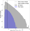 |
Fig. 1. Halo mass distribution for all halos (gray) and halos hosting true pairs (blue). Dashed and dotted lines correspond to the mean (1011.84Mhalo/M⊙ h−1) and median (1011.79Mhalo/M⊙ h−1) values, respectively. |
In Fig. 2 (left panel) we present the total absolute r-band magnitude distribution for the true pairs sample, Mr = −2.5log10(L1 + L2), where L1 (central) and L2 (companion) are the r-band luminosity of the pair members that we compared later to the photometrically identify samples.
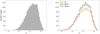 |
Fig. 2. Distribution of the total luminosity for true pairs sample (left) and for the photometrically selected samples (right). SP is the sample with a standard photometric uncertainty (δz = 0.01), and PAUS 1 and PAUS 2 are the two samples with high-precision photometric redshift (δz = 0.002 and δz = 0.0037, respectively). |
The left panel of Fig. 3 shows the distribution of the true pairs luminosity ratio, L2/L1, where a bimodality can be seen with a maximum at 0.25, that is, pairs whose central galaxy is four times brighter than their companion. When the L2/L1 ratios are compared with halo mass of the pairs, we find that pairs with members of similar luminosity tend to reside in halos with higher masses.
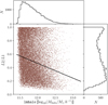 |
Fig. 3. Luminosity ratio of the true pairs members vs. the mass of the halo where the pairs reside. The black line shows the fit of the median values of the L2/L1 obtained in 10 percentiles of halo mass. |
3.2.2. Photometric pairs
After we obtained the true pairs sample, we applied our algorithm to the selected patches of the MICE simulation considering the galaxies with an imposed redshift error that reproduces the photometric data. To mimic the observational catalogs, we added to the z_cgal parameter suitable photometric errors. We defined two samples with high-precision photometric redshift errors that follow the values expected in PAUS, and a third sample, SP, with lower precision standard photometric uncertainties (δz = 0.01).
Following Eriksen et al. (2019), we considered the uncertainties of two samples with high-precision photometric redshift as δz × (1 + z), with δz = 0.002 and δz = 0.0037, labeled PAUS 2 (a better quality sample) and PAUS 1 (which corresponds to the typically expected photo-z precision for PAUS), respectively. We assigned to each galaxy in the samples a photometric redshift, zphot, taken from a Gaussian distribution with z_cgal as the mean and the expected uncertainties as the 1σ standard deviation.
We identify pairs in the three samples with the different redshifts uncertainties taking into account a compromise between purity and completeness for setting the ΔV parameter. In this procedure we simply evaluate that the velocity difference of both galaxies is smaller than the given ΔV value taking into account the assigned photometric redshift zphot (i.e. c|zphot, 1 − zphot, 2| < ΔV).
Purity, P, quantifies the chance of pair members to reside in the same halo:

where Ni is the number of identified pairs in which both members reside in the same halo, and NTrue is the total number of true pairs. Thus, high values of P exclude a significant number of spurious pairs in the photometric selected sample.
On the other hand, the halo completeness, C, quantifies if the halos where true pairs reside are identified as pairs:

where Niden is the total number of identified pairs. C provides information about the total pairs that we can recovered with our procedure.
To set the ΔV threshold for each photometric sample, we tested several values in order to maximize the number of identified pairs with the highest C and P parameters. The general properties of the obtained photometric pair samples are listed in Table 1. With increasing photometric redshift error, completeness is more affected than purity, therefore larger redshift errors tend to lose true pairs at a higher rate rather than including galaxies that reside in different halos.
General properties of the identified photometric pairs samples.
It is important to note that the observational properties of the photometric samples are very similar to those of true pairs in total luminosity distribution and member luminosity ratio (Figs. 2 and 4). Nevertheless, photometric samples tend to include more pairs with higher luminosity than the true pairs, and they have lower L2/L1.
 |
Fig. 4. Ratio between the fraction of pairs selected within L2/L1 bins for each photometric sample, n, and for the true pairs, nTrue. L2/L1 distributions are in excellent agreement with the distributions derived for the true pairs when L2/L1 > 0.2 is considered. It is important to highlight that pairs with L2/L1 < 0.2 constitute ∼10% of all the selected samples. |
4. Lensing analysis
In order to predict the lensing signal associated with the different galaxy pair samples3, we used the lensing properties provided by MICE. We first assess and validate the mass determination for a sample of pure halos binned according to the friends-of-friends (FOF) halo mass. Then, we apply the same analysis to the three photometric redshift galaxy pair samples SP, PAUS 1, and PAUS 1.
We first describe the stacking technique we used to derive total masses. We selected source galaxies, that is, galaxies affected by lensing, taking into account the available shear catalogs in MICE. Then we present the results obtained for the total halo samples and for the galaxy pair samples.
4.1. Stacking techniques
Gravitational lensing distorts the shape of background galaxies that lie behind galaxy systems. The induced shape distortion is quantified by the shear parameter, γ, that can be related to the projected density distribution of the galaxy system. Shear estimates are obtained in observations according to the measured ellipticities of the galaxies. Nevertheless, because galaxies are not intrinsically round, the observed ellipticity is a combination of the intrinsic galaxy ellipticity and the lensing shear effect. The dispersion of intrinsic ellipticities introduces noise in shear estimates, known as “shape noise”, which is proportional to the inverse square root of the number of source galaxies.
Stacking techniques are commonly used to derive the total mass of the composite lenses that are considered (e.g., Leauthaud et al. 2010; Melchior 2013; Rykoff et al. 2008; Foëx et al. 2014; Chalela et al. 2017, 2018; Pereira et al. 2018; Gonzalez et al. 2019). The implementation of this method allowed us to increase the number of source galaxies, which decreases the shape noise and results in better estimates of the total mass. Moreover, the resulting projected density distribution is softened, reducing the effect of the substructures in the halos.
Application of the stacking method consists of the combination of many lenses by averaging the measured distortions of source galaxies. In the case of spherical symmetry, the average of the tangential shear component,  , in an annulus of physical radius, r is related to the projected density contrast,
  , defined as

where  and
and  are the average projected mass distribution within a disk and in a ring of radius r, respectively. Σcrit is the critical density, defined as

which considers the geometrical configuration of the observer-lens-source system through the angular diameter distances between the observer to the source, DOS, the observer to the lens DOL, and the lens to the source DLS. On the other hand, the average of the shear component tilted by π/4, called the cross component,  , should be zero and is used to test for systematic effects.
We combined the lensing signal for a number of lenses, NLenses, and derived the projected density contrast profile by averaging the tangential component of the shear,

where Nsources, j and Ntotal sources are the total number of sources located at a distance r ± δr for the jth lens and for the whole sample of lenses. Σcrit, ij is the critical density for the ith source of the jth lens.
Density contrast profiles were obtained by considering logarithmic equally spaced radial bins, from rin = 350 kpc, taking into account the lensing resolution of MICE v2.0 (pixel_size = 0.43 arcmin), up to rout. The value of rout was computed according to the average halo mass of the lenses in order to avoid the region where the two-halo term becomes significant. For this, we used the relation presented by Simet et al. (2017) between the richness and the upper limit radius combined with their mass-richness relation, taking into account the halo mass provided by MICE. In the case of the galaxy pair samples, we estimated this radius according to this relation and fixed its value to rout = 1.0 Mpc.
4.2. Source galaxy selection
We selected MICE source galaxies taking into account the characteristics of the CFHTLenS survey, which provides weak-lensing catalogs in regions that overlap the PAUS data (CFHTLenS is the reference catalog for PAUS forced-aperture narrow-band photometry that is used to measure accurate photometric redshifts). This survey is based on deep multicolor data, and it spans 154 square degrees distributed in four patches W1, W2, W3, and W4 (63.8, 22.6, 44.2, and 23.3 deg2 respectively). Lensing catalogs include photometric redshift estimates, ZB, computed by Hildebrandt et al. (2012) using the Bayesian photometric redshift software BPZ (Benítez 2000; Coe et al. 2006), which is used for the source galaxy selection. We also applied a cut in the ODDS parameter, a measure of the quality of the redshift estimate. This parameter varies between 0 and 1; galaxy samples with higher ODDS values have a lower fraction of outliers (see, e.g., Eriksen et al. 2019).
We computed the surface density of background galaxies that would be expected based on these lensing catalogs by selecting the galaxies from the CFHTLenS catalog with 0.2 < ZB < 1.3 and with ODDS > 0.5. With these requirements, the source density is ∼7 galaxies arcmin−2 considering the masking regions. Taking these estimates into account, we first selected from the MICE catalog the galaxies with  , which is the CFHTLenS limiting magnitude (Heymans et al. 2012). Then source galaxies were randomly selected in order to obtain the same density as is expected from CFHTLens data at the same redshift range. Each halo at redshift zH was considered as a lens, and we selected the sources as galaxies with z_cgal > zH + 0.1. This last criterion is usually applied in a stacking lensing analysis (Leauthaud et al. 2017; Pereira et al. 2018; Chalela et al. 2018; Gonzalez et al. 2019).
In our analysis, we considered two source galaxy samples, one noisy and the other noise free. For the noisy sample, we simulate the observational noise by adding to the shear a Gaussian random value with zero average ellipticity and dispersion σe = 0.28. This value corresponds to the measured ellipticity dispersion of the CFHTLenS survey, and includes both intrinsic ellipticity dispersion and measurement noise (Simon et al. 2015). On the other hand, the noise-free sample considers the original shear parameters provided by MICE.
Errors in the density contrast profiles based on the noise-free source sample were obtained for each radial bin according to the standard error, considering the dispersion of the individual profiles obtained for all the NLenses halos included in the stacking. In the case of the profiles derived using the noisy source sample, we estimated the error as  , where N is the total number of source galaxies considered in the radial bin.
4.3. Modeling the lensing signal
Halo masses were obtained by fitting the computed contrast density profiles using an NFW density distribution model (Navarro et al. 1997). This profile depends on two parameters, R200, which is the radius that encloses a mean density equal to 200 times the critical density of the Universe, and a dimensionless concentration parameter, c200. This density profile is given by

where ρcrit is the critical density of the Universe at the average redshift of the lenses, rs is the scale radius, rs = R200/c200, and δc is the characteristic overdensity of the halo,

The mass within R200 can be obtained as M200 = 200 ρcrit(4/3)  . Lensing formulae for the NFW density profile were taken from Wright & Brainerd (2000).
There is a well-known degeneracy between R200 and c200 that can only be broken when we consider information about the density distribution in the inner radius. For the profiles based on the noise-free source sample we fit both parameters. We also computed the masses using a fixed mass-concentration relation c200(M200, z), derived from simulations by Duffy et al. (2008),

where we took z as the mean redshift value of the lens sample. In the case of the noisy sample, we only fit R200 and considered the previous Duffy et al. (2008) relation because R200 and c200 cannot be simultaneously constrained given the observed profile uncertainty.
4.4. Lensing results for halos
We applied the described lensing analysis considering as lenses all the halos satisfying the same redshift range as the identified galaxy pairs, 0.2 < z_cgal < 0.6, and with an lmhalo > 11.5 log(M/M⊙). With these criteria the total sample of lenses includes 231 970 halos. We split the sample according to the lmhalo parameter into 15 evenly spaced bins of 0.2 dex width. The profiles we derived for three halo mass bins are shown in Fig. 5.
 |
Fig. 5. Average density contrast profiles for three halo mass bins, from left to right, lmhalo ∈ [12.10,12.30), [12.90,13.10), and [13.70,13.90) log(M/M⊙). The density contrast derived from the noise-free source sample is shown in blue, the best-fit NFW obtained fitting c200 (solid orange line), and fixing it using the relation of Duffy et al. (2008) (dashed green line). Gray points correspond to profiles obtained according to the noisy source sample, and the corresponding best-fit NFW is plotted as the solid gray line. h70 corresponds to h = 0.7. |
We evaluated the derived halo concentrations by comparing the fitted c200 parameter for the profiles obtained by using the noise-free source sample. In Fig. 6 we show the fitted concentration parameters together with those predicted according to the Duffy et al. (2008) relation as a function of halo mass. Concentration values cannot be accurately determined for lmhalo < 12.5 log(M/M⊙). Poorly constrained concentrations can be due to the lack of information in the inner regions of the density profiles. This is more important for low-mass halos because changes in the profile slope corresponding to different concentrations are significant at smaller radii. For lmhalo > 12.5 log(M/M⊙), fitted concentrations tend to be lower than the predicted values. This can be seen from the highest mass bin shown in Fig. 5, where the derived profile from the noise-free source sample flattens at small radius compared to the best-fit NFW model using the Duffy et al. (2008) relation. This result is in agreement with that obtained by López-Arenillas (2014). By analyzing the stacked 3D density profiles of halos in MICE, he derived best-fitting concentrations that are lower than predicted from other literature relations. In spite of the similarity of the cosmological parameters of the MICE and Duffy et al. (2008) simulations, for lmhalo ≧ 13 log(M/M⊙) the fitted concentrations are roughly half of those predicted using the Duffy et al. (2008) relation. These observed differences could be due to a greater softening length of the MICE simulation (lsoft = 50 h−1 kpc, which is 100 times longer than the softening used by Duffy et al. 2008). This can lead to less concentrated halos.
 |
Fig. 6. Derived concentration parameters from the profiles based on the noise-free source sample (dashed gray line) vs. halo masses compared with the concentrations obtained using the Duffy et al. (2008) relation (solid red line). The gray area corresponds to the errors in the fitted concentrations. The red area is computed according to the errors in the parameters of the relation reported by Duffy et al. (2008). Fitted concentrations are well constrained for halos with masses lmhalo > 12.5 log(M/M⊙), but predicted concentrations using the relation by Duffy et al. (2008) are about twice the values obtained by fitting this parameter. |
According to the derived reduced chi-square values (Fig. 7), lensing profiles are well constrained by an NFW model, except for masses lmhalo > 13.5 log(M/M⊙) computed by fixing the concentration parameters using the relation by Duffy et al. (2008).
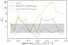 |
Fig. 7. Reduced chi-square values, |

Derived M200 values based on the profiles using the noise-free sample source correlate well with the FOF halo masses, lmhalo, see Fig. 8. We do not expect a one-to-one relation between FoF mass and M200 (White 2001; Jiang et al. 2014). In particular, we find that the estimated lensing mass to lmhalo ratio accurately follows a constant value ∼0.7 in the mass range 11.5 − 13.5 log(M/M⊙). For higher halo masses (lmhalo > 13.5 log(M/M⊙)), lensing masses derived by fitting the concentration parameter are higher than those obtained when this parameter is fixed considering the relation by Duffy et al. (2008). On the other hand, for lower halo masses (where the concentration parameter is poorly constrained), lensing masses have larger uncertainties and are lower than expected when the concentration is fixed.
 |
Fig. 8. Ratio between the derived M200 lensing masses and the FOF halo masses derived from profiles obtained considering the noise-free source sample, fitting the concentration parameter (dashed green line) and considering the Duffy et al. (2008) relation to fit the profile (dashed orange line). |
As shown in Fig. 9, M200 values derived for the noise-free source sample are consistent with those of the noisy sample,  . Nevertheless, the observed signal-to-noise ratio for the noisy source sample drops significantly when halos with masses < 12.5 log(M/M⊙h−1) are considered. Figure 10 shows the relative mass uncertainty as a function of M200 for the noise-free sample. Halos with masses > 12.5 log(M/M⊙h−1) can be detected with high significance. On the other hand, inferred lensing masses for low-mass halos ≲12.0 log(M/M⊙h−1) have a large uncertainty (relative error > 30%). This can also be seen by inspecting the density contrast profiles (Fig. 5). The lensing signal drops significantly below the detection level for low-mass halos, which turns into underestimated masses. Given that the galaxy pairs reside in low-mass halos, (Fig. 1), this effect can hamper the detection of these galaxy systems. This problem is discussed in the next section.
 |
Fig. 9. Ratio between derived lensing masses considering the noisy and the noise-free source samples, taking the relation by Duffy et al. (2008) into account. The shaded region corresponds to the fitted errors in the masses derived according to the noisy source sample. |
4.5. Lensing analysis of galaxy pairs
We computed lensing masses for both the photometric pair and the true pairs samples. By considering the noise-free sources to compute the profiles, we split the pairs according to their total r-band luminosity, Mr, considering bins with an absolute magnitude width of 0.7.
The relation between the derived lensing mass and mean luminosity in each bin is shown in Fig. 11. The correlation between the estimated masses for the true pairs sample and the photometric pairs is good. This result underlines the good performance of our identification algorithm, which can properly recover the observational properties of galaxy pairs located in isolated halos. However, we note that masses are systematically underestimated when larger errors in the photometric redshift are considered for galaxy pairs with total absolute magnitudes Mr ≳ −21.5.
Reliable lensing masses from the noisy source sample can only be obtained when galaxy pairs with high luminosity, Mr ≲ −21, are considered. When the relation between the total absolute magnitude and halo mass lmhalo (Fig. 11) is taken into account, this threshold ensures that the masses are well constrained considering the results presented in Fig. 10. Therefore only high-luminosity pairs can be detected with sufficient sensitivity when the observational limitations are taken into account. For these high-luminosity pairs we can recover the slope of the M200 − Mr relation when the photometric samples are taken into account.
 |
Fig. 10. Lensing mass relative errors |

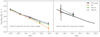 |
Fig. 11. Derived lensing masses for the different pair samples vs. the average total magnitude of the pairs in the considered bin. Left panel: result obtained by stacking the noise-free source sample (solid lines). Right panel: same relation as dashed lines for the masses obtained from the noisy source sample and as the solid line for comparison the same relation as in the left panel obtained for the true pairs sample. For the higher magnitude bin in the case of the SP sample, we were unable to constrain the mass properly. |
For the highest luminosity bin of the true pairs sample, we obtain a larger uncertainty due to the low number of pairs in this bin. Because it uses a low number of sources, the stacking procedure lacks effectiveness in providing suitable mass estimates. We note, however, that the general trend of the mass-luminosity relation is well recovered.
We have also explored the dependence of the mass-luminosity relation by adopting different selection criteria for the pair samples taking the redshift, color, and luminosity ratio of member galaxies into account, see Fig. 12. We find no difference in the mass-luminosity relation for samples selected according to the median redshift of the sample pairs (z = 0.41), as shown in the left panel of Fig. 12. We classified the pairs into red and blue based on the redshift and absolute magnitude bins of the member galaxies. We found no significant differences between the red and blue populations (see Fig. 12 middle panel). This result contrasts with the finding of Gonzalez et al. (2019), who obtained that red pairs have higher lensing masses. Further analysis needs to be performed in order to determine whether these discrepancies can be explained by a color-density dependence difference between the simulation and the observations. Galaxy luminosities and colors are assigned in the MICE mock catalog in order to match observed galaxy properties and the clustering dependence on these parameters (Carretero et al. 2015). In particular, galaxy colors are assigned to fit the observed (g − r) versus Mr SDSS observed relation (Blanton et al. 2003) and the clustering properties as a function of color (Zehavi et al. 2011). The procedure is similar to the model presented in Skibba & Sheth (2009), in which colors depend on galaxy type (whether it is a central or a satellite galaxy), and on its color sequence (red, blue, and green), but not on the parent halo mass. First, colors are assigned to the satellite galaxies considering their absolute magnitudes to set the fraction of satellite galaxies that belongs to the red and green sequences. Because the systems analyzed in this work reside in low-mass halos, the number of expected satellites is small and a high uncertainty is therefore expected in its color assignment, leading to possible discrepancies with observed colors for these particular systems.
 |
Fig. 12. Derived lensing masses for all the true pairs vs. the average total magnitude of the pairs in the considered bin obtained according to the noise-free source sample. In red and blue we show the same relation, but splitting the true pairs according to the pair redshift (left panel), color (middle panel), and luminosity ratio of the galaxy members. |
We note, however, that the results of Gonzalez et al. (2019) may be explained by the inclusion of unbound systems in the blue sample of pairs, resulting in lower derived lensing masses. In the right panel of Fig. 12, we explore the dependence of the total mass-luminosity relation of the pairs selected according to the pair member luminosity ratio, L2/L1. The estimated lensing masses are about twice lower for pairs with similar luminosity members. Although this result cannot be tested with the present observational data because the masses are poorly estimated when noise is considered, this result could be addressed with better quality data in future surveys.
5. Summary and conclusions
We presented an algorithm for the identification of galaxy pairs based on photometric information. The identification algorithm successfully reproduces the distribution of total luminosity and mass of truly bound galaxy pairs residing in the same dark matter halo. Pairs were identified through a commonly used procedure: adopted fixed values of projected separation rp and relative velocities ΔV, plus the requirement that all systems have at least one bright member (Mr < −19.5) and that the pair members have an apparent magnitude difference Δm < 2. Finally, we applied an isolation criterion that allowed us to exclude pairs in massive systems. The algorithm was applied to three galaxy samples from the MICE simulation that consider different photometric redshift uncertainties, and derive three catalogs of photometric pairs in the redshift range 0.2 − 0.6.
In order to test our identification algorithm, we selected galaxy pairs that met all the criteria described above. Additionally, both galaxy members resided in the same halo. This was called the true pairs sample. This restriction provides a novel approach to testing galaxy pair identification techniques. Then, we compared the recovered photometric pairs with the true pairs. As expected, we find that the identification reliability improves as the photometric redshift error decreases. Nevertheless, all the pair samples identified based on photometric data properly recover the distribution of observational properties of the true pairs: total luminosity and pair member luminosity ratio. The derived luminosity ratio of the photometric pair members shows a bimodal behavior. We also find that pairs with similar luminosity members (higher luminosity ratios) tend to reside in more massive halos at a given total pair luminosity. As the accuracy in the photometric redshift error improves, galaxy pair samples tend to recover more systems that are classified as true pairs. This ensures that PAUS will provide a valuable contribution to the identification of galaxy systems.
We have also studied the different pair samples using weak-lensing techniques. In order to test the performance of our lensing analysis and its ability to recover total halo masses, we first analyzed a sample of halos within the same redshift range as the pairs, and with halo masses higher than > 11.5 log(M/M⊙). Source galaxies were selected considering the CFHTLenS data properties in order to mimic observational conditions. Lensing masses were obtained by applying stacking techniques by splitting the total halo sample into different halo mass bins. We find that the derived density contrast profiles of higher mass halos are less concentrated than predicted by Duffy et al. (2008). For lower mass halos, the lensing analysis cannot properly constrain the halo concentration parameter. Nevertheless, the derived M200 strongly correlates with the total halo FOF masses provided by MICE. When source samples are considered to which lensing properties have added observational noise, the concentration parameter cannot be accurately determined, but the derived M200 agrees excellently well with the values obtained without observational noise. However, the signal-to-noise ratio drops significantly when halos with masses < 12 log(M/M⊙) are considered.
Although lensing masses tend to be systematically underestimated for the samples with larger photo-z errors, in general, masses for all the identified samples are successfully recovered with our analysis. Even when observational noise is considered for the lensing analysis, we can successfully recover the slope of the lensing mass versus total luminosity relation. However, masses can be determined only for galaxy pairs with total absolute r-band magnitudes brigther than −21. This luminosity threshold roughly corresponds to galaxy pairs in halos with masses > 12.5 log(M/M⊙). When galaxy pairs are considered that are identified using standard photometric redshift uncertainties (i.e., a factor 2.7 higher than the typical error predicted for PAUS), the lensing signal is lowered because fewer galaxy pairs are identified. For this photometrically selected sample, lensing masses can only be recovered for the most luminous pairs. It is important to highlight that although the selection criteria for the galaxy pair identification can be relaxed by considering larger limits for ΔV or Δm, this would result in a decrease in the purity of the selected sample but would not improve the lensing signal.
The results we obtained show that the upcoming PAUS data with high-quality photometric redshift information will enable the construction of large and reliable samples of galaxy systems. Identifying isolated galaxy pairs is a challenging task because these low-mass systems can only be detected based on a few photometric parameters. It is therefore important to apply accurate tests that ensure the recovery of truly bound systems. Our algorithm allows us to collect suitable samples that can be used to obtain physical properties that lead to a deeper understanding of their formation and evolution in a cosmological context.
Acknowledgments
We thank the anonymous referee for his/her comments that helped to improve this work. We thank Carlton Baugh for his careful reading of the manuscript that has helped us to improve the text. This project has received funding from the European Union’s Horizon 2020 Research and Innovation Programme under the Marie Sklodowska-Curie grant agreement No 734374. This work has been supported by MINECO grants AYA2015-71825 & ESP2015-66861. IEEC is partially funded by the CERCA program of the Generalitat de Catalunya. This work was also partially supported by Agencia Nacional de Promoción Científica y Tecnoóogica (PICT 2015-3098), the Consejo Nacional de Investigaciones Científicas y Técnicas (CONICET, Argentina) and the Secretaría de Ciencia y Tecnología de la Universidad Nacional de Córdoba (SeCyT-UNC, Argentina). MS has been supported by the European Union’s Horizon 2020 research and innovation programme under the Maria Skłodowska-Curie grant agreement No 754510 and National Science Centre (grant UMO-2016/23/N/ST9/02963). MM acknowledges support from the Beatriu de Pinos fellowship (2017-BP-00114). We made an extensive use of the following python libraries: http://www.numpy.org/, http://www.scipy.org/, https://www.astropy.org/ and http://www.matplotlib.org/. This work has made use of CosmoHub. CosmoHub has been developed by the Port d’Informació Científica (PIC), maintained through a collaboration of the Institut de Física d’Altes Energies (IFAE) and the Centro de Investigaciones Energéticas, Medioambientales y Tecnológicas (CIEMAT), and was partially funded by the “Plan Estatal de Investigación Científica y T’ecnica y de Innovación” program of the Spanish government. EJG and FR would like to specially thank the contribution of Darío Graña who helped to run the algorithms. Gracias por las picadas. Go team Barcelona! EJG, FR and AO thank Orion for the laughter and the good luck.
References
- Benítez, N. 2000, ApJ, 536, 571 [NASA ADS] [CrossRef] [Google Scholar]
- Blanton, M. R., Hogg, D. W., Bahcall, N. A., et al. 2003, ApJ, 594, 186 [NASA ADS] [CrossRef] [Google Scholar]
- Carretero, J., Castander, F. J., Gaztañaga, E., Crocce, M., & Fosalba, P. 2015, MNRAS, 447, 646 [NASA ADS] [CrossRef] [Google Scholar]
- Carretero, J., Tallada, P., Casals, J., et al. 2017, PoS (EPS-HEP2017), 314, 488 [Google Scholar]
- Chalela, M., Gonzalez, E. J., Garcia Lambas, D., & Foex, G. 2017, MNRAS, 467, 1819 [NASA ADS] [Google Scholar]
- Chalela, M., Gonzalez, E. J., Makler, M., et al. 2018, MNRAS, 479, 1170 [NASA ADS] [CrossRef] [Google Scholar]
- Chamaraux, P., & Nottale, L. 2016, Astrophys. Bull., 71, 270 [Google Scholar]
- Chengalur, J. N., Salpeter, E. E., & Terzian, Y. 1996, ApJ, 461, 546 [NASA ADS] [CrossRef] [Google Scholar]
- Coe, D., Benítez, N., Sánchez, S. F., et al. 2006, AJ, 132, 926 [NASA ADS] [CrossRef] [Google Scholar]
- Crocce, M., Castander, F. J., Gaztañaga, E., Fosalba, P., & Carretero, J. 2015, MNRAS, 453, 1513 [NASA ADS] [CrossRef] [Google Scholar]
- Dietrich, J. P., Werner, N., Clowe, D., et al. 2012, Nature, 487, 202 [Google Scholar]
- Duffy, A. R., Schaye, J., Kay, S. T., & Dalla Vecchia, C. 2008, MNRAS, 390, L64 [NASA ADS] [CrossRef] [Google Scholar]
- Ellison, S. L., Patton, D. R., Simard, L., et al. 2010, MNRAS, 407, 1514 [NASA ADS] [CrossRef] [Google Scholar]
- Eriksen, M., Alarcon, A., Gaztanaga, E., et al. 2019, MNRAS, 484, 4200 [Google Scholar]
- Faber, S. M., & Gallagher, J. S. 1979, ARA&A, 17, 135 [NASA ADS] [CrossRef] [MathSciNet] [Google Scholar]
- Ferreras, I., Hopkins, A. M., Gunawardhana, M. L. P., et al. 2017, MNRAS, 468, 607 [NASA ADS] [CrossRef] [Google Scholar]
- Ferreras, I., Hopkins, A. M., Lagos, C., et al. 2019, MNRAS, 487, 435 [NASA ADS] [CrossRef] [Google Scholar]
- Foëx, G., Motta, V., Jullo, E., Limousin, M., & Verdugo, T. 2014, A&A, 572, A19 [NASA ADS] [CrossRef] [EDP Sciences] [Google Scholar]
- Fosalba, P., Gaztañaga, E., Castander, F. J., & Manera, M. 2008, MNRAS, 391, 435 [NASA ADS] [CrossRef] [Google Scholar]
- Fosalba, P., Crocce, M., Gaztañaga, E., & Castander, F. J. 2015a, MNRAS, 448, 2987 [NASA ADS] [CrossRef] [Google Scholar]
- Fosalba, P., Gaztañaga, E., Castander, F. J., & Crocce, M. 2015b, MNRAS, 447, 1319 [NASA ADS] [CrossRef] [Google Scholar]
- Gao, L., Springel, V., & White, S. D. M. 2005, MNRAS, 363, L66 [NASA ADS] [CrossRef] [Google Scholar]
- Gonzalez, E. J., de los Rios, M., Oio, G. A., et al. 2018, A&A, 611, A78 [NASA ADS] [CrossRef] [EDP Sciences] [Google Scholar]
- Gonzalez, E. J., Rodriguez, F., García Lambas, D., et al. 2019, A&A, 621, A90 [NASA ADS] [CrossRef] [EDP Sciences] [Google Scholar]
- Guhathakurta, P. 2003, Discoveries and Research Prospects from 6- to 10-Meter-Class Telescopes II, 4834 [Google Scholar]
- Hernández-Toledo, H. M., Avila-Reese, V., Conselice, C. J., & Puerari, I. 2005, AJ, 129, 682 [NASA ADS] [CrossRef] [Google Scholar]
- Heymans, C., Van Waerbeke, L., Miller, L., et al. 2012, MNRAS, 427, 146 [NASA ADS] [CrossRef] [Google Scholar]
- Hildebrandt, H., Erben, T., Kuijken, K., et al. 2012, MNRAS, 421, 2355 [NASA ADS] [CrossRef] [Google Scholar]
- Jauzac, M., Jullo, E., Kneib, J.-P., et al. 2012, MNRAS, 426, 3369 [Google Scholar]
- Jian, H.-Y., Lin, L., & Chiueh, T. 2012, ApJ, 754, 26 [NASA ADS] [CrossRef] [Google Scholar]
- Jiang, L., Helly, J. C., Cole, S., & Frenk, C. S. 2014, MNRAS, 440, 2115 [NASA ADS] [CrossRef] [Google Scholar]
- Jullo, E., Pires, S., Jauzac, M., & Kneib, J. P. 2014, MNRAS, 437, 3969 [NASA ADS] [CrossRef] [Google Scholar]
- Kitzbichler, M. G., & White, S. D. M. 2008, MNRAS, 391, 1489 [NASA ADS] [CrossRef] [Google Scholar]
- Lambas, D. G., Tissera, P. B., Alonso, M. S., & Coldwell, G. 2003, MNRAS, 346, 1189 [NASA ADS] [CrossRef] [Google Scholar]
- Lambas, D. G., Alonso, S., Mesa, V., & O’Mill, A. L. 2012, A&A, 539, A45 [NASA ADS] [CrossRef] [EDP Sciences] [Google Scholar]
- Leauthaud, A., Finoguenov, A., Kneib, J. P., et al. 2010, ApJ, 709, 97 [NASA ADS] [CrossRef] [Google Scholar]
- Leauthaud, A., Saito, S., Hilbert, S., et al. 2017, MNRAS, 467, 3024 [NASA ADS] [CrossRef] [Google Scholar]
- Lilly, S. J., Le Fèvre, O., Renzini, A., et al. 2007, ApJS, 172, 70 [NASA ADS] [CrossRef] [Google Scholar]
- Lin, L., Koo, D. C., Willmer, C. N. A., et al. 2004, ApJ, 617, L9 [NASA ADS] [CrossRef] [Google Scholar]
- López-Arenillas, C. 2014, PhD Thesis, Universitat de Barcelona [Google Scholar]
- López-Sanjuan, C., Cenarro, A. J., Varela, J., et al. 2015, A&A, 576, A53 [NASA ADS] [CrossRef] [EDP Sciences] [Google Scholar]
- Melchior, P. 2013, SnowCLUSTER 2013, Physics of Galaxy Clusters, held 24–19 March, 2013 at the University of Utah, 52 [Google Scholar]
- Mesa, V., Duplancic, F., Alonso, S., Coldwell, G., & Lambas, D. G. 2014, MNRAS, 438, 1784 [NASA ADS] [CrossRef] [Google Scholar]
- Miller, L., Heymans, C., Kitching, T. D., et al. 2013, MNRAS, 429, 2858 [Google Scholar]
- Moreno, J., Bluck, A. F. L., Ellison, S. L., et al. 2013, MNRAS, 436, 1765 [NASA ADS] [CrossRef] [Google Scholar]
- Navarro, J. F., Frenk, C. S., & White, S. D. M. 1997, ApJ, 490, 493 [NASA ADS] [CrossRef] [Google Scholar]
- Niemi, S.-M., Kitching, T. D., & Cropper, M. 2015, MNRAS, 454, 1221 [NASA ADS] [CrossRef] [Google Scholar]
- Norberg, P., Frenk, C. S., & Cole, S. 2008, MNRAS, 383, 646 [NASA ADS] [CrossRef] [Google Scholar]
- Nottale, L., & Chamaraux, P. 2018, Astrophys. Bull., 73, 310 [NASA ADS] [CrossRef] [Google Scholar]
- Padilla, C., Castander, F. J., Alarcón, A., et al. 2019, AJ, 157, 246 [NASA ADS] [CrossRef] [Google Scholar]
- Patton, D. R., Carlberg, R. G., Marzke, R. O., et al. 2000, ApJ, 536, 153 [NASA ADS] [CrossRef] [Google Scholar]
- Patton, D. R., Qamar, F. D., Ellison, S. L., et al. 2016, MNRAS, 461, 2589 [NASA ADS] [CrossRef] [Google Scholar]
- Pereira, M. E. S., Soares-Santos, M., Makler, M., et al. 2018, MNRAS, 474, 1361 [NASA ADS] [CrossRef] [Google Scholar]
- Peterson, S. D. 1979, ApJS, 40, 527 [NASA ADS] [CrossRef] [Google Scholar]
- Rykoff, E. S., Evrard, A. E., McKay, T. A., et al. 2008, MNRAS, 387, L28 [NASA ADS] [Google Scholar]
- Simet, M., McClintock, T., Mandelbaum, R., et al. 2017, MNRAS, 466, 3103 [NASA ADS] [CrossRef] [Google Scholar]
- Simon, P., Semboloni, E., van Waerbeke, L., et al. 2015, MNRAS, 449, 1505 [NASA ADS] [CrossRef] [Google Scholar]
- Skibba, R. A., & Sheth, R. K. 2009, MNRAS, 392, 1080 [NASA ADS] [CrossRef] [Google Scholar]
- Toomre, A., & Toomre, J. 1972, ApJ, 178, 623 [NASA ADS] [CrossRef] [Google Scholar]
- Umetsu, K., Medezinski, E., Nonino, M., et al. 2014, ApJ, 795, 163 [NASA ADS] [CrossRef] [Google Scholar]
- Wegner, G. A., & Heymans, C. E. 2011, Am. Astron. Soc. Meet. Abstr., 218, 319.04 [NASA ADS] [Google Scholar]
- White, M. 2001, A&A, 367, 27 [NASA ADS] [CrossRef] [EDP Sciences] [Google Scholar]
- Woods, D. F., & Geller, M. J. 2007, AJ, 134, 527 [NASA ADS] [CrossRef] [Google Scholar]
- Wright, C. O., & Brainerd, T. G. 2000, ApJ, 534, 34 [NASA ADS] [CrossRef] [Google Scholar]
- Zehavi, I., Zheng, Z., Weinberg, D. H., et al. 2011, ApJ, 736, 59 [NASA ADS] [CrossRef] [Google Scholar]
All Tables
All Figures
|
Fig. 1. Halo mass distribution for all halos (gray) and halos hosting true pairs (blue). Dashed and dotted lines correspond to the mean (1011.84Mhalo/M⊙ h−1) and median (1011.79Mhalo/M⊙ h−1) values, respectively. |
| In the text | |
|
Fig. 2. Distribution of the total luminosity for true pairs sample (left) and for the photometrically selected samples (right). SP is the sample with a standard photometric uncertainty (δz = 0.01), and PAUS 1 and PAUS 2 are the two samples with high-precision photometric redshift (δz = 0.002 and δz = 0.0037, respectively). |
| In the text | |
|
Fig. 3. Luminosity ratio of the true pairs members vs. the mass of the halo where the pairs reside. The black line shows the fit of the median values of the L2/L1 obtained in 10 percentiles of halo mass. |
| In the text | |
|
Fig. 4. Ratio between the fraction of pairs selected within L2/L1 bins for each photometric sample, n, and for the true pairs, nTrue. L2/L1 distributions are in excellent agreement with the distributions derived for the true pairs when L2/L1 > 0.2 is considered. It is important to highlight that pairs with L2/L1 < 0.2 constitute ∼10% of all the selected samples. |
| In the text | |
|
Fig. 5. Average density contrast profiles for three halo mass bins, from left to right, lmhalo ∈ [12.10,12.30), [12.90,13.10), and [13.70,13.90) log(M/M⊙). The density contrast derived from the noise-free source sample is shown in blue, the best-fit NFW obtained fitting c200 (solid orange line), and fixing it using the relation of Duffy et al. (2008) (dashed green line). Gray points correspond to profiles obtained according to the noisy source sample, and the corresponding best-fit NFW is plotted as the solid gray line. h70 corresponds to h = 0.7. |
| In the text | |
|
Fig. 6. Derived concentration parameters from the profiles based on the noise-free source sample (dashed gray line) vs. halo masses compared with the concentrations obtained using the Duffy et al. (2008) relation (solid red line). The gray area corresponds to the errors in the fitted concentrations. The red area is computed according to the errors in the parameters of the relation reported by Duffy et al. (2008). Fitted concentrations are well constrained for halos with masses lmhalo > 12.5 log(M/M⊙), but predicted concentrations using the relation by Duffy et al. (2008) are about twice the values obtained by fitting this parameter. |
| In the text | |
|
Fig. 7. Reduced chi-square values, |
| In the text | |
|
Fig. 8. Ratio between the derived M200 lensing masses and the FOF halo masses derived from profiles obtained considering the noise-free source sample, fitting the concentration parameter (dashed green line) and considering the Duffy et al. (2008) relation to fit the profile (dashed orange line). |
| In the text | |
|
Fig. 9. Ratio between derived lensing masses considering the noisy and the noise-free source samples, taking the relation by Duffy et al. (2008) into account. The shaded region corresponds to the fitted errors in the masses derived according to the noisy source sample. |
| In the text | |
|
Fig. 10. Lensing mass relative errors |
| In the text | |
|
Fig. 11. Derived lensing masses for the different pair samples vs. the average total magnitude of the pairs in the considered bin. Left panel: result obtained by stacking the noise-free source sample (solid lines). Right panel: same relation as dashed lines for the masses obtained from the noisy source sample and as the solid line for comparison the same relation as in the left panel obtained for the true pairs sample. For the higher magnitude bin in the case of the SP sample, we were unable to constrain the mass properly. |
| In the text | |
|
Fig. 12. Derived lensing masses for all the true pairs vs. the average total magnitude of the pairs in the considered bin obtained according to the noise-free source sample. In red and blue we show the same relation, but splitting the true pairs according to the pair redshift (left panel), color (middle panel), and luminosity ratio of the galaxy members. |
| In the text | |
Current usage metrics show cumulative count of Article Views (full-text article views including HTML views, PDF and ePub downloads, according to the available data) and Abstracts Views on Vision4Press platform.
Data correspond to usage on the plateform after 2015. The current usage metrics is available 48-96 hours after online publication and is updated daily on week days.
Initial download of the metrics may take a while.