| Issue |
A&A
Volume 634, February 2020
|
|
|---|---|---|
| Article Number | A17 | |
| Number of page(s) | 13 | |
| Section | Astrophysical processes | |
| DOI | https://doi.org/10.1051/0004-6361/201936536 | |
| Published online | 29 January 2020 | |
Tracing shock type with chemical diagnostics
An application to L1157
1
Department of Physics and Astronomy, University College London, Gower Street, London WC1E 6BT, UK
e-mail: tjames@star.ucl.ac.uk; t.james.17@ucl.ac.uk
2
Centro de Astrobiologia (CSIC, INTA), Ctra. de Ajalvir, km. 4, Torrejón de Ardoz 28850, Madrid, Spain
Received:
20
August
2019
Accepted:
4
December
2019
Aims. The physical structure of a shock wave may take a form unique to its shock type, implying that the chemistry of each shock type is unique as well. We aim to investigate the different chemistries of J-type and C-type shocks in order to identify unique molecular tracers of both shock types. We apply these diagnostics to the protostellar outflow L1157 to establish whether the B2 clump could host shocks exhibiting type-specific behaviour. Of particular interest is the L1157-B2 clump, which has been shown to exhibit bright emission in S-bearing species and HNCO.
Methods. We simulate, using a parameterised approach, a planar, steady-state J-type shock wave using UCLCHEM. We compute a grid of models using both C-type and J-type shock models to determine the chemical abundance of shock-tracing species as a function of distance through the shock and apply it to the L1157 outflow. We focus on known shock-tracing molecules such as H2O, HCN, and CH3OH.
Results. We find that a range of molecules including H2O and HCN have unique behaviour specific to a J-type shock, but that such differences in behaviour are only evident at low vs and low nH. We find that CH3OH is enhanced by shocks and is a reliable probe of the pre-shock gas density. However, we find no difference between its gas-phase abundance in C-type and J-type shocks. Finally, from our application to L1157, we find that the fractional abundances within the B2 region are consistent with both C-type and J-type shock emission.
Key words: astrochemistry / evolution / ISM: individual objects: L1157 / ISM: molecules / stars: protostars
© ESO 2020
1. Introduction
Astrophysical shocks represent prominent catalysts for chemical evolution in the interstellar medium (ISM). The low signal-speed within the ambient ISM leads to a variety of different astrophysical events driving supersonic flows that form shocks, from cloud-cloud collisions (e.g. Gidalevich 1966) to bipolar outflows emanating from protostellar objects (e.g. Snell et al. 1980; Shu et al. 1991; Zhang & Zheng 1997). The different ambient gas conditions that a supersonic flow can be driven into leads to the production of different shock types. Draine (1980) initially defined two shock types, C (continuous) type shock and J (jump) type shock, with subsequent computational work by Chièze et al. (1998) and Flower et al. (2003a) defining a third, CJ (mixed) type shock.
Unlike C-type shocks, which typically arise in regions with a magnetic field and low degree of fractional-ionisation, J-type shocks arise in regions whereby only a negligible magnetic field is present (Draine 1980). The negligible magnetic field within a J-type shock has further consequences in that it does not act to limit the compression through the shock, thus allowing a higher peak temperature to be reached within the shock-front (relative to a C-type shock). Owing to this, J-type shocks are thought to exhibit far more destructive chemistry than a C-type shock counterpart. An analytic description of a C-type shock therefore requires equations of magnetohydrodynamics (MHD) and multiple fluid components, whilst J-type shocks can be described by hydrodynamics equations and a single fluid alone.
Typically, such descriptions are implemented in MHD codes such as mhd_vode (Flower & Des ForÉts 2015). However, such approaches to modelling incur a large amount of computational expense, necessitating compromises in the complexity and size of the chemical network used. By using a parameterised form of the physical structure of the shock, as Jiménez-Serra et al. (2008) did with their C-type shock parameterisation, it is possible to preserve an approximation of the shock structure whilst significantly reducing computational complexity, thus allowing the computation of far more complex chemistry.
This is particularly important owing to the complex chemistry that is influenced by shocks. In particular, shocks can drive chemical reactions that would otherwise be highly unlikely to occur under quiescent ISM conditions. For example, the reaction O + H2 → OH + H has an activation barrier of ≈1 eV and would therefore require temperatures > 1000 K, which are easily achievable within shocks, to initiate (Baulch et al. 1992; van Dishoeck et al. 2013; Williams & Viti 2013).
It is through such reactions that the axiom of unique chemistry as a diagnostic of prior physical events is drawn. Further reinforcing this axiom is interstellar chemistry’s high density and temperature dependence, thus rendering the composition of the ISM highly sensitive to dynamical environmental effects. Shocks are ubiquitous sources of such change within the ISM, and therefore represent prominent sources of chemical enrichment in early star-forming environments.
Observations of shocked regions allow effective probes of the shock chemistry. Recent high-resolution spectroscopy programmes such as ASAI (Lefloch et al. 2018), CHESS (Lefloch et al. 2010), and WISH (van Dishoeck et al. 2010) permit unprecedented insight into not just early stages of star formation, but also the violent events that initially drive shocks into these regions. The bipolar outflow in L1157 (Umemoto et al. 1992) is an example of a prototypical protostellar outflow observed during these programmes. Observations of outflows cannot, however, provide insight into either the physical or subsequent chemical evolution of the shock through time, instead only capturing a static snapshot of the conditions. Modelling shock-induced chemistry is therefore one of the only methods of following the evolution of an inherently time-dependent chemical process in astrophysics.
The role that dust grains play in interstellar chemistry is also of paramount importance. Molecules in the gas-phase may freeze on to the surface of dust grains, thereby depleting their gas-phase abundance by changing state. Processes such as successive hydrogenation on dust grains are thought to be the mechanism responsible for such complex organic molecule formation as CH3OH (Tielens & Whittet 1997; Fuchs et al. 2009). Importantly this method also presents a viable solution to the cold gas-phase abundance problem whereby molecules are observed in the gas phase at temperatures well below their gas-phase formation temperature. Under the influence of a sputtering, grain-grain collision or desorption event (thermal or non-thermal), the molecule may be released from the surface of the dust-grain directly into the gas phase. This complex interplay between the gas-phase and dust-grain chemistry essentially chemically couples the two phases. It is therefore vitally important when modelling interstellar chemistry that both gas-phase and dust-grain reactions included within the reaction network are accurate and comprehensive for the relevant molecules.
In practice, the only way one can hope to distinguish between the two types of shock is to systematically determine the effects of each shock type and hence compare the resultant chemical distinctions. Our goal in this paper is to identify molecular tracers of a J-type shock by using such a technique and apply it to a shocked region of L1157 thought to be exhibiting signatures of both C-type and J-type shock behaviour. We therefore make extensive use of the C-type shock module, based on Jiménez-Serra et al. (2008), that is already implemented in UCLCHEM (Holdship et al. 2017). To that goal, we present in Sect. 2 an overview of L1157. We present in Sect. 3 a parameterised model of a J-type shock built for the astrochemical code UCLCHEM. In conjunction with the pre-existing C-type shock model based upon Jiménez-Serra et al. (2008) we investigate in Sect. 4 the chemical distinctions between J-type and C-type shocks to identify unique chemical tracers of both shock types. Section 5 applies these results by comparing them to enhanced abundances with shocked regions of the L1157 outflow.
2. L1157
At 250 pc (Looney et al. 2007), L1157 is a nearby region that comprises a central class-0 protostar, L1157-mm, that in turn drives a bipolar outflow. The observed outflow produces a red-shifted lobe to the North and a blue-shifted lobe to the South that are aligned with the protostar’s rotation axis. A degree of symmetry is observed in these lobes, however the geometry of lobe sub-structure indicates the presence of an underlying precessing jet (Vasta et al. 2012). This precession allows periodic ejection events to create complex structures enhanced by shocks (Gueth et al. 1996). The Southern lobe hosts two intriguing examples of such shock events: the clumps B1 and B2, which are themselves located within larger cavities C1 and C2. As a result, L1157 is considered to be one of the best laboratories for astrochemistry (Umemoto et al. 1992; Bachiller et al. 2001).
Figure 1 shows Spitzer/IRAC 8 μm observations by Podio et al. (2016). Labelled are the knots B0, B1 and B2 alongside the central driving protostar L1157-mm and the proposed precession model from Podio et al. (2016).
 |
Fig. 1. Spitzer/IRAC 8 μm image of the L1157 outflow. (Podio et al. 2016). Shown as black squares are the shock events B0, B1 and B2. The class-0 protostar L1157-mm that drives the outflow is also labelled. The black line overplotted is the precession model thought to be responsible for the creation of the observed knots. As is visible here, B2 is far less intense in emission than B0/B1. |
It has since been found that B1 and B2 themselves host low-velocity clumps. Benedettini et al. (2007), using PdB interferometric observations, showed that nine clumps exist within the B1 and B2 structure, thus giving rise to even further complexity within the Southern lobe. This substructure is thought to arise from L1157-mm’s precession, which creates complex knots driven by shock-activity produced by the host outflow.
2.1. L1157-B1
B1 is the brightest clump within the L1157 region and thus the subject of significant study. It is warm and young, exhibiting kinetic temperatures between T ≈ 80−100 K and age t ≈ 1000 years. In comparison B2 is colder and older with T ≈ 20−60 K and t ≈ 4000 years (Tafalla & Bachiller 1995; Gueth et al. 1996). Viti et al. (2011) first showed, with confirmation by Benedettini et al. (2012), that B1 is likely produced by a non-dissociative, C-type shock with pre-shock density nH ≥ 104 cm−3 and vs ≈ 40 km s−1, leading to a maximum obtainable temperature of ∼4000 K.
2.2. L1157-B2
Being less intense in most emission lines, B2 has been subject to far less study. B2 is, however, brighter than B1 in most sulphur-bearing species as well as HNCO (Tafalla & Bachiller 1995; Bachiller & Pérez Gutiérrez 1997; Rodríguez-Fernández et al. 2010). Tafalla & Bachiller (1995) specifically finds that SO and SO2 exhibit enhancement factors within L1157-B2 (relative to L1157-mm) of between 60−100 and 20, respectively. Meanwhile, they also find that the enhancement factors for L1157-B1 are 50−70 and 8. HNCO is thought to form efficiently on grain surfaces, whilst S-bearing species like SO and SO2 form in the gas-phase with sputtered S from the grains themselves (Allen & Robinson 1977; Charnley 1997; Garrod et al. 2008). The older dynamical age of B2 relative to B1 could lend credence to the idea that B2 has simply had more time than B1 to chemically process the sputtered material, hence the more luminous species like HNCO and S-bearing species. Table 1 lists further molecules observed within L1157 and their enhancement factors, where fenhance = χ(R)/χ(0). Importantly these enhancement factors, as well as their associated abundances, are subject to large uncertainties arising from the assumption that the observed lines are both optically thin and thermalised.
Abundances χ of known shock enhanced molecules and their enhancement factors f (relative to χ(0)) in the two L1157 knots B1 and B2.
To date studies such as those by Vasta et al. (2012) have not yet been able to determine with certainty the prevalent shock type within B2, though Vasta et al. (2012) does allude to the possibility of a J-type shock component within L1157-B2. Gómez-Ruiz et al. (2016) use NH3 and H2O abundances, alongside model predictions, to trace shock temperature within L1157’s lobes. Gómez-Ruiz et al. (2016) finds that whilst a proper line radiative transfer model is needed for proper computation, the best matching model for L1157-B2 is one with nH ≈ 103 cm−3 and vs ≈ 10 km s−1.
3. Shock modelling
Our parameterised model is based on the MHD code mhd_vode (Flower & Des ForÉts 2015). mhd_vode is an ideal-MHD, 1D, two-fluid simulation of both C-type and J-type shocks that computes chemistry in parallel with its physics. This model is built as a module to the time-dependent chemical code UCLCHEM (Holdship et al. 2017).
UCLCHEM is a diverse code, and its modularised functionality lends itself to a host of different astrochemical problems and environments. For a full description of UCLCHEM’s operation see Holdship et al. (2017) as well as the documentation hosted online1. In brief, UCLCHEM is constructed so as to follow a two-phase computation. Firstly an ambient medium of user-supplied temperature, density and chemical composition undergoes an isothermal collapse as described by Rawlings et al. (1992) to a user-supplied final density. The chemical composition of a 1D parcel is therefore followed during collapse, and thus informs the chemical conditions for phase 2. During phase 2, the relevant physics supplied via a user module is computed and used to inform the rates of reactions within the chemical network. Our J-type shock module is built so as to follow this methodology.
3.1. J-type shock parameterisation
To construct our parameterised model we first noted that, as described by Zel’dovich & Raizer (1967), shocks can generally be discretised into four regions: the precursor, the shock-front, the post-shock relaxation layer and the thermalisation layer. We neglect the radiative precursor component of the shock in our models, as J-type shocks with vs < 80 km s−1 have been found to have negligible radiative precursor components, therefore playing no role in either the shock structure or the shock chemistry (Hollenbach & McKee 1989; Flower et al. 2003b). We also neglect the thermalisation layer, instead focusing on the shock-front and the post-shock relaxation layer as sole sources of chemical evolution. We assume that the post-shock gas cools to its initial temperature in the post-shock relaxation layer.
To build the shock-front, we ran a grid of mhd_vode models with the magnetic field B = 0 G and interstellar values for cosmic-ray ionisation rate ζCR and radiation field, so as to quantify the trend in temperature and density, as well as the shock-front duration tfront, across the parameter space we were exploring. tfront, in units of s, is described by Eq. (1).

where vs represents the initial shock velocity in km s−1. The increase in temperature and density within the shock-front was found to be best described by T = Tmax(t/tfront)2 in K and nH = 4nHinitial(t/tfront)4 in cm−3. For t < tfront we assume that the Rankine-Hugoniot conditions (Rankine 1870; Hugoniot 1889) hold such that the density nH increases to ≈4 times its initial value whilst the temperature T increases to its maximum obtainable value, Tmax. Tmax is determined by Tmax = 5 × 10³(vs/10)2 in K (Williams & Viti 2013).
After the shock-front, the shocked gas begins to cool, representing the post-shock relaxation layer where t > tfront and t < tshock. tshock was obtained by fitting a polynomial to a range of shock timescales from mhd_vode models and is described by Eq. (2).

where tyear is the number of seconds in 1 year and nHinitial is the initial pre-shock number density in cm−3. The factor of 106 acts as a normalising density such that tshock has units of s.
Within this layer, the temperature and density equations take the forms described in Eqs. (3) and (4).


Equation (3) has units of K, whilst Eq. (4) has units of cm−3. This therefore allows the gas to cool following a decaying exponential law, whilst the gas also increases in density to nHmax, which is itself derived from mhd_vode grids. nHmax is defined as nHmax = (vs × nHinitial)×102 in units of cm−3. The constants λT and λn in Eqs. (3) and (4) are described by  and
and  . At t > tshock, we assume that the gas has cooled back to its initial temperature Tinitial. We assume a steady-state profile for both T and n, and discuss the validity of this approximation in Sect. 4.1.
3.2. C-type shock parameterisation
UCLCHEM implements a version of the parameterised C-type shock from Jiménez-Serra et al. (2008). The UCLCHEM implementation is described in more detail, as well as demonstrated to good effect, in Holdship et al. (2017).
Similarly to the J-type shock parameterisation presented in Sect. 3, Jiménez-Serra et al. (2008) approximates the physical shock structure using analytical equations for T and nH alongside the velocity of the ions and neutrals, vi and vn respectively (see Appendix A of Jiménez-Serra et al. 2008 for further details). They also make use of results from Draine et al. (1983) to parameterise the maximum shock temperature Tmax as a function of shock velocity vs. It is this temperature that is shown for the C-type shock in Table 2.
Grid of models used to compute simulations.
Jiménez-Serra et al. (2008) also present, in Appendix B, a fractional sputtering treatment of grain mantle species such Si, CH3OH, and H2O. UCLCHEM now supports this sputtering implementation. In summary, rather than an instantaneous ejection of the mantle into the gas phase when the saturation time tsat 2 is exceeded, only a fraction of the species abundance will be released from the mantles and/or ices at any given timestep providing the drift velocity between the neutrals and ions, as well as the impact energy, is sufficient to sputter material.
Of critical importance in C-type shock formation is the magnetic field, B. UCLCHEM’s C-type shock implementation assumes the B-field (in μG) scales according to the emperical law defined in Draine et al. (1983), i.e.  where b0 is the magnetic scaling parameter and nH the Hydrogen number density. Much like Draine et al. (1983), we fix b0 as 1, thus allowing the magnetic field to scale with
  as defined in Table 4 of Draine et al. (1983). According to this relation, at nH = 103 cm−3 the magnetic field has a field strength of B0 = 10 μG whilst at nH = 106 cm−3 the magnetic field has field strength B0 = 1 mG, both of which are consistent with Table 4 of Draine et al. (1983).
3.3. Computational grid
Gómez-Ruiz et al. (2016) finds the best fit profile to NH3 and H2O abundances in L1157-B2 is one with vs = 10 km s−1 and nH = 103 cm−3, and we use this as to inform our choice of initial conditions for our grid of models.
Table 2 shows the range of parameters used to compute this grid. For a J-type shock Tmax is determined as discussed, whilst for a C-type shock Tmax is determined according to the parameterisation discussed in Jiménez-Serra et al. (2008) (see Sect. 3.2).
We also account for the initial C-type shock conditions published by other authors so as to verify the feasibility of C-type shock formation at the conditions considered. For example Holdship et al. (2017) identifies C-type shock-tracing molecules for a range of different physical shock conditions to a lower limit of vs = 10 km s−1 and nH = 103 cm−3. Furthermore, Draine et al. (1983) identify the maximum shock temperature for a range of different C-type shocks with a lower limit of vs = 5 km s−1 and nH = 102 cm−3 with a B field defined by B = 10 μG. Finally, Godard et al. (2019) investigate the formation of a range of different shock types under different B fields and irradiated conditions. They highlight C-type shocks forming between vs = 5−20 km s−1 and nH = 102 − 105 cm−3 under a range of B fields from B = 1 μG to B = 3 mG. Our parameters fit comfortably into this published range and we therefore assume that C-type shock formation at these conditions is entirely feasible.
For each vs and nH within Table 2, the fractional abundance of 215 individual molecules, including H2O, HCN, CH3OH, SO and SO2, was computed for both C-type and J-type shocks. This was achieved by coupling the physical shock computations from within the physics modules of UCLCHEM to a chemical network of 2456 reactions. Further details of the network are discussed later in this section. We plot the fractional abundance of a molecule against distance through the shock, up to the C-type shock dissipation length as determined by Jiménez-Serra et al. (2008). The dissipation length is defined as the distance over which the velocity of the ions and neutrals equalises (Draine 1980). As a J-type shock consists of one fluid that encompasses both ions and neutrals, the concept of a dissipation length does not apply. Instead, we plot the J-type shock fractional abundance up to the cooling length of the shock, beyond which the gas has reached equilibrium. As the fluids within a C-type shock also reach equilibrium at the dissipation length, we assume the two distance scales are comparable.
Using these plots, the abundance trends were then compared between shock types to better understand the behaviour of species under different shock conditions. Of particular interest in this study was the enhancement factors observed in Table 1, as this forms the signature of shock passage and therefore the best diagnostic of shock type in a shocked region.
Principal to this enhancement factor analysis is the assumption that the pre-shock gas is homogeneous throughout L1157 and the surrounding region, therefore allowing the fractional abundance at t ≈ 0 years in phase 2 to be consistent with non-shocked regions of gas outside the shocked knots. This may only be true for the B2 region, as previous work (Viti et al. 2011) has indicated that a pre-existing, non-homogeneous clump is required for the extant chemistry at B1 to occur. To date, there is no such evidence observed towards B2, hence the homogeneous pre-shock gas assumption. Using this, we can also compute enhancement factors relative to the fractional abundance at t ≈ 0 years, thus allowing direct comparison to the abundances and enhancement factors listed in Table 1.
The chemical network used to compute the abundances considered is based on the network described by Holdship et al. (2017). To summarise in brief, we use a reduced form of the UMIST database (McElroy et al. 2013) to build a network of gas-phase reactions. We also include a dust-grain reaction network that allows for freeze out with hydrogenation and both thermal and non-thermal desorption.
4. Results
4.1. Model comparison
Figure 2 shows the profile of temperature T, whilst Fig. 3 shows the profile of density nH for both mhd_vode and the model presented in this work.
 |
Fig. 2. Comparing the temperature structure of a J-type shock with v = 10 km s−1 and nH = 103 cm−3 computed with the model presented in this paper and the mhd_vode model by Flower & Des ForÉts (2015). Good agreement is observed, despite our approximation not recovering all of the features in the mhd_vode profile. The model built for UCLCHEM is also isothermal such that it cools back to its initial temperature, whereas mhd_vode is not despite it cooling to ≈10 K in this instance. |
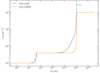 |
Fig. 3. Like Fig. 2, here we compare the density profiles for the J-type shock in mhd_vode, as well as the model presented in this paper. Good agreement is again observed, despite the lack of inflexion point recovery. |
Qualitatively comparing the T profiles in Fig. 2 we observe good agreement between the mhd_vode model and the UCLCHEM model’s computation of T in the shock-front described by Eq. (3). Both models reach approximately the same Tmax over an almost identical distance despite the UCLCHEM model beginning its heating prior to the mhd_vode model.
Further agreement is observed until d ≈ 1011 cm, whereby mhd_vode begins to cool rapidly, further exhibiting an inflexion point at d ≈ 1013 cm, causing T to drop from 5000 K to 300 K. As a result agreement diverges between 1011 < d < 1014 cm. This departure is a consequence of mhd_vode’s radiative cooling, which UCLCHEM does not implement.
Furthermore mhd_vode does not explicitly cool back to its initial temperature, though it does reach an equilibrium temperature very close to that of its initial temperature. Figure 2 shows the mhd_vode model cooling its gas to ≈10 K after d ≈ 1014 cm. The parameterised model presented here explicitly assumes that the gas cools back to Tinitial. In Fig. 2 this is 10 K.
Comparisons between nH models in Fig. 3 show qualitatively less agreement, especially regarding the peak nH. However, the UCLCHEM peak nH is within a factor of 2 of the mhd_vode model.
The inflexion point highlighted in Fig. 2 is also present within Fig. 3 at the same time. Similarly to before, we do not attempt to recover this feature. To assess the effect that this missing feature has on our approximation, and the subsequent chemistry that this model is used to inform, we directly compare the chemistry of H2O between mhd_vode and UCLCHEM. This is seen in Fig. 4. Importantly, the public version of mhd_vode used in this study does not include sputtering. Therefore for this comparison, we disable UCLCHEM’s sputtering treatment to compare chemistry with the same major gas-grain treatments present.
 |
Fig. 4. Evolution of H2O during the shock referenced in Figs. 2 and 3 in both mhd_vode and UCLCHEM. Within this figure, sputtering has been deactivated in UCLCHEM for the purposes of comparison. This implies that only gas-phase chemical reactions are active in these simulations so that the effect of the differences in the temperature profiles between mhd_vode and our approximation can be fairly evaluated. The abundance evolution of H2O up to d ≈ 1013 cm is in almost perfect agreement. This is in spite of the lack of inflexion point in both T and n between 1011 < d < 1014 cm. This proves that such a departure has negligible effect during the shock. mhd_vode manually cools H2O, hence the decrease in abundance at d ≈ 1014 cm. UCLCHEM does not implement this cooling. |
For the same initial conditions, mhd_vode and UCLCHEM produce the same H2O abundance behaviour despite UCLCHEM not recovering the observed inflexion point. This is true up to d = 1014 cm, where mhd_vode radiatively cools H2O, causing its abundance to drop sharply. UCLCHEM does not implement this form of cooling and so the H2O abundance does not drop sharply until a much greater distance into the shock.
Given that our model is never more than a factor of 3 away from the mhd_vode equivalent, and that the shocked H2O abundances are in almost perfect agreement, we consider our parameterisation of a J-type shock a good approximation of an equivalent shock model from an ideal-MHD simulation such as mhd_vode.
Part of our model is the simplifying assumption that the shock is steady-state. This is valid and physically justified as long as the cooling time of the shock is shorter than the time for which the shock velocity and the pre-shock conditions of the gas can change (Martinez 2009). In our grid runs, we switch back on grain chemistry and assume that the mantle ices instantaneously evaporate if the temperature of the gas T > 100 K. This is derived from plots within Fraser et al. (2001). We also assume that any species that have formed in the solid-state on the dust-grain will co-desorb alongside the mantle ices.
We note that the instantaneous evaporation of the ices in J-type shocks occurs before sputtering takes place. This is fully justified since this is the expected behaviour from the J-type shock’s rapid heating of gas and dust at the sharp shock front. For C-type shocks, we consider both processes, ice evaporation when T exceeds 100 K and sputtering. Since T is significantly lower in C-type shocks, evaporation is less efficient and so sputtering is more effective at releasing a fractional amount of the ices into the gas phase (see Jiménez-Serra et al. 2008, for details on the fractional sputtering technique implemented in UCLCHEM).
The qualitative agreement noted thus far between mhd_vode model and our parameterised model validates our steady-state assumption for the initial shock conditions applied here.
4.2. Identifying J-type shock behaviour
To identify unique J-type shock behaviour, we determine the average abundance across the post-shock region3 arising as a result of both J-type and C-type shocks for each model within our grid, and express the ratio of these two average abundances, χ(J)/χ(C). J-type shock enhanced molecules are therefore molecules that have χ(J)/χ(C) ≫ 1.
To assess the distribution of ratios across the entire grid we bin each model by its values of vs and nH and construct a 2D colour plot. The colour within each bin represents the ratio of the average post-shock abundances, χ(J)/χ(C), up to the dissipation length (or equivalent) for both shock types.
We also use the enhancement factor, fenhance, as a diagnostic. We define fenhance in Eq. (5).

χ(R) is the fractional abundance of the shocked molecule, whilst χ(0) is the fractional abundance of the molecule in a quiescent state. Within this study, we take χ(0) to be the abundance at simulation time t ≈ 0 years before any sputtering takes place. fenhance is therefore directly comparable to f in Table 1.
This analysis was performed for a range of different known shock-tracing molecules including CH3OH, H2O, SO, SO2 and HCN. We also investigated the behaviour of molecules such as SiO, however our analysis indicated that its behaviour was not noteworthy at the considered conditions. We attribute this to our shock velocities vs being too slow to efficiently sputter and form SiO.
4.2.1. CH3OH
Figure 5 shows the ratio of the average post-shock abundances up to the dissipation length (or equivalent) for each shock type. It is computed for C-type shock and J-type shock enhanced CH3OH for each model in the grid described in Table 2. Within this figure, χ(C) represents the average gas-phase abundance in a C-type shock achieved up to the dissipation length, whilst χ(J) is the average gas-phase abundance up to the cooling length for a J-type shock.
 |
Fig. 5. Ratio of the average J-type enhanced CH3OH abundance to the average C-type enhanced CH3OH abundance. As is clear, there is no chemical difference between J-type and C-type enhanced CH3OH, except at low vs and low nH. This major difference – a factor of 8000 – arises as a result of the C-type shock failing to sputter grain surface material whilst the J-type shock instantaneously evaporates grain surface CH3OH. |
Figure 5 shows that there is essentially no difference in chemistry between shock type for CH3OH, except the models where vs = 5 km s−1 and nH = 103 cm−3 as well as nH = 104 cm−3.
This unique disparity stems from the stark difference in gas-grain behaviour between shock types under these conditions. As Fig. 6 shows, the CH3OH abundance sharply increases as a result of instantaneous evaporation at d ≈ 107 cm in the J-type shock. In the C-type shock, neither evaporation nor sputtering occurs, meaning the CH3OH abundance remains relatively consistent throughout the shock.
This is confirmed in Figs. 6 and 7, which shows the CH3OH abundance as a function of distance through both C-type and J-type shocks with velocity vs = 5 km s−1 and density nH = 103 cm−3 and nH = 106 cm−3.
 |
Fig. 6. CH3OH abundances for a shock with initial velocity vs = 5 km s−1 and density nH = 103 cm−3. The shaded red region indicates the region beyond which the J-type shock has cooled to its equilibrium temperature. |
 |
Fig. 7. CH3OH abundances for a shock with initial velocity vs = 5 km s−1 and density nH = 106 cm−3. Again, the shaded red region indicates the region beyond which the J-type shock has cooled to its equilibrium temperature. |
At conditions excluding those already discussed, sputtering becomes efficient, hence the abundance ratios in Fig. 5 tending to 1 uniformly throughout the rest of the grid as a result of CH3OH being co-desorbed in a J-type shock and sputtered in a C-type shock in equal measure. Importantly, following injection/sputtering there is minimal subsequent gas-phase chemistry in either shock, hence reinforcing the common abundances achieved in Fig. 5 regardless of shock type.
As a result of the J-type shock’s rapid heating, instantaneous evaporation occurs well before any sputtering activity in a C-type shock. In both shocks, the same amount of CH3OH is released from the dust-grains owing to self-consistent initial conditions from phase 1 of UCLCHEM.
4.2.2. H2O
The abundance ratios for H2O is shown in Fig. 8. Much like CH3OH in Sect. 4.2.1, H2O behaves similarly at vs = 5 km s−1 and nH = 103 cm−3 as well as nH = 104 cm−3 owing to the same processes; in other words the J-type shock instantaneously evaporates material whilst the C-type shock neither sputters nor evaporates.
 |
Fig. 8. Ratio of the average J-type enhanced H2O abundance to the average C-type enhanced H2O abundance. The largest difference between average shock type abundance is at vs = 5 km s−1 and nH = 103 cm−3 and nH = 104 cm−3 where the ratio exceeds 1000. |
Outside of this, the biggest difference between C-type and J-type shocks peaks at vs < 10 km s−1 and nH = 103 cm−3. The enhancement factors drop off to ≈1 at velocities and densities greater than these.
Figures 9 and 10 shows the H2O abundances as a function of distance through the shock for C-type and J-type shocks with velocity vs = 5 km s−1 and density nH = 103 and nH = 106 cm−3.
 |
Fig. 9. H2O abundances for a shock with initial velocity vs = 5 km s−1 and density nH = 103 cm−3. |
 |
Fig. 10. H2O abundances for a shock with initial velocity vs = 5 km s−1 and density nH = 106 cm−3. |
In the J-type shock profiles from Figs. 9 and 10, the gas phase abundance of H2O increases sharply at ≈107 cm. This feature arises as a result of evaporation of the solid state material frozen on to the dust grains, e.g. the ices. The C-type shock may also undergo an increase in gas phase H2O at a later time in the shock as a result of sputtering, providing that the initial shock conditions enable the sputtering process. In our models, sputtering does not occur at vs = 5 km s−1 and nH = 103 cm−3 as well as nH = 104 cm−3, hence the large difference in average abundance at these models in Fig. 8.
Post-evaporation features within Figs. 9 and 10 begin to explain the more minor gas-phase enhancement in Fig. 8. For the J-type shock in Fig. 9, the abundance of H2O increases to a maximum of ≈3 × 10⁻⁴, approximately 6 times the post-evaporation abundance, at around d ≈ 1013 cm. This effect is largest at nH = 103 cm−3 and is present as nH increases, though the magnitude of the gas-phase enhancement does decrease as nH increases. At nH = 106 cm−3 (Fig. 10) there is no post-evaporation gas phase abundance change in H2O, thus eliminating the effect altogether.
Investigating the C-type shock in Figs. 9 and 10, we observe no post-sputtering increase in H2O, regardless of nH. This, coupled with the decreasing gas-phase enhancement in the J-type as nH increases, results in both shock types tending to the same abundance.
This explains why the largest enhancement is seen at low vs, low nH. As nH increases, an overall decrease in the post-injection gas phase abundance change is observed, despite the evaporated H2O increasing with nH. As vs increases, the peak temperature of the shock also rises, allowing gas-phase H2O to be destroyed. For a J-type shock, H2O destruction begins at vs = 11 km s−1 when Tmax > 6000 K.
4.2.3. SO
Figure 11 shows the average abundance ratios for SO. Interestingly, Fig. 11 shows that SO is not produced more efficiently in a J-type shock than a C-type shock in our parameter space. In actuality, for nH > 104 cm−3 the ratio χ(J)/χ(C) ≈ 1, indicating that at high density both shocks are able to enhance SO to similar degrees.
 |
Fig. 11. Ratio of the average J-type enhanced SO abundance to the average C-type enhanced SO abundance. The largest difference between peak shock type abundance is at nH = 103 cm−3. The shock conditions that produce unique chemistry in this parameter space are those with nH < 105 cm−3. |
The behaviour of SO at nH < 104 cm−3 is starkly different. Considering the n = 103 cm−3 row within Fig. 11, it can be observed that the peak ratio of ≈10 occurs at vs = 5 km s−1. To explain such behaviour, consider the SO abundance as a function of distance in Figs. 12 and 13 for a shock of vs = 5 km s−1 with density from nH = 103 cm−3 and nH = 106 cm−3.
 |
Fig. 12. SO abundances for a shock with initial velocity vs = 5 km s−1 and density nH = 103 cm−3. |
 |
Fig. 13. SO abundances for a shock with initial velocity vs = 5 km s−1 and density nH = 106 cm−3. |
Comparing the vs = 5 km s−1 and nH = 103 cm−3 model in Fig. 11 with the abundance profile for the same initial conditions in Fig. 12 begins to explain the peak abundance ratio. It is clear that this arises as a result of the J-type shock injecting SO from the grain surface, whilst the C-type shock cannot sputter at these conditions. As d approaches 1013 cm the SO abundance peaks at around 10−7 – an enhancement relative to the initial SO abundance of ≈100. However, towards d ≈ 1013 cm the SO abundance drops off sharply as SO is destroyed. This destruction skews the average SO abundance, hence the peak abundance ratio in Fig. 11 being far smaller than the peak enhancement of 100. Moreover, Tmax of a C-type shock of vs = 5 km s−1 is 85 K. Such a minimal change in T through the shock is not sufficient to drive any significant gas-phase chemistry, hence the SO abundance remaining relatively constant throughout the shock in Fig. 12.
Additionally, as vs increases the C-type shock sputtering becomes more effective whilst the J-type shock destroys SO at high T, resulting in the average post-shock abundance in a J-type shock being less than the equivalent C-type shock. For example at vs = 15 km s−1 and nH = 103 cm−3, the J-type shock average abundance is 3 × 10⁻² times smaller than the C-type shock equivalent.
This is true of the models at nH = 104 cm−3 as well, though here we note that the C-type shock sputtering is more efficient therefore exacerbating the differences between average abundance in shock type. Evident here is the J-type shock abundance at vs = 15 km s−1 and nH = 104 cm−3 being 1 × 10⁻² times smaller than C-type shock equivalent.
Figures 12 and 13 also shows that as nH increases, the abundances at large d between shock types behaves universally and tends to a similar limit indicating that the dominant destruction mechanism becomes a density limited process. This therefore means that at lower nH, the enhancement is governed by a combination of gas-phase and dust-grain chemistry, whilst at large values of nH the enhancement factor is governed by dust-grain chemistry alone.
4.3. SO2
Figure 14 shows the abundance ratios for SO2. Evident when considering Fig. 14 is the similarity between it and the SO behaviour in Fig. 11. Given that SO2 can form via SO dependent reactions such as O + SO → SO2, the similarity in behaviour is not surprising.
 |
Fig. 14. Ratio of the maximum J-type enhanced SO2 abundance to the maximum C-type enhanced SO2 abundance. The largest difference between peak shock type abundance is at nH = 103 cm−3 much like the SO abundance in Fig. 11. |
Figure 14 shows largely the same trends as Fig. 11 did. For instance, we see the same behaviour in χ(J)/χ(C) ≈ 1 at nH > 104 cm−3 in Fig. 11, along with the same model having the same abundance ratio in Fig. 11. Curiously, this peak abundance ratio is ≈200, whilst in Fig. 11 it was ≈10. These global trends and behaviour are expected given the close chemical relationship between SO and SO2.
Figures 15 and 16 shows the SO2 abundances as a function of distance for both C-type and J-type shocks at v = 5 km s−1 through nH = 103 cm−3 and nH = 106 cm−3. Much like SO in Figs. 12 and 13, both C-type and J-type shock abundance tend to the same value as nH increases. Furthermore the same behaviour is seen at low nH. This implies that any changes to SO in a shock should be mirrored – at least in terms of qualitative behaviour – by SO2 as well.
 |
Fig. 15. SO2 abundances for a shock with initial velocity vs = 5 km s−1 and density of nH = 103 cm−3. |
 |
Fig. 16. SO2 abundances for a shock with initial velocity vs = 5 km s−1 and density of nH = 106 cm−3. |
4.4. HCN
As Fig. 17 shows, the peak abundance ratio occurs at vs < 9 km s−1 and nH = 103 cm−3, with the degree of this ratio decreasing as vs increases. As discussed before in Sects. 4.2.1–4.2.3 and 4.3, it is the stark differences in sputtering and evaporation behaviour between shock types at these conditions that gives rise to this feature.
 |
Fig. 17. Ratio of the average J-type enhanced HCN abundance to the average C-type enhanced HCN abundance. The largest difference between peak shock type abundance is at vs < 9 km s−1 and nH = 103 cm−3. High vs, low nH shocks show C-type shocks are more efficient enhancers of HCN than equivalent J-type shocks. |
Much like SO and SO2 beforehand, the ratio for nH > 104 cm−3 of Fig. 17 shows very little departure from 1 indicating that both shock types enhance HCN to the same or similar degree. Again similarly to SO and SO2 the enhancements at vs = 12−15 km s−1 and nH = 103 − 104 cm−3 indicate C-type shocks are more effective enhancers of HCN than a J-type shock. As Table 2 shows, J-type shocks have far higher Tmax than an equivalent C-type shock. This implies that between vs = 12−15 km s−1 J-type shocks are capable of destroying HCN whilst an equivalent C-type shock cannot reach a similarly high T, therefore allowing HCN to continue formation or not undergo destruction at all.
Individual abundance profiles for HCN are shown in Figs. 18 and 19. As is consistent with other figures, the immediate post-evaporation abundance increases as nH. Despite this, the maximal post-shock gas-phase enhancement of HCN is at lower density, with the effect dropping off as nH increases.
 |
Fig. 18. HCN abundances for a shock with initial velocity vs = 5 km s−1 and density of nH = 103 cm−3. |
 |
Fig. 19. HCN abundances for a shock with initial velocity vs = 5 km s−1 and density of nH = 106 cm−3. |
Much like previous figures, Fig. 18 explains why the J-type shock HCN abundance is so much greater than the C-type shock HCN abundance. Similarly to before, C-type shock sputtering is not possible at vs = 5 km s−1 and nH = 103 cm−3 whilst the J-type shock is capable of instantaneously evaporating the grain-mantle material. Unlike previous molecules however, this behaviour continues up to vs = 12 km s−1. As nH increases to nH = 106 cm−3 sputtering becomes more efficient and the post-evaporation abundance increases no longer occur. Both of these factors combined allows the HCN abundance in both shock types to tend to the same limit of ≈5 × 10⁻⁸. As shown by Fig. 17, this behaviour occurs at all values of vs for nH = 105 cm−3 and nH = 106 cm−3.
5. The shocks in L1157-B2
Vasta et al. (2012) observed H2O lines towards the B1 and B2 knots of L1157. In conjunction with theoretical shock models, they theorise that J-type shocks could be a prominent source of this emission. Consequently, having thus far found several unique J-type shock chemical distinctions, specifically with respect to H2O and HCN, we qualitatively apply the results from our grid of models to the B2 region of L1157 in an effort to further categorise the type of shock responsible for its emission. We also compare the results to the measured abundances and enhancement factors in Table 1 to further constrain the shock type. Crucially, as mentioned in Sect. 2.2, the measured abundances are likely subject to large uncertainties owing to the optically thin and thermalised line assumptions required to determine them.
We focus on B2 and not B1 for a number of reasons. Firstly, Gusdorf et al. (2008) theorised that B1 is the result of a combination of C-type and J-type shocks, especially in regards to the SiO and H2 observations. This implies that B2 is also likely to be related to J-type shocks in some form. Further studies such as those by Vasta et al. (2012) also conclude that B2 likely hosts a J-type shock, either singularly or in combination with a C-type shock component. Lastly, given the low and high angular resolution observations of the B2 region by Benedettini et al. (2007, 2013), it seems that B2 is much more homogeneous than B1. This homogeneity removes any influence of successive shock driven chemistry, making B2 the ideal laboratory with which to test this type of shock diagnostic methodology.
5.1. CH3OH
We showed in Sect. 4.2.1 that CH3OH undergoes no enhancement after its initial release from the dust grains into the gas-phase. This therefore implies that f(B1) and f(B2) in Table 1 are dependent only upon the sputtered abundance and not the gas phase chemistry CH3OH undergoes.
According to Bachiller & Pérez Gutiérrez (1997) L1157-B2 has a CH3OH abundance of ≈2.2 × 10⁻⁵. CH3OH’s minimal gas-phase chemistry therefore means that shock enhancing CH3OH to this abundance is solely a result of sputtering and/or evaporation, which itself is a density-dependent effect. This implies that shock enhanced CH3OH traces the amount of CH3OH on the grains and therefore the density of the pre-shocked region, rather than the shock velocity.
According to Table 1 L1157-B2 has a CH3OH abundance 500 times larger than the central protostar, L1157-mm, where the χCH3OH = 4.5 × 10⁻⁸. This is consistent with either a C-type of J-type shock impacting a region of pre-shock density n = 103 cm−3. This pre-shock density also produces a pre-shock abundance χCH3OH ≈ 2 × 10⁻⁹, approximately consistent with the pre-shock density measured towards L1157-mm. Importantly this is also consistent with the pre-shock density reported by Gómez-Ruiz et al. (2016) towards L1157-B2. It remains difficult, however, to use CH3OH as a tracer of either shock type or shock velocity owing to its consistent gas-phase chemistry under differing physical conditions.
5.2. H2O
We showed in Sect. 4.2.2 that H2O can trace J-type shocks at vs < 10 km s−1 and nH = 103 cm−3.
In application to L1157-B2, however, no enhancement ratio was determined by Vasta et al. (2012). The H2O abundance towards L1157-B2 was determined as 1 × 10⁻⁶. This abundance is smaller than all of the immediate post-evaporation/post-sputtering abundances that our models show. These models can, however, recover an abundance similar to this for a shock of vs < 10 km s−1 and nH = 103 cm−3. Matching the exact measured abundance is only achievable during the post-evaporation H2O abundance changes. At vs > 10 km s−1, H2O is destroyed in the gas-phase allowing the abundance to drop the order of 10−6, though as the temperature increases beyond that achieved in vs ≈ 12 km s−1 the abundance falls well below 10−6.
Importantly, the best matching shock conditions are also consistent with those determined by Gómez-Ruiz et al. (2016) as vs ≈ 10 km s−1 and nH ≈ 103 cm−3. However, as we do not vary the freeze-out efficiency in this study we cannot conclude with certainty whether the observed abundance is solely a result of the shock or a combination of varying freeze-out efficiency and shock action. A lower freeze-out efficiency and slower shock velocity could reproduce a similar abundance to the observed abundance.
5.3. HCN
We showed in Sect. 4.4 that HCN can undergo unique J-type shock enhancement at low vs and low nH. As vs and nH increase the abundances in each shock type tend to a similar value, implying that HCN can trace low vs and low nH J-type shocks only.
Bachiller & Pérez Gutiérrez (1997) estimate the HCN abundance towards L1157-B2 as 5.5 × 10⁻⁷, undergoing an enhancement by a factor of ≈150 relative to the L1157-mm HCN abundance of 3.6 × 10⁻⁹. Figures 18 and 19 shows both C-type and J-type shocks are capable of enhancing HCN to the same degree at high nH. Figures 18 and 19 also shows that whilst our models do not recover the exact initial HCN abundance of 3.6 × 10⁻⁹ as measured towards L1157-mm, they are capable of re-producing a value of ≈10−9 in the range nH = 103 − 105 cm−3.
Considering the enhancement factor of 150, Fig. 17 shows that this is only possible in a J-type shock between vs = 6−8 km s−1 and nH = 103 cm−3, which is approximately consistent with the shock parameters determined by Gómez-Ruiz et al. (2016).
5.4. SO
Bachiller & Pérez Gutiérrez (1997) report that L1157-B2 is more abundant in SO than SO2. Crucially, the ranges defined for SO abundance in L1157-B1 and L1157-B2 by Bachiller & Pérez Gutiérrez (1997) intersect, likely because of the close chemical relationship between SO and SO2.
The initial SO abundance measured towards L1157-mm is 5.0 × 10⁻⁹. Much like HCN, our models are capable of recovering an initial SO abundance of ≈10−9 in the range nH = 103 − 105 cm−3.
Bachiller & Pérez Gutiérrez (1997) measure the abundance of SO towards L1157-B2 as 2.0−5.0 × 10⁻⁷, which yields an enhancement ratio of 60−100. Our models, as is evident from Fig. 11, show that on average a J-type shock is not able to enhance SO to the same degree that an equivalent C-type can produce if both shock types can sputter and/or inject ice material into the gas-phase. This, therefore, implies that any unique SO enhancement is the result of a C-type shock.
5.5. SO2
According to Table 1, L1157-B2 is subject to an SO2 enhancement of ≈20 with an initial abundance of 3.0 × 10⁻⁸. None of the models produced here are capable of reproducing an initial abundance of this order. This indicates that SO2 has formed more efficiently towards L1157 than our models would indicate. In actuality, Table 1 shows SO2 being initially more abundant than SO by almost an order of magnitude.
Furthermore, the relative similarities in global behaviour between SO and SO2 mean the same conclusion applies here, i.e. within the grid of models, C-type shocks are the producers of unique SO2 behaviour rather than J-type shocks.
6. Discussion
It is clear from Sect. 4 that the CH3OH, H2O and HCN abundances do allude to a shock component within L1157-B2 of vs = 8−11 km s−1 impacting a region of pre-shock density of nH = 103 cm−3. However, CH3OH does not undergo any gas-phase enhancement unique to a specific shock type, rendering it a reliable tracer of pre-shock density in the majority of cases.
According to Figs. 6 and 7, CH3OH undergoes no post-evaporation gas-phase abundance change. Recent evidence (Holdship et al. 2019, and references therein) indicates that contrary to this finding, CH3OH is destroyed in highly energetic, high-temperature events such as shocks. The lack of CH3OH destruction in our models could indicate that the network used, in this instance UMIST, may be missing some of the dominant high-temperature destruction routes for CH3OH. Alternatively, such findings could point to observations capturing a form of progressive erosion of CH3OH from the grain surfaces as first proposed by Jiménez-Serra et al. (2005). Nevertheless, there is sufficient evidence to consider the CH3OH abundances determined here as upper limits.
To address the apparent lack of destruction we performed a test whereby we included several combustion literature derived CH3OH destruction routes via collisional dissociation with H in our network. We selected these reactions as they are thought to be the most efficient mechanism for CH3OH destruction in dissociative J-type shocks (Suutarinen et al. 2014). Specifically, the reactions included are CH3OH + H → CH3 + H2O (Hidaka et al. 1989), CH3OH + H → H2 + CH2OH (Li & Williams 1996) and CH3OH + H → H2 + CH3O (Warnatz 2012). However, the addition of these reactions produced complete destruction of gas-phase CH3OH at high temperature. This may be because the destruction reactions we included have only been measured under combustion conditions and hence are not necessarily accurate for the densities and temperatures of the ISM environments of our study (Balucani, priv. comm.). We therefore cannot draw any definitive conclusions regarding CH3OH abundance as a tracer of shock type, beyond the upper-limits derived here, until a follow-up study is performed to investigate the prominent reactions responsible for CH3OH’s high-temperature destruction. However, the injection behaviour of CH3OH provides an excellent tracer of pre-shock density.
H2O and HCN both exhibit degrees of enhancement that peak at a factor of 60 relative to a C-type shock at low vs low nH. However the behaviour of both HCN and H2O at larger nH tends to a common trend between both shock types. Such behaviour indicates that using H2O and HCN as shock type tracers is only valid, and likely only accurate, at lower values of vs and nH.
Importantly we do not deplete the initial abundance of S. As Jenkins (2009) highlight, the observed abundance of S+ in early-star forming regions matches the approximate cosmic abundance. However, as noted by Laas & Caselli (2019), the abundance of S-bearing species in molecular clouds is reduced significantly, hence the term “depletion”. Astrochemical models therefore tend to reduce the elemental S abundance to 1% of its cosmic abundance in order to ensure that the S-bearing molecular inventory is representative of the region studied, for example a molecular cloud. Given the uncertainty surrounding the exact depletion factors, both universally as well as locally, to introduce a depletion factor here would introduce another degree of freedom and another potentially significant source of error that may potentially yield a larger disagreement between the predictions and observations. We therefore fix our initial S abundance as solar.
Studies such as those by Benedettini et al. (2007) have shown the B1 and B2 knots themselves have sub-structure. These sub-structural features are likely not thermalised with their surroundings, rendering the observed molecular abundances more abundant than one discrete shock event would produce. It is also possible that B2 may host multiple velocity components, meaning that different molecules may trace different components of the shock. However, the upper limits of the CH3OH abundance for L1157-B2 derived here are consistent with a shock of pre-shock density nH = 103 cm−3 which matches the pre-shock density determined by Gómez-Ruiz et al. (2016).
Gómez-Ruiz et al. (2016) use NH3 and H2O observations to derive their estimates of the shock parameters. Our H2O abundance trends show an immediate post-shock enhanced abundance of between 10−4 and 10−5, around a factor 10 to 102 higher than Vasta et al. (2012) would indicate. As mentioned previously, some models are capable of achieving an H2O abundance approximately consistent with observations providing that the shock is capable of dissociating H2O. Consequently, the observations could be tracing this dissociated H2O component. Alternatively, our simulations may over-estimate the formation efficiency of H2O on the grains, thus allowing more H2O to be released from the grains in sputtering or evaporation than is realistic.
From Table 1 the abundance of H2O in L1157 is around 2 orders of magnitude higher in B1 than B2, indicating that gas-phase H2O has either been destroyed in L1157-B2 or that it has had sufficient time to freeze on to the surface of the dust.
The behaviour of SO and SO2 in Figs. 11 and 14 show that they both reliably trace low vs, low nH C-type shocks. We have thus far established that L1157-B2 bears some signatures of J-type shock chemistry, but SO and SO2 trace predominantly C-type shocks in the parameter space considered. However, the SO and SO2 behaviour, coupled with the SO and SO2 enhancements in L1157-B2, would seemingly imply that L1157-B2 is host to either a C-type shock component as well as a J-type shock component or a singular component being mixed-type in nature. This mixed-type shock could potentially be a J-type shock that is evolving to take on a more C-type shock structure. Both of these scenarios are consistent with the observed trends. However, to confirm either scenario would require a more detailed model of a mixed-type shock, though observations such as those by Benedettini et al. (2007, 2013) are sufficient to continue exploring this question.
Further observational constraints will surely also be provided by SOLIS (Ceccarelli et al. 2017). Such data may allow classification of whether B2 hosts any sub-structure, in turn informing even further constraints on theoretical models of shock action.
7. Summary
We have developed a parameterised model of an isothermal, planar J-type shock wave as a module to the astrochemical code UCLCHEM. We compute a grid of models across the parameter space vs = 5−15 km s−1 and nH = 103 − 106 cm−3 using our J-type shock model as well as the pre-existing C-type module to quantify the different chemical abundance trends in each shock type. We find the following.
-
1.
Our results show that whilst a theoretical distinction in J-type shock chemistry is found in molecules such as H2O and HCN, it is largely unique to low vs, low nH shocks owing to the extreme temperatures J-type shocks are capable of reaching at high values of vs. Furthermore, the largest differences in chemistry between shock types arises as a result of the different sputtering and evaporation behaviours between shock types at low vs and low nH.
-
2.
We find that CH3OH is enhanced by shocks and is a reliable probe of the pre-shock gas density, however we find no difference between its gas-phase abundance between shock type. Recent evidence (Holdship et al. 2019) indicates that CH3OH is destroyed in high T shocks, indicating that chemical networks lack the high T reactions that permit CH3OH to be destroyed. Consequently, astrochemical simulations such as the one presented here can only provide upper limits of the shock-enhanced CH3OH abundance.
-
3.
Finally in our application to the L1157-B2 region, we find that fractional abundances are consistent with both C-type and J-type shock emission, potentially indicating the prevalence a mixed-type shock or multiple shock components. Crucially, however, the similarities in abundances at the initial conditions considered here indicate that the dominant factors affecting shock chemistry are more dependent on the initial shock conditions and not the shock type.
Acknowledgments
T. A. J. is funded by an STFC studentship, and thanks the STFC accordingly. I. J.-S. has received partial support from the Spanish FEDER (project number ESP2017-86582-C4-1-R), and State Research Agency (AEI) through project number MDM-2017-0737 Unidad de Excelencia “María de Maeztu” – Centro de Astrobiología (INTA-CSIC). The authors would like to thank the anonymous referee for their very valuable comments that helped improve the manuscript. We also thank D. Williams, R. Garrod, and N. Balucani for their discussions and opinions on aspects of this paper.
References
- Allen, M., & Robinson, G. W. 1977, AJ, 212, 396 [NASA ADS] [CrossRef] [Google Scholar]
- Bachiller, R., & Pérez Gutiérrez, M. 1997, ApJ, 487, L93 [NASA ADS] [CrossRef] [Google Scholar]
- Bachiller, R., Perez-Gutierrez, M., Kumar, M. S. N., & Tafalla, M. 2001, A&A, 372, 899 [NASA ADS] [CrossRef] [EDP Sciences] [Google Scholar]
- Baulch, D. L., Pilling, M. J., Cobos, C. J., et al. 1992, J. Phys. Chem. Ref. Data, 21, 411 [NASA ADS] [CrossRef] [Google Scholar]
- Benedettini, M., Viti, S., Codella, C., et al. 2007, MNRAS, 381, 1127 [NASA ADS] [CrossRef] [Google Scholar]
- Benedettini, M., Busquet, G., Lefloch, B., et al. 2012, A&A, 539, L3 [NASA ADS] [CrossRef] [EDP Sciences] [Google Scholar]
- Benedettini, M., Viti, S., Codella, C., et al. 2013, MNRAS, 436, 179 [NASA ADS] [CrossRef] [Google Scholar]
- Ceccarelli, C., Caselli, P., Fontani, F., et al. 2017, ApJ, 850, 176 [NASA ADS] [CrossRef] [Google Scholar]
- Charnley, S. B. 1997, ApJ, 481, 396 [NASA ADS] [CrossRef] [Google Scholar]
- Chièze, J. P., Des ForÉTs, G. P., & Flower, D. R. 1998, MNRAS, 295, 672 [NASA ADS] [CrossRef] [Google Scholar]
- Draine, B. T. 1980, ApJ, 241, 1021 [NASA ADS] [CrossRef] [Google Scholar]
- Draine, B. T., Roberge, W. G., & Dalgarno, A. 1983, ApJ, 264, 485 [NASA ADS] [CrossRef] [Google Scholar]
- Flower, D. R., & Des ForÉTs, G. P. 2015, A&A, 578, A63 [NASA ADS] [CrossRef] [EDP Sciences] [Google Scholar]
- Flower, D. R., Le Bourlot, J., Des ForÉTs, G. P., & Cabrit, S. 2003a, Space Sci., 287, 183 [NASA ADS] [CrossRef] [Google Scholar]
- Flower, D. R., Bourlot, J. L., Des ForÉTs, G. P., & Cabrit, S. 2003b, MNRAS, 80, 70 [NASA ADS] [CrossRef] [Google Scholar]
- Fraser, H. J., Collings, M. P., McCoustra, M. R., & Williams, D. A. 2001, MNRAS, 327, 1165 [NASA ADS] [CrossRef] [Google Scholar]
- Fuchs, G. W., Cuppen, H. M., Ioppolo, S., et al. 2009, A&A, 505, 629 [NASA ADS] [CrossRef] [EDP Sciences] [Google Scholar]
- Garrod, R. T., Weaver, S. L. W., & Herbst, E. 2008, ApJ, 682, 283 [NASA ADS] [CrossRef] [Google Scholar]
- Gidalevich, E. Y. 1966, Astrofizika, 02, 1966 [Google Scholar]
- Godard, B., Des ForÉTs, G. P., Lesaffre, P., et al. 2019, A&A, 622, A208 [NASA ADS] [CrossRef] [EDP Sciences] [Google Scholar]
- Gómez-Ruiz, A. I., Codella, C., Viti, S., et al. 2016, MNRAS, 462, 2203 [NASA ADS] [CrossRef] [Google Scholar]
- Gueth, F., Guilloteau, S., & Bachiller, R. 1996, A&A, 307, 891 [NASA ADS] [Google Scholar]
- Gusdorf, A., Des ForÉTs, G. P., Cabrit, S., & Flower, D. R. 2008, A&A, 490, 695 [NASA ADS] [CrossRef] [EDP Sciences] [Google Scholar]
- Hidaka, Y., Oki, T., Kawano, H., & Higashihara, T. 1989, J. Phys. Chem., 93, 7134 [CrossRef] [Google Scholar]
- Holdship, J., Viti, S., Jiménez-Serra, I., Makrymallis, A., & Priestley, F. 2017, AJ, 154, 38 [NASA ADS] [CrossRef] [Google Scholar]
- Holdship, J., Viti, S., Codella, C., et al. 2019, AJ, 880, 138 [CrossRef] [Google Scholar]
- Hollenbach, D., & McKee, C. F. 1989, ApJ, 342, 306 [NASA ADS] [CrossRef] [Google Scholar]
- Hugoniot, H. 1889, J. l’Ecole Polytech., 58, 1 [Google Scholar]
- Jenkins, E. B. 2009, ApJ, 700, 1299 [NASA ADS] [CrossRef] [Google Scholar]
- Jiménez-Serra, I., Caselli, P., Martin-Pintado, J., & Hartquist, T. W. 2008, A&A, 482, 549 [NASA ADS] [CrossRef] [EDP Sciences] [Google Scholar]
- Jiménez-Serra, I., Martín-Pintado, J., Rodríguez-Franco, A., & Martín, S. 2005, ApJ, 627, L121 [NASA ADS] [CrossRef] [Google Scholar]
- Jiménez-Serra, I., Caselli, P., Martín-Pintado, J., & Hartquist, T. W. 2008, A&A, 482, 549 [NASA ADS] [CrossRef] [EDP Sciences] [Google Scholar]
- Laas, J. C., & Caselli, P. 2019, A&A, 624, A108 [CrossRef] [EDP Sciences] [Google Scholar]
- Lefloch, B., Cabrit, S., Codella, C., et al. 2010, A&A, 518, L113 [NASA ADS] [CrossRef] [EDP Sciences] [Google Scholar]
- Lefloch, B., Bachiller, R., Ceccarelli, C., et al. 2018, MNRAS, 477, 4792 [NASA ADS] [CrossRef] [Google Scholar]
- Li, S. C., & Williams, F. A. 1996, Symp. (Int.) Combust., 26, 1017 [CrossRef] [Google Scholar]
- Looney, L. W., Tobin, J. J., & Kwon, W. 2007, ApJ, 670, L131 [NASA ADS] [CrossRef] [Google Scholar]
- Martinez, A. P. 2009, Astron. J., 2, 1 [NASA ADS] [CrossRef] [Google Scholar]
- McElroy, D., Walsh, C., Markwick, A. J., et al. 2013, A&A, 550, A36 [NASA ADS] [CrossRef] [EDP Sciences] [Google Scholar]
- Podio, L., Codella, C., Gueth, F., et al. 2016, A&A, 593, L4 [NASA ADS] [CrossRef] [EDP Sciences] [Google Scholar]
- Rankine, W. J. M. 1870, Philos. Trans. R. Soc. London, 160, 277 [NASA ADS] [CrossRef] [Google Scholar]
- Rawlings, J. M. C., Hartquist, T. W., Menten, K. M., & Williams, D. A. 1992, MNRAS, 255, 471 [NASA ADS] [CrossRef] [Google Scholar]
- Rodríguez-Fernández, N. J., Tafalla, M., Gueth, F., & Bachiller, R. 2010, A&A, 516, A98 [NASA ADS] [CrossRef] [EDP Sciences] [Google Scholar]
- Shu, F. H., Ruden, S. P., Lada, C. J., & Lizano, S. 1991, ApJ, 370, L31 [NASA ADS] [CrossRef] [Google Scholar]
- Snell, R. L., Loren, R. B., & Plambeck, R. L. 1980, ApJ, 239, L17 [NASA ADS] [CrossRef] [Google Scholar]
- Suutarinen, A. N., Kristensen, L. E., Mottram, J. C., Fraser, H. J., & Van Dishoeck, E. F. 2014, MNRAS, 440, 1844 [NASA ADS] [CrossRef] [Google Scholar]
- Tafalla, M., & Bachiller, R. 1995, ApJ, 443, L37 [Google Scholar]
- Tielens, A. G. G. M., & Whittet, D. C. B. 1997, Molecules in Astrophysics: Probes & Processes: Abstract Book, 178, 45 [NASA ADS] [Google Scholar]
- Umemoto, T., Iwata, T., Fukui, Y., et al. 1992, ApJ, 392, L83 [NASA ADS] [CrossRef] [Google Scholar]
- van Dishoeck, E. F., Kristensen, L. E., Benz, A. O., et al. 2010, PASP, 123, 138 [Google Scholar]
- van Dishoeck, E. F., Herbst, E., & Neufeld, D. A. 2013, Chem. Rev., 113, 9043 [NASA ADS] [CrossRef] [PubMed] [Google Scholar]
- Vasta, M., Codella, C., Lorenzani, A., et al. 2012, A&A, 537, A98 [NASA ADS] [CrossRef] [EDP Sciences] [Google Scholar]
- Viti, S., Jiménez-Serra, I., Yates, J. A., et al. 2011, ApJ, 740, L3 [NASA ADS] [CrossRef] [Google Scholar]
- Warnatz, J. 2012, Combustion Chemistry (New York: Springer), 197 [Google Scholar]
- Williams, D. A., & Viti, S. 2013, Observational Molecular Astronomy (Cambridge: Cambridge University Press) [CrossRef] [Google Scholar]
- Zel’dovich, Y. B., & Raizer, Y. P. 1967, Physics of Shock Waves and High-temperature Hydrodynamic Phenomena (New York: Academic Press) [Google Scholar]
- Zhang, Q., & Zheng, X. 1997, ApJ, 474, L719 [NASA ADS] [CrossRef] [Google Scholar]
All Tables
Abundances χ of known shock enhanced molecules and their enhancement factors f (relative to χ(0)) in the two L1157 knots B1 and B2.
All Figures
|
Fig. 1. Spitzer/IRAC 8 μm image of the L1157 outflow. (Podio et al. 2016). Shown as black squares are the shock events B0, B1 and B2. The class-0 protostar L1157-mm that drives the outflow is also labelled. The black line overplotted is the precession model thought to be responsible for the creation of the observed knots. As is visible here, B2 is far less intense in emission than B0/B1. |
| In the text | |
|
Fig. 2. Comparing the temperature structure of a J-type shock with v = 10 km s−1 and nH = 103 cm−3 computed with the model presented in this paper and the mhd_vode model by Flower & Des ForÉts (2015). Good agreement is observed, despite our approximation not recovering all of the features in the mhd_vode profile. The model built for UCLCHEM is also isothermal such that it cools back to its initial temperature, whereas mhd_vode is not despite it cooling to ≈10 K in this instance. |
| In the text | |
|
Fig. 3. Like Fig. 2, here we compare the density profiles for the J-type shock in mhd_vode, as well as the model presented in this paper. Good agreement is again observed, despite the lack of inflexion point recovery. |
| In the text | |
|
Fig. 4. Evolution of H2O during the shock referenced in Figs. 2 and 3 in both mhd_vode and UCLCHEM. Within this figure, sputtering has been deactivated in UCLCHEM for the purposes of comparison. This implies that only gas-phase chemical reactions are active in these simulations so that the effect of the differences in the temperature profiles between mhd_vode and our approximation can be fairly evaluated. The abundance evolution of H2O up to d ≈ 1013 cm is in almost perfect agreement. This is in spite of the lack of inflexion point in both T and n between 1011 < d < 1014 cm. This proves that such a departure has negligible effect during the shock. mhd_vode manually cools H2O, hence the decrease in abundance at d ≈ 1014 cm. UCLCHEM does not implement this cooling. |
| In the text | |
|
Fig. 5. Ratio of the average J-type enhanced CH3OH abundance to the average C-type enhanced CH3OH abundance. As is clear, there is no chemical difference between J-type and C-type enhanced CH3OH, except at low vs and low nH. This major difference – a factor of 8000 – arises as a result of the C-type shock failing to sputter grain surface material whilst the J-type shock instantaneously evaporates grain surface CH3OH. |
| In the text | |
|
Fig. 6. CH3OH abundances for a shock with initial velocity vs = 5 km s−1 and density nH = 103 cm−3. The shaded red region indicates the region beyond which the J-type shock has cooled to its equilibrium temperature. |
| In the text | |
|
Fig. 7. CH3OH abundances for a shock with initial velocity vs = 5 km s−1 and density nH = 106 cm−3. Again, the shaded red region indicates the region beyond which the J-type shock has cooled to its equilibrium temperature. |
| In the text | |
|
Fig. 8. Ratio of the average J-type enhanced H2O abundance to the average C-type enhanced H2O abundance. The largest difference between average shock type abundance is at vs = 5 km s−1 and nH = 103 cm−3 and nH = 104 cm−3 where the ratio exceeds 1000. |
| In the text | |
|
Fig. 9. H2O abundances for a shock with initial velocity vs = 5 km s−1 and density nH = 103 cm−3. |
| In the text | |
|
Fig. 10. H2O abundances for a shock with initial velocity vs = 5 km s−1 and density nH = 106 cm−3. |
| In the text | |
|
Fig. 11. Ratio of the average J-type enhanced SO abundance to the average C-type enhanced SO abundance. The largest difference between peak shock type abundance is at nH = 103 cm−3. The shock conditions that produce unique chemistry in this parameter space are those with nH < 105 cm−3. |
| In the text | |
|
Fig. 12. SO abundances for a shock with initial velocity vs = 5 km s−1 and density nH = 103 cm−3. |
| In the text | |
|
Fig. 13. SO abundances for a shock with initial velocity vs = 5 km s−1 and density nH = 106 cm−3. |
| In the text | |
|
Fig. 14. Ratio of the maximum J-type enhanced SO2 abundance to the maximum C-type enhanced SO2 abundance. The largest difference between peak shock type abundance is at nH = 103 cm−3 much like the SO abundance in Fig. 11. |
| In the text | |
|
Fig. 15. SO2 abundances for a shock with initial velocity vs = 5 km s−1 and density of nH = 103 cm−3. |
| In the text | |
|
Fig. 16. SO2 abundances for a shock with initial velocity vs = 5 km s−1 and density of nH = 106 cm−3. |
| In the text | |
|
Fig. 17. Ratio of the average J-type enhanced HCN abundance to the average C-type enhanced HCN abundance. The largest difference between peak shock type abundance is at vs < 9 km s−1 and nH = 103 cm−3. High vs, low nH shocks show C-type shocks are more efficient enhancers of HCN than equivalent J-type shocks. |
| In the text | |
|
Fig. 18. HCN abundances for a shock with initial velocity vs = 5 km s−1 and density of nH = 103 cm−3. |
| In the text | |
|
Fig. 19. HCN abundances for a shock with initial velocity vs = 5 km s−1 and density of nH = 106 cm−3. |
| In the text | |
Current usage metrics show cumulative count of Article Views (full-text article views including HTML views, PDF and ePub downloads, according to the available data) and Abstracts Views on Vision4Press platform.
Data correspond to usage on the plateform after 2015. The current usage metrics is available 48-96 hours after online publication and is updated daily on week days.
Initial download of the metrics may take a while.