| Issue |
A&A
Volume 633, January 2020
|
|
|---|---|---|
| Article Number | A85 | |
| Number of page(s) | 8 | |
| Section | Planets and planetary systems | |
| DOI | https://doi.org/10.1051/0004-6361/201936517 | |
| Published online | 15 January 2020 | |
Prospects for measuring Mercury’s tidal Love number h2 with the BepiColombo Laser Altimeter
1 Max Planck Institute for Solar System Research, Justus-von-Liebig-Weg 3, 37077 Göttingen, Germany
e-mail: thor@mps.mpg.de
2 Technische Universität Berlin, Institute of Geodesy and Geoinformation Science, Straße des 17, Juni 135, 10623 Berlin, Germany
3 DLR Institute of Planetary Research, Rutherfordstraße 2, 12489 Berlin, Germany
4 Department of Geophysics, Stanford University, 397 Panama Mall, Stanford, CA 94305, USA
5 Department of Mechanical and Aerospace Engineering, Sapienza University of Rome, Via Eudossiana, 18, 00184 Roma, RM, Italy
Received:
16
August
2019
Accepted:
13
December
2019
Context. The Love number h2 describes the radial tidal displacements of Mercury’s surface and allows constraints to be set on the inner core size when combined with the potential Love number k2. Knowledge of Mercury’s inner core size is fundamental to gaining insights into the planet’s thermal evolution and dynamo working principle. The BepiColombo Laser Altimeter (BELA) is currently cruising to Mercury as part of the BepiColombo mission and once it is in orbit around Mercury, it will acquire precise measurements of the planet’s surface topography, potentially including variability that is due to tidal deformation.
Aims. We use synthetic measurements acquired using BELA to assess how accurately Mercury’s tidal Love number h2 can be determined by laser altimetry.
Methods. We generated realistic, synthetic BELA measurements, including instrument performance, orbit determination, as well as uncertainties in spacecraft attitude and Mercury’s libration. We then retrieved Mercury’s h2 and global topography from the synthetic data through a joint inversion.
Results. Our results suggest that h2 can be determined with an absolute accuracy of ± 0.012, enabling a determination of Mercury’s inner core size to ± 150 km given the inner core is sufficiently large (>800 km). We also show that the uncertainty of h2 depends strongly on the assumed scaling behavior of the topography at small scales and on the periodic misalignment of the instrument.
Key words: planets and satellites: individual: Mercury / planets and satellites: interiors / planets and satellites: surfaces
© R. N. Thor et al. 2020
 Open Access article, published by EDP Sciences, under the terms of the Creative Commons Attribution License (http://creativecommons.org/licenses/by/4.0), which permits unrestricted use, distribution, and reproduction in any medium, provided the original work is properly cited.
Open Access funding provided by Max Planck Society.
1 Introduction
Knowledge of Mercury’s interior is key to understanding its formation and thermal evolution. Geodetic measurements are effective in constraining models of Mercury’s interior structure. For example, the high density of 5429.30 kg m−3 (Margot et al. 2018) and the quadropole moments of the gravity field show that the planet possesses a large metallic core, and Earth-based radar observations of its spin state have proven that the core and silicate shell are mechanically decoupled (Margot et al. 2007, 2012). Measurements of tides (Mazarico et al. 2014b; Verma & Margot 2016; Genova et al. 2019) and global contraction (Byrne et al. 2014) can further constrain interior models (Padovan et al. 2014; Knibbe & van Westrenen 2015). Recent modeling efforts are in agreement on Mercury’s being composed of a solid outer shell of about 400 km thickness and a large metallic liquid core (Hauck et al. 2013; Padovan et al. 2014; Knibbe & van Westrenen 2015; Margot et al. 2018; Steinbrügge et al. 2018a; Genova et al. 2019). However, the existence and size of a potential solid inner core is still uncertain (Margot et al. 2018, and references therein). Recently, Genova et al. (2019) found evidence for a solid inner core whose radius is probably between 0.3 and 0.7 times that of the outer core. Better observational constraints on the inner core size are essential to understanding Mercury’s thermal evolution (Hauck et al. 2018), thereby gathering information on the evolution of its orbital state and capture in a 3:2 resonance (Noyelles et al. 2014; Knibbe & van Westrenen 2017), as well as the workings of its dynamo (Christensen 2006).
In October 2018, the European Space Agency (ESA) and the Japanese Aerospace Exploration Agency (JAXA) jointly launched the BepiColombo mission to Mercury (Benkhoff et al. 2010). In December 2025, the Mercury Planetary Orbiter (MPO) and the Mercury Magnetospheric Orbiter (MMO) will separate and enter their respective orbits around the innermost planet. One of the instruments aboard the MPO is the BepiColombo Laser Altimeter (BELA, Thomas et al. 2007; Hussmann et al. 2018). BELA will measure the global topography of Mercury with an average accuracy of 2 m and at a horizontal resolution that varies as a function of latitude, reaching less than 250 m at the poles and less than 3 km at the equator. It will also measure the surface roughness, local slope, and albedo at the laser wavelength of 1064 nm (Steinbrügge et al. 2018b). Apart from exploring the surface, BELA will also facilitate further insights into Mercury’s deep interior by measuring the h2 tidal Love number and contributing to the determination of Mercury’s 88-day libration amplitude ϕ0.
The h2 tidal Love number describes the radial component of the surface displacement caused by solar tides. The displacement ur is proportional to the second-degree tidal potential V2 as
 (1)
(1)
where g = μ☿∕R2 = 3.70 m s−2 is the gravitational attraction at the surface, μ☿ = 22 031.78 km3 s−2 (Folkner et al. 2014) is Mercury’s gravitational parameter, R = 2439.7 km (Archinal et al. 2011) is the radius of Mercury, θ and λ are co-latitude and longitude, and t is time. The Love number h2 is a bulk quantity that can be computed from radial profiles of density, shear modulus, and viscosity (Segatz et al. 1988; Moore & Schubert 2000). Model calculations predict 0.77 < h2 < 0.93 (Steinbrügge et al. 2018a). For h2 = 0.85, the peak-to-peak amplitude of the resulting surface displacement ur reaches the maximum of 2.13 m at (θ = 90°, λ = 0°∕180°), the minimum of 0.11 m at (θ = 29°∕151°, λ = 0°∕180°), and 0.67 m at the poles (Fig. 1). These small amplitudes make the detection of the displacement very challenging. Both h2 and the Love number k2, which describes the change of the gravitational potential due to tides, are highly sensitive to the thickness and rheology of the mantle and only weakly depend on the properties of the core. However, forming the ratio h2 ∕k2 and the linear combination 1 + k2 − h2, also called the diminishing factor, alleviates the resulting trade-offs (Wu et al. 2001; Wahr et al. 2006; van Hoolst et al. 2007; Steinbrügge et al. 2018a). These derived quantities are rather sensitive to the inner core size, which could be inferred to ± 100 km given error-free measurements of k2 and h2 if the inner core radius exceeds 800 km (Steinbrügge et al. 2018a). To distinguish between a small and a large inner core, h2 would have to be measured with an absolute accuracy of 0.05 (Steinbrügge et al. 2018a). Other than on Earth, h2 has previously only been measured on the Moon (Mazarico et al. 2014a; Thor et al. 2018). The tidal signal has not yet been detected in measurements by the Mercury Laser Altimeter (MLA, Cavanaugh et al. 2007) aboard the MErcury Surface, Space ENvironment, GEochemistry, and Ranging (MESSENGER) mission (Solomon et al. 2007). The incomplete coverage, a comparably small volume of data, and the limited measurement accuracy of the instrument hinder the successful retrieval of h2.
Due to the eccentricity of its orbit and the triaxiality of the inertia ellipsoid, Mercury is predicted to librate at its 88-day orbital period with an amplitude of (Peale 1972),
 (2)
(2)
where e is the eccentricity and A and B are the equatorial moments of inertia. Since the core is decoupled from the outer shell and does not participate in the 88-day libration, only the polar moment of intertia of the outer shell Cm contributes to the denominator in Eq. (2). Peale (1976) proposed a method for determining the ratio between the polar moments of inertia of Mercury’s outer shell and the whole planet Cm ∕C from four quantities: the amplitude of its 88-day librations ϕ0, the obliquity, and the quadropole moments J2 and C22 of the gravity field. This moment of inertia ratio reveals the mass distribution within the core. The 88-day libration amplitude iscurrently the limiting factor on the accuracy of the moment of inertia ratio (Margot et al. 2018). In Eq. (2), the influence of a solid inner core on the libration amplitude is not considered. If the radius of Mercury’s solid inner core is larger than 1000 km, couplings between the inner core and the solid shell could noticeably influence the libration of the latter (van Hoolst et al. 2012). Furthermore, the libration amplitude of the solid shell depends on the radial density structure of the core (Dumberry et al. 2013). Margot et al. (2007, 2012) found ϕ0 = 38.5 ± 1.6 arcsec using Earth-based radar measurements. Stark et al. (2015a) used a MESSENGER-based digital elevation model (DEM) and MLA data to find a very similar result of ϕ0 = 38.9 ± 1.3 arcsec, equivalent to 460 ± 15 m at the equator. While these two methods are based on surface observations and therefore directly assess the libration of the solid outer shell, gravity allows for the measurement of the libration amplitude of the whole planet, with a larger uncertainty, however, of 2.9 arcsec (Genova et al. 2019). See Stark et al. (2018) for an overview of measurements of Mercury’s rotation.
In this study, we simulate BELA measurements and investigate the expected accuracy with which the tidal Love number h2 would be retrieved. The most straightforward way for determining tidal elevation changes appears to be the comparison of data taken at different phases of the tidal cycle at points where different ground tracks intersect. However, Steinbrügge et al. (2018b) found that the determination of h2 from a crossover analysis is not likely to be possible with sufficient accuracy in the nominal one-year mission. One reason why the crossover analysis is less promising is that for the near-polar orbit of the MPO, crossover points are abundant only at high latitudes, where the tidal amplitude reaches only one third of the maximum value at the equator (Fig. 1). Another reason is the highly acute angles at which the ground tracks intersect due to the slow rotation of Mercury. Instead of using crossovers explicitly, we solve simultaneously for h2 and the static global topography. In this inversion, the emphasis is on retrieving the Love number h2, not on obtaining an optimal elevation model, which is only a by-product in this analysis. Accurate elevation models are, of course, required for geomorphologic analyses. The basic method of a joint inversion has been pioneered by Koch et al. (2008, 2010). Koch et al. (2008) parametrized the topography using spherical harmonics but found that the method is computationally too expensive to reach sufficient resolutions. Koch et al. (2010) then parametrized the topography on an equirectangular grid, using cubic B-splines in latitude direction and step functions in longitude direction, but without considering neither error sources in the orbit and pointing of the spacecraft nor the uncertainty in Mercury’s spin state. Here, we use an expansion in 2D cubic B-splines to investigate the retrieval accuracy for h2. Our simulations include the orbit of the spacecraft, the instrument performance, the surface topography, the orbit determination, and attitude knowledge, focusing particular attention on potential systematic biases that may affect the results. Previously, we (Thor et al. 2018) applied the same method to data from the Lunar Orbiter Laser Altimeter (LOLA) and retrieved a value for h2 for the Moon, which is in good agreement with the value obtained by crossover analysis (Mazarico et al. 2014a).
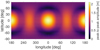 |
Fig. 1 Map of the peak-to-peak amplitude of radial displacement ur of Mercury’ssurface due to tides, assuming h2 = 0.85. |
2 Simulation of measurements
For our simulated laser range measurements, we attempt to account for the most relevant sources of random or systematic errors in a realistic way. We use a topography model for Mercury that is expanded in spherical harmonics up to a degree of 7999, corresponding to a resolution of 958 m. Due to computational limitations, surface roughness at a smaller scale is treated as a random contribution for each individual range measurement. The spacecraft ephemeris and the associated errors in the radial and horizontal components have been obtained from numerical simulations of the Mercury Orbiter Radio science Experiment (MORE). For the instrument range error, we assume a random noise which is independent from shot to shot. The location of the laser footprints is affected by a random pointing jitter, a systematic pointing error, and an error in the assumed libration.
In our simulated measurement campaign, the nominal operation of the MPO begins on March 15, 2026, 4:00 a.m. UTC. Our simulation of the orbit commences with an initial state provided by ESA mission analysis at that epoch. We base the propagation of the orbit on the Hgm005 model of Mercury’s gravity field (Mazarico et al. 2014b), including perturbations by the Sun, tides, and solar radiation pressure. The MPO will have an elliptic orbit with 400 km altitutde at pericenter and 1500 km at apocenter at the start of the science phase.
We simulate nadir-pointing measurements of BELA at a 2 Hz shot frequency. Instrument performance, surface albedo, slope, and roughness, as well as solar noise all influence the signal-to-noise ratio (S/N) of the measurement (Gunderson et al. 2006; Gunderson & Thomas 2010). The S/N affects whether BELA can successfully detect the laser return from ground. Performance modeling has shown that for moderate slopes up to 20° and an albedo of0.19, the probability of false detection is close to zero when the spacecraft altitude is below 1050 km (Steinbrügge et al. 2018b). This is also considered as the nominal maximum operation altitude for BELA. We adapt this threshold for our simulation as a pessimistic scenario, leaving us with 30 282 149 measurements in the one-year nominal mission. The range error is similarly determined by the S/N and is almost never larger than 2 m (Steinbrügge et al. 2018b). We simulatethe range error by adding Gaussian noise with a conservative standard deviation of 2 m to each measurement.
For known spacecraft altitude, the dominant signal contained in the measured altimetric range is the static surface topography. We generate a synthetic topography of Mercury in three steps. First, we use a global DEM derived from stereophotogrammetric data acquired by the Mercury Dual Imaging System (MDIS, Hawkins et al. 2007; Becker et al. 2016) aboard MESSENGER to generate a spherical harmonic model up to degree L. Second, we extrapolate the spherical harmonic model following a power law alb up to degree 7999, where l is the spherical harmonic degree, and a and b are parameters (see Table 1). The spherical harmonic coefficients are randomly distributed around zero with variance  . The spherical harmonic model is transformed into a regular equispaced grid using Féjer quadrature (Schaeffer 2013) and sampled at each measurement location using Lagrange interpolation. Third, Gaussian noise is used to model the topographic power contained in degrees 8000 and higher. The amplitude of this contribution has been determined under the assumption that the spectral power distribution from l = 8000 to infinity is the same as for L < l < 8000.
It is well known that planetary topography at large scales can be described using power laws, reflecting the fractal nature of topography (Turcotte 1987). Previous studies often found that a power law with an exponent − 2.5 < b < −2 approximates the variance spectrum of topography well (Bills & Kobrick 1985; Balmino 1993; Ermakov et al. 2018). At smaller scales, however, it is uncertain if a single power law can be an appropriate representation of topography (Landais et al. 2015). Global data sets have limited resolution and the distribution of morphologies over the surface is inhomogeneous. Therefore, we consider three power laws which are extrapolations of the real topography of Mercury at different scales for our simulations (see Fig. 2 and Table 1). Figure 3 shows large-scale topography and random noise for case 1 (b = −3.3) over the time frame of one orbit of the MPO. The MDIS topography defines most of the large-scale topography. The exponent b = −3.3 is in agreement with the spectral slope of the MDIS topography in the spectral range of 800 < l < 1000, where the results can be considered reliable. We use this as our baseline case. However, to account for a possibly rougher topography at small scale, we also consider the less optimistic cases 2 and 3 which feature spectral slopes that are less steep.
The Mercury Orbiter Radio science Experiment (MORE) determines the orbit of the MPO (Milani et al. 2001; Iess et al. 2009; Imperi et al. 2018). Ground antennas track the MPO with a multifrequency radio link providing range and range rate measurements accurate to 20 cm and 0.04 mm s−1, respectively,at 10 s integration time. The set of synthetic observables used in this simulation comprehends only range-rate measurements (every 10 s) and the Italian Spring Accelerometer (ISA, Iafolla et al. 2010) readings, to cope with mismodeling of all non-gravitational accelerations (Lucchesi & Iafolla 2006). The MPO’s trajectory is retrieved as a solution of the orbit determination process (Tapley et al. 2004, Chap. 4). We used a weighted least-squares filter with a constrained multi-arc approach, consisting of a partitioning of the orbit in consecutive one-day arcs (Imperi et al. 2018). The estimated parameters include the spacecraft state vectors (position and velocity) at the center of the arc, gravity spherical harmonic coefficients up to degree and order 50, the k2 tidal Love number, coefficients describing Mercury’s obliquity and libration, reaction wheels desaturation maneuvers, and calibration parameters for the ISA. The ISA error, driven by thermal variations of the sensing elements, consists of alow frequency (Mercury orbital period, 88 d) and a high frequency (BepiColombo orbital period, 2.3 h) contribution. The first component is modeled by a bias and a bias rate. A new set of these parameters is estimated for every arc. The second component is modeled as a sinusoid at the BepiColombo orbital period. The amplitude of this sinusoid is estimated as a global parameter for the full one-year data set (Iafolla et al. 2007). This approach, followed in Imperi et al. (2018), shall suppress the residual systematic accelerations to a level below 2 × 10⁻⁸ m s−2, which corresponds to a range rate signal well below the expected accuracy (Iess et al. 2009). Residual non-gravitational accelerations at these levels would not introduce any statistically significant bias in the estimated parameters. The numerical simulations of Mariani (2017, Sect. 5.2) also support this assertion. Because ISA readings will not be available during the desaturation maneuvers, additional coefficients describing these maneuvers are estimated.
Unlike range, the range rate (or Doppler) measurements are differential, thus largely immune from systematic errors. In order to account for the uncertainties in the MPO’s trajectory and to provide an ensemble of trajectories to be used in the generation of BELA synthetic observables, we perturb the six components of the spacecraft state vectors of each arc with 100 error realizations. The errors δl in the state vectors are samples of random variables following a multivariate Gaussian distribution,
where Pi is the covariance submatrix of the spacecraft state vector of the ith arc. The standard deviation of the spacecraft position at the center of each arc is shown in Fig. 4. The perturbed initial condition vectors are then propagated up until the beginning of the next arc, thus providing a member of the ensemble of possible MPO trajectories. The difference between these perturbed trajectories and the reference trajectory represents the orbit determination error. It is on the order of a few centimeters in radial direction and meters in transverse and normal directions (Fig. 5), and it is degraded substantially when maneuvers occur during periods without tracking. In fact, after orbit insertion, the MPO will perform daily maneuvers for reaction wheel desaturation and attitude control, but no more orbit maneuvers (Benkhoff et al. 2010). In Fig. 5, the first desaturation maneuver occurring during the navigation passage is estimated well, while the second one is outside the tracking pass and its estimation is limited by the level of the inter-arc constraints (1 m in position). The lateral components of the orbit determination error affect the laser range because the altimeter samples the topography at a different location than the assumed one. Hence, this effect depends on the local topographic slope. The range signal caused by the lateral orbit determination error is typically significantly larger than the radial orbit determination error, which directly affects the range (Fig. 3).
The BELA requirement for the attitude knowledge of the instrument is 20 arcsec. We simulate a 20 arcsec systematic error representinga thermal effect and a 2 arcsec jitter. This is a worst-case assumption because a constant pointing offset, which is less critical for the h2 estimation, is likely to dominate the total attitude knowledge uncertainty. The systematic pointing error is simulated as 20 arcsec × cosM, where M is the mean anomaly of Mercury. It mimics a thermal effect as it is correlated with the Sun-Mercury distance. The direction of the systematic pointing error is randomly chosen but kept constant over the whole mission. The direction of the pointing jitter is randomly chosen for each measurement and its amplitude has a standard deviation of 2 arcsec. The pointing affects the range measurements because the altimeter samples the topography at a different location resulting in a range error on a sloped surface. Theadditional increase in range due to a longer laser path when pointing slightly off-nadir is negligible at an off-nadir angle of 20 arcsec. With increasing spacecraft altitude, the pointing error causes a larger effect. In Fig. 3, the altitude ranges from 1050 km over 400 km back to 1050 km. In our model, for topography case 1, the standard deviation of the range signal caused by pointing misalignment is 3.2 m at perihelion and aphelion.
The second-degree tidal potential is given by (Murray & Dermott 1999),
 (3)
(3)
where μ⊙ = 132712440041.9394 km3 s−2 (Folkner et al. 2014) is the standard gravitational parameter of the Sun, r is the distance between the center of mass of Mercury and the Sun, and ψ is the Mercury-centric angle between the location of the footprint (θ, λ) and the Sun. We access the DE430 ephemerides (Folkner et al. 2014) which allow for the computation of r and ψ with high accuracy using Spacecraft, Planet, Instrument, Camera-matrix, Events (SPICE) kernels (Acton et al. 2018). Higher degrees of the tidal potential are negligibly small. Mercury’s 3:2 spin-orbit resonance causes a permanent tidal bulge which peaks at 35 cm at (0° N, 0° E). We remove the static potential responsible for this tidal bulge using Mercury’s averaged orbital elements a = 57.90909 × 10⁶ km and e = 0.2056317 (Kaula 1964; Stark et al. 2015b). Finally, we use the remaining dynamic potential V2 to compute ur (t) at each measurement location using Eq. (1) and an a priori h2 = 0.8. The tidal displacement measured by the altimeter within one orbit of the spacecraft (Fig. 3) can reach a range of up to 1.4 m when the spacecraft orbits along zero longitude close to perihelion.
We simulate the 88-day libration of Mercury using the des- cription of Mercury’s resonant rotation by Stark et al. (2015b). The amplitude error of the libration is randomly generated and represents the current uncertainty level of 1.3 arcsec. This is a conservative value because the BepiColombo mission is likely to provide an updated estimate with lower uncertainty. A 1.3 arcsec libration translates into a lateral signal of 15 m at the equator, which has a radial effect of up to a few meters. At the poles, the libration has no effect. The correlation between libration and systematic pointing signal in Fig. 3 is due to the similar lateral shift. The right ascension and declination of Mercury will be determined by MORE with uncertainties < 0.2 arcsec, corresponding to an error of <3 m on the surface (Imperi et al. 2018), assuming that the core and solid shell have the same pole. Therefore, the error caused by the uncertainty of the pole orientation is negligible and not considered in this study.
Three power laws used for the simulation of small-scale topography in this study, characterized by the parameters a and b.
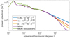 |
Fig. 2 Power spectrum of Mercury’s topography by MDIS (Becker et al. 2016), three simulated spectra based on power laws that extrapolate the MDIS spectrum from different degrees L (see Table 1), and the power spectrum from MLA data and radio science occultations (Neumann et al. 2016). |
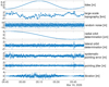 |
Fig. 3 Contributions of each of the simulated signals to range measurements of the altimeter for the time span of one orbit of the MPO, using topography case 1. Libration, pointing, and orbit determination errors contribute to the depicted range measurements mainly through their lateral effect, sampling the topography at a slightly different location. Only measurements with a range < 1050 km are shown. During the depicted time frame, the spacecraft altitude ranges from 1050 km down to 400 km and back to 1050 km. Random noise contains the range error and the Gaussian noise representing small-scale topography. Signals vary for each orbit and each random realization. |
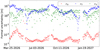 |
Fig. 4 The radial variance component σR, the variance component σN normal to the spacecraft orbital plane, and the transversal variance component σT of the initialpositions for each one-day arc. The figure agrees with Fig. 4 of Imperi et al. (2018). |
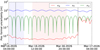 |
Fig. 5 Propagated formal standard deviations of position as a function of time for a typical one-day arc. Quantities σR, σN, and σT indicate theradial component, the component normal to the spacecraft orbital plane, and the transversal component, respectively.The light blue and light red zones depict the X-band (navigation) and Ka-band (scientific) tracking periods, respectively.The black dashed lines indicate the two reaction wheels desaturation maneuvers present on each arc. |
3 Solution strategy
For the simultaneous retrieval of h2 and global topography from the simulated data, we follow the strategy of Koch et al. (2010). A single observation

at co-latitude θk, longitude λk, and time tk is modeled to contain the static topography Tstat at that location, the surface displacement ur, and measurement and model errors ek. Here, (θk, λk) is the simulated spacecraft position, which, in the presence of orbit and pointing errors and an uncertainty in the libration, is slightly offset from the actually sampled position on the ground. The static topography is parametrized as an expansion in local basis functions,
 (6)
(6)
where fi(θk) and fj (λk) are the basis functions and I and J are their number in latitude and longitude direction, respectively, and cij are the basis function coefficients. Koch et al. (2010) used step functions for the basis functions in latitudinal direction fi and compared the use of step functions, piecewise linear functions, and cubic B-splines for the basis functions in longitudinal direction fj. They achieved the best results when applying cubic B-splines and recommended for them to be applied in both directions for further studies. Here we apply cubic B-splines, given by Koch et al. (2010), Eqs. (11) and (14)–(17), as basis functions in both directions. The splines are defined on an equirectangular grid, onto which the topography is projected. The grid cell size is 360°∕J. Since the cells are square, J = 2I. Because the 2D cubic splines are only non-zero within the 16 surrounding grid cells, each spline coefficient cij is only influenced by measurements Tk from 16 gridcells. Compared to spherical harmonics, cubic splines are advantageous because of their locality, which allows for a much highertopography resolution (Steinbrügge et al. 2019). At the same time, splines are smooth enough to model planetary topography well, thus providing a good compromise between global spherical harmonic basis functions on the one hand, and step functions as entirely local basis functions on the other hand.
We solve the observation equation (Eq. (4)) simultaneously for the coefficients cij describing the static topography and for h2 with a regularized least-squares inversion, minimizing

where x is the parameter vector containing the coefficients cij and h2, T is a vector containing the K observations Tk, A is the design matrix resulting from Eq. (4), R is a regularization matrix, and α is the regularization parameter. The regularization serves to stabilize the solution in areas that suffer from limited observations and minimizes the second derivative of the topography at the grid points (θi, λj),
 (7)
(7)
where Sij(θ, λ) = fi(θ)fj(λ) are the 2D cubic B-spline basis functions. We set the regularization parameter α = 10−6K∕(IJ), which allows for a stable solution of the linear equation system, while keeping the inevitable bias on the h2 result small.
4 Results
We generated 100 independent random realizations of measurements as described in Sect. 2. They differ in the topographic model at degrees l > L, direction of the systematic attitude error, synthetic determined orbit, and all other randomly generated error sources. From each of these, we solved for h2 (Sect. 3) using topographic grids of different resolutions. From the resulting 100 h2 values, we computed standard deviation, bias, and root-mean-square error (RMSE; Fig. 6). We first focused on the results achieved using the topography model of case 1. At resolutions lower than 16 grid points per degree, there is a noticeable bias in the results that can be explained by our usage of the MDIS topography model up to degree L = 900. Since there is only a singlerealization of MDIS topography model, the results of 100 random realizations are not distributed evenly around the a priori value of h2 but around a value which is specific to this single random realization. When the topography is modeled by a sufficiently fine grid (≳ 15 grid points per degree) during the solution, the true topography can be almost entirely captured, causing the bias to vanish. Which resolution is sufficiently fine, depends on the degree L up to whichonly a single topography realization is used. The RMSE provides a measure of the 1σ uncertainty at which h2 can be retrieved from the data. It continually decreases with increasing resolution and reaches its minimum at the highest investigated resolution of 28 grid points per degree at a value of ± 0.012.
Next we investigate the influence of different error sources on the uncertainty of h2 in the topography case 1 (Fig. 7). To make the assessment, we generate synthetic data sets where only a single error source is simulated and all other error sources vanish. These simulations include a single realization of topography up to L = 7999 because the lateral components of orbit and pointing errors and the uncertainty in Mercury’s libration only cause a range error when combined with topographic variation. The bias caused by this specific topography realization is subtracted before computing the RMSE presented in Fig. 7. The uncertainty induced by the simulated large-scale topography decreases strongly with increasing resolution as more of it is modeled by the topographic grid. Still, the main source of uncertainty at all resolutions up to 24 grid points per degree is the incomplete representation of the large-scale topography by the splines. This shows the importance of choosing a realistic model for the large-scale topography. The uncertainty induced by systematic misalignment of the instrument becomes the main contributor for resolutions from 24 grid points per degree. At such high resolutions, the cross-track distance will often be larger than the grid resolution. The solution is overparametrized and can therefore fit the perturbed measurements very well instead of smoothing out the perturbations. This is a likely cause for the increase in uncertainty with a denser topographic grid. This trade-off between large-scale topography error and systematic pointing error will eventually lead to an optimal topographic grid resolution. We note that this optimal resolution depends strongly on some of the assumptionstaken, such as the power law used for representing topography at intermediate and small scales, the magnitude of the pointing error, and the specific measurement geometry. For example, we found that an increase of the amplitude of the systematic pointing error by a factor of five will cause an increase in pointing-related h2 uncertainty by a factor of five, resulting in an optimal resolution at about 14 grid cells per degree. If future real data indicates that the pointing error may be large, one should consider adjusting the grid resolution accordingly. Since usually the pointing error is unknown, a weighted average of solutions for different resolutions provides a good estimate of h2.
All other error sources are small in comparison to the large-scale topography and systematic pointing errors. The largest of them is the uncertainty in Mercury’s libration amplitude, followed by the random noise representingrange error and small-scale topography, orbit determination, and finally, pointing jitter. Even though the magnitude of the random noise is much larger than the magnitude of the systematic pointing error and the libration (Fig. 3), the resulting uncertainty is smaller. This shows that the retrieval is only weakly influenced by strong normally distributed noise, but strongly affected by small systematic effects. Similarly, the h2 uncertainty resulting from radial errors in the orbit determination on the order of centimeters is larger than the uncertainty resulting from the lateral component of the orbit determination, which has a magnitude on the order of meters, by a factor of about 3.
Fortunately, we find that none of the modeled error sources cause a systematic bias in the h2 results. However, we note that a much larger than expected systematic pointing error would have the potential to cause such a bias. The longer measured range caused by misalignment by an angle p with respect to the nadir case leads to an error of (1∕ cosp − 1)h on a surface with zero slope, where h is the spacecraft altitude. This error becomes large at perihelion and aphelion, when extreme temperatures cause maximum misalignment. Similarly, the measured tidal displacement reaches maxima at perihelion and aphelion. The maximum tidal displacement is measured over the equator when h ≈ 400 km. For the case of p = 20 arcsec, this corresponds to a radial error of only 1.9 mm, but for p = 100 arcsec, the radial error is 4.7 cm. These radial errors cause a systematic bias of h2 of 0.0012 and 0.027 for p = 20 arcsec and p = 100 arcsec, respectively. While the bias in the former case, representing the maximum expected error, is negligibly small, the latter case illustrates the necessity of high pointing stability. We note that this systematic bias is independent of the grid resolution.
All results discussed so far were obtained using topography case 1 (Table 1). The h2 uncertainties retrieved from case 2 and case 3 at a resolution of 24 grid points per degree are ± 0.017 and ± 0.041, respectively. These values are significantly larger because the topography is less smooth. These cases would benefit from using a topographic grid with higher resolution, because the imperfect modeling of the topography dominates the h2 uncertainty.
 |
Fig. 6 Standard deviation, bias and RMSE of h2 from 100 random realizations as a function of grid resolution for topography case 1 (see Table 1). |
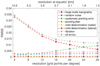 |
Fig. 7 Uncertainty of h2 from simulations as a function of resolution of the topographic grid and its decomposition into the components caused by each of the error sources. The uncertainty is given by the RMSE from 100 random realizations of model and measurement errors. The RMSE induced by pointing jitter and the lateral component of the orbit determination error are both < 0.0004 at all resolutions. |
5 Discussion and conclusions
The results show that the small-scale topography of Mercury is the primary obstacle in accurately measuring its solid body tides. This does not come as a surprise because our initial aim was to detect dm-range radial displacements in measurements taken at different, not perfectly known locations on the surface. While splines model the topography at large scales well, their resolution is not sufficient to model topography at small scales below 1.5 km, which therefore contributes to the measurement uncertainty. This is a fundamental limitation of the measurement method. For simulations, a suitable description of topography at these scales is essential. From Preusker et al. (2017, Fig. 10) we estimate that the MDIS DEM has an effective resolution of at least 15 km, equivalent to L = 511. This justifies using the MDIS topography spectrum to degree L = 450 in topography case 2 and to degree L = 250 in topography case 3. The effective resolution of the MDIS DEM is not globally uniform and may be lower in the southern hemisphere, where images were taken from higher altitudes than in the northern hemisphere. Figure 10 of Preusker et al. (2017) represents a location close to the equator that might represent an average. To our knowledge, no mechanism could cause a flattening of the slope of the spectrum at higher degrees. On the contrary, it seems likely that the spectrum becomes even steeper at higher degrees, as the spectrum derived from the MDIS DEM suggests (Fig. 2). Planetary topography spectra have been found to follow regionally different power laws at scales > 10 km, but power laws with an exponentb ≈−3.4 at scales < 10 km (Aharonson et al. 2001). The power law exponent b = −3.3 used in topography case 1 represents this most likely behavior at small scales.
Nevertheless, even for the two topography cases with flatter slopes, the uncertainty is < 0.05, which is the necessary condition to further constrain interior models. An h2 determination with an accuracy of 0.05 would permit a distinction between a small and a large inner core, whereas an accuracy of 0.01 would allow for a determination of the size of the inner core to about ± 150 km (Steinbrügge et al. 2018a). This value is close to the accuracy limit imposed by other uncertainties in the model of Steinbrügge et al. (2018a). Ultimately, only the global laser altimetric data set acquired by BELA will reveal the spectral slope of Mercury’s topography, which is one of the factors in the obtainable accuracy of h2 determination.
So far, we have used a conservative estimate of instrument performance when assuming that the altimeter only takes measurements at a spacecraft altitude of 1050 km or less. We also carried out a test considering all measurements up to a spacecraft altitude of 1500 km. This modified experiment uses N = 51 800 617 measurements and yields a minimum uncertainty of ± 0.012, which is reached at a resolution of 24 grid points per degree. This shows that an improved instrument performance does not produce significantly better results in terms of h2. A reason for this behavior may be that the pointing error, one of the two dominant error sources, increases with spacecraft altitude. However, in terms of global topography coverage a better performance of BELA is highly desirable.
The MORE radio science investigation will provide a highly accurate estimate of the combined pole orientation of solid inner core and outer shell. If there is evidence for a significant deviation between the orientations of the two poles, future research should investigate the impact of the pole position knowledge on the h2 determination.
An extension of the nominal one-year orbital phase of the MPO by another year might be possible. We also simulate a two-year mission, during which a total of N = 59 630 203 measurements would be taken. The resulting uncertainty is ± 0.010, marking a noticeable improvement over the one-year case. Further extensions of the mission may improve the determination of h2 even more.
Apart from constraining Mercury’s inner core size by measuring its Love number h2, BELA data will also enable a more accurate determination of Mercury’s 88-day libration amplitude ϕ0 and obliquity, which provide additional insights into the interior structure. While the estimation of the retrieval accuracy of ϕ0 from BELA is out of the scope of this study, improved determination from either BELA data alone or a combination of BELA data and imagery can be expected. Stark et al. (2015c,a) derived the current best estimate of the 88-day libration amplitude by co-registering MLA tracks and a terrain model derived from MDIS stereo images. Imperi et al. (2018) also found that the 88-day libration amplitude can be determined with an uncertainty of 0.13 arcsec by BepiColombo’s gravity experiment. The global altimetric coverage achieved with BELA measurements and the reliable orbit determination by MORE will allow for a more accurate determination of geodetic parameters of Mercuryand, therefore, improve the results of Peale’s experiment (Peale 1976). Both a measurement of h2 and improved results from Peale’s experiment would deepen our understanding of Mercury’s interior structure and evolution.
Acknowledgements
R.N.T is supported by grant 50 QW 1401 on behalf of the DLR Space Administration while preparing his PhD thesis in the framework of the International Max Planck Research School on Solar System Science at the University of Göttingen. A.S. was supported by a research grant from Helmholtz Association and German Aerospace Center (DLR) (PD-308). The work of A.D.R., P.C., and L.I. was supported in part by the Italian Space Agency under contract 2017-40-H.0. We thank an anonymous reviewer for their helpful comments.
References
- Acton, C., Bachman, N., Semenov, B., & Wright, E. 2018, Planet. Space Sci., 150, 9 [NASA ADS] [CrossRef] [Google Scholar]
- Aharonson, O., Zuber, M. T., & Rothman, D. H. 2001, J. Geophys. Res. Planets, 106, 23723 [NASA ADS] [CrossRef] [Google Scholar]
- Archinal, B. A., A’Hearn, M. F., Bowell, E., et al. 2011, Celest. Mech. Dyn. Astron., 109, 101 [Google Scholar]
- Balmino, G. 1993, Geophys. Res. Lett., 20, 1063 [NASA ADS] [CrossRef] [Google Scholar]
- Becker, K. J., Robinson, M. S., Becker, T. L., et al. 2016, Lunar Planet. Sci. Conf., 47, 2959 [NASA ADS] [Google Scholar]
- Benkhoff, J., van Casteren, J., Hayakawa, H., et al. 2010, Planet. Space Sci., 58, 2 [NASA ADS] [CrossRef] [Google Scholar]
- Bills, B. G., & Kobrick, M. 1985, J. Geophys. Res. Solid Earth, 90, 827 [CrossRef] [Google Scholar]
- Byrne, P. K., Klimczak, C., Şengör, A. C., et al. 2014, Nat. Geosci., 7, 301 [NASA ADS] [CrossRef] [Google Scholar]
- Cavanaugh, J. F., Smith, J. C., Sun, X., et al. 2007, Space Sci. Rev., 131, 451 [NASA ADS] [CrossRef] [Google Scholar]
- Christensen, U. R. 2006, Nature, 444, 1056 [NASA ADS] [CrossRef] [Google Scholar]
- Dumberry, M., Rivoldini, A., van Hoolst, T., & Yseboodt, M. 2013, Icarus, 225, 62 [NASA ADS] [CrossRef] [Google Scholar]
- Ermakov, A. I., Park, R. S., & Bills, B. G. 2018, J. Geophys. Res. Planets, 123, 2038 [Google Scholar]
- Folkner, W. M., Williams, J. G., Boggs, D. H., Park, R. S., & Kuchynka, P. 2014, The planetary and lunar ephemerides DE430 and DE431, Interplanetary Network Progress Report 42–196, Jet Propulsion Laboratory, Pasadena, CA [Google Scholar]
- Genova, A., Goossens, S., Mazarico, E., et al. 2019, Geophys. Res. Lett., 46, 3625 [NASA ADS] [CrossRef] [Google Scholar]
- Gunderson, K., & Thomas, N. 2010, Planet. Space Sci., 58, 309 [NASA ADS] [CrossRef] [Google Scholar]
- Gunderson, K., Thomas, N., & Rohner, M. 2006, IEEE Trans. Geosci. Remote Sens., 44, 3308 [NASA ADS] [CrossRef] [Google Scholar]
- Hauck, II, S. A., Margot, J.-L., Solomon, S. C., et al. 2013, J. Geophys. Res. Planets, 118, 1204 [NASA ADS] [CrossRef] [Google Scholar]
- Hauck, II, S. A., Grott, M., Byrne, P. K., et al. 2018, in Mercury: the View After Messenger, eds. S. C. Solomon, L. R. Nittler, & B. J. Anderson (Cambridge: Cambridge University Press), 516 [Google Scholar]
- Hawkins, S. E., Boldt, J. D., Darlington, E. H., et al. 2007, Space Sci. Rev., 131, 247 [NASA ADS] [CrossRef] [Google Scholar]
- Hussmann, H., Oberst, J., Stark, A., & Steinbrügge, G. 2018, in Planetary Remote Sensing and Mapping, eds. B. Wu, K. Di, J. Oberst, & I. Karachevtseva (Boca Raton, Florida: CRC Press), 49 [CrossRef] [Google Scholar]
- Iafolla, V., Lucchesi, D. M., Nozzoli, S., & Santoli, F. 2007, Celest. Mech. Dyn. Astron., 97, 165 [NASA ADS] [CrossRef] [MathSciNet] [Google Scholar]
- Iafolla, V., Fiorenza, E., Lefevre, C., et al. 2010, Planet. Space Sci., 58, 300 [NASA ADS] [CrossRef] [Google Scholar]
- Iess, L., Asmar, S., & Tortora, P. 2009, Acta Astronaut., 65, 666 [NASA ADS] [CrossRef] [Google Scholar]
- Imperi, L., Iess, L., & Mariani, M. J. 2018, Icarus, 301, 9 [NASA ADS] [CrossRef] [Google Scholar]
- Kaula, W. M. 1964, Rev. Geophys., 2, 661 [Google Scholar]
- Knibbe, J. S., & van Westrenen, W. 2015, J. Geophys. Res. Planets, 120, 1904 [NASA ADS] [CrossRef] [Google Scholar]
- Knibbe, J. S., & van Westrenen, W. 2017, Icarus, 281, 1 [NASA ADS] [CrossRef] [Google Scholar]
- Koch, C., Christensen, U., & Kallenbach, R. 2008, Planet. Space Sci., 56, 1226 [NASA ADS] [CrossRef] [Google Scholar]
- Koch, C., Kallenbach, R., & Christensen, U. 2010, Planet. Space Sci., 58, 2022 [NASA ADS] [CrossRef] [Google Scholar]
- Landais, F., Schmidt, F., & Lovejoy, S. 2015, Nonlinear Process. Geophys., 22, 713 [NASA ADS] [CrossRef] [Google Scholar]
- Lucchesi, D. M., & Iafolla, V. 2006, Celest. Mech. Dyn. Astron., 96, 99 [NASA ADS] [CrossRef] [MathSciNet] [Google Scholar]
- Margot, J.-L., Peale, S. J., Jurgens, R. F., Slade, M. A., & Holin, I. V. 2007, Sci, 316, 710 [Google Scholar]
- Margot, J.-L., Peale, S. J., Solomon, S. C., et al. 2012, J. Geophys. Res. Planets, 117 [Google Scholar]
- Margot, J.-L., Hauck, II, S. A., Mazarico, E., Padovan, S., & Peale, S. J. 2018, in Mercury: the View After MESSENGER, eds. S. C. Solomon, L. R. Nittler, & B. J. Anderson (Cambridge: Cambridge University Press), 85 [Google Scholar]
- Mariani, Jr., M. 2017, PhD Thesis, Sapienza University of Rome, Rome, Italy [Google Scholar]
- Mazarico, E., Barker, M. K., Neumann, G. A., Zuber, M. T., & Smith, D. E. 2014a, Geophys. Res. Lett., 41, 2282 [NASA ADS] [CrossRef] [Google Scholar]
- Mazarico, E., Genova, A., Goossens, S., et al. 2014b, J. Geophys. Res. Planets, 119, 2417 [NASA ADS] [CrossRef] [Google Scholar]
- Milani, A., Rossi, A., Vokrouhlickỳ, D., Villani, D., & Bonanno, C. 2001, Planet. Space Sci., 49, 1579 [NASA ADS] [CrossRef] [Google Scholar]
- Moore, W. B.,& Schubert, G. 2000, Icarus, 147, 317 [NASA ADS] [CrossRef] [Google Scholar]
- Murray, C. D., & Dermott, S. F. 1999, Solar System Dynamics (Cambridge: Cambridge University Press) [Google Scholar]
- Neumann, G. A., Perry, M. E., Mazarico, E., et al. 2016, Lunar Planet Sci Conf, 47, 2087 [NASA ADS] [Google Scholar]
- Noyelles, B., Frouard, J., Makarov, V. V., & Efroimsky, M. 2014, Icarus, 241, 26 [NASA ADS] [CrossRef] [Google Scholar]
- Padovan, S., Margot, J.-L., Hauck, II, S. A., Moore, W. B., & Solomon, S. C. 2014, J. Geophys. Res. Planets, 119, 850 [NASA ADS] [CrossRef] [Google Scholar]
- Peale, S. J. 1972, Icarus, 17, 168 [NASA ADS] [CrossRef] [Google Scholar]
- Peale, S. J. 1976, Nature, 262, 765 [NASA ADS] [CrossRef] [Google Scholar]
- Preusker, F., Stark, A., Oberst, J., et al. 2017, Planet. Space Sci., 142, 26 [NASA ADS] [CrossRef] [Google Scholar]
- Schaeffer, N. 2013, Geochem. Geophys. Geosyst., 14, 751 [NASA ADS] [CrossRef] [Google Scholar]
- Segatz, M., Spohn, T., Ross, M. N., & Schubert, G. 1988, Icarus, 75, 187 [NASA ADS] [CrossRef] [Google Scholar]
- Solomon, S. C., McNutt, R. L., Gold, R. E., & Domingue, D. L. 2007, Space Sci. Rev., 131, 3 [NASA ADS] [CrossRef] [Google Scholar]
- Stark, A., Oberst, J., Preusker, F., et al. 2015a, Geophys. Res. Lett., 42, 7881 [NASA ADS] [CrossRef] [Google Scholar]
- Stark, A., Oberst, J., & Hussmann, H. 2015b, Celest. Mech. Dyn. Astron., 123, 263 [NASA ADS] [CrossRef] [Google Scholar]
- Stark, A., Oberst, J., Preusker, F., et al. 2015c, Planet. Space Sci., 117, 64 [NASA ADS] [CrossRef] [Google Scholar]
- Stark, A., Oberst, J., Preusker, F., et al. 2018, J. Geod., 92, 949 [NASA ADS] [CrossRef] [Google Scholar]
- Steinbrügge, G., Padovan, S., Hussmann, H., et al. 2018a, J. Geophys. Res. Planets, 123, 2760 [NASA ADS] [CrossRef] [Google Scholar]
- Steinbrügge, G., Stark, A., Hussmann, H., Wickhusen, K., & Oberst, J. 2018b, Planet. Space Sci., 159, 84 [NASA ADS] [CrossRef] [Google Scholar]
- Steinbrügge, G., Steinke, T., Thor, R., Stark, A., & Hussmann, H. 2019, Geoscience, 9, 320 [NASA ADS] [CrossRef] [Google Scholar]
- Tapley, B. D., Schutz, B. E., & Born, G. H. 2004, Statistical Orbit Determination [Google Scholar]
- Thomas, N., Spohn, T., Barriot, J.-P., et al. 2007, Planet. Space Sci., 55, 1398 [NASA ADS] [CrossRef] [Google Scholar]
- Thor, R. N., Kallenbach, R., Gläser, P., et al. 2018, Asia Oceania Geosciences Society (AOGS) 15th Annual Meeting [Google Scholar]
- Turcotte, D. L. 1987, J. Geophys. Res. Solid Earth, 92, E597 [NASA ADS] [CrossRef] [Google Scholar]
- van Hoolst, T., Sohl, F., Holin, I., et al. 2007, in Mercury, eds. A. Balogh, L. Ksanfomality, & R. von Steiger (New York: Springer), 21 [Google Scholar]
- van Hoolst, T., Rivoldini, A., Baland, R.-M., & Yseboodt, M. 2012, Earth Planet. Sci. Lett., 333, 83 [NASA ADS] [CrossRef] [Google Scholar]
- Verma, A. K., & Margot, J.-L. 2016, J. Geophys. Res. Planets, 121, 1627 [NASA ADS] [CrossRef] [Google Scholar]
- Wahr, J. M., Zuber, M. T., Smith, D. E., & Lunine, J. I. 2006, J. Geophys. Res. Planets, 111, E12005 [NASA ADS] [CrossRef] [Google Scholar]
- Wu, X., Bar-Sever, Y. E., Folkner, W. M., Williams, J. G., & Zumberge, J. F. 2001, Geophys. Res. Lett., 28, 2245 [NASA ADS] [CrossRef] [Google Scholar]
All Tables
Three power laws used for the simulation of small-scale topography in this study, characterized by the parameters a and b.
All Figures
|
Fig. 1 Map of the peak-to-peak amplitude of radial displacement ur of Mercury’ssurface due to tides, assuming h2 = 0.85. |
| In the text | |
|
Fig. 2 Power spectrum of Mercury’s topography by MDIS (Becker et al. 2016), three simulated spectra based on power laws that extrapolate the MDIS spectrum from different degrees L (see Table 1), and the power spectrum from MLA data and radio science occultations (Neumann et al. 2016). |
| In the text | |
|
Fig. 3 Contributions of each of the simulated signals to range measurements of the altimeter for the time span of one orbit of the MPO, using topography case 1. Libration, pointing, and orbit determination errors contribute to the depicted range measurements mainly through their lateral effect, sampling the topography at a slightly different location. Only measurements with a range < 1050 km are shown. During the depicted time frame, the spacecraft altitude ranges from 1050 km down to 400 km and back to 1050 km. Random noise contains the range error and the Gaussian noise representing small-scale topography. Signals vary for each orbit and each random realization. |
| In the text | |
|
Fig. 4 The radial variance component σR, the variance component σN normal to the spacecraft orbital plane, and the transversal variance component σT of the initialpositions for each one-day arc. The figure agrees with Fig. 4 of Imperi et al. (2018). |
| In the text | |
|
Fig. 5 Propagated formal standard deviations of position as a function of time for a typical one-day arc. Quantities σR, σN, and σT indicate theradial component, the component normal to the spacecraft orbital plane, and the transversal component, respectively.The light blue and light red zones depict the X-band (navigation) and Ka-band (scientific) tracking periods, respectively.The black dashed lines indicate the two reaction wheels desaturation maneuvers present on each arc. |
| In the text | |
|
Fig. 6 Standard deviation, bias and RMSE of h2 from 100 random realizations as a function of grid resolution for topography case 1 (see Table 1). |
| In the text | |
|
Fig. 7 Uncertainty of h2 from simulations as a function of resolution of the topographic grid and its decomposition into the components caused by each of the error sources. The uncertainty is given by the RMSE from 100 random realizations of model and measurement errors. The RMSE induced by pointing jitter and the lateral component of the orbit determination error are both < 0.0004 at all resolutions. |
| In the text | |
Current usage metrics show cumulative count of Article Views (full-text article views including HTML views, PDF and ePub downloads, according to the available data) and Abstracts Views on Vision4Press platform.
Data correspond to usage on the plateform after 2015. The current usage metrics is available 48-96 hours after online publication and is updated daily on week days.
Initial download of the metrics may take a while.