| Issue |
A&A
Volume 633, January 2020
|
|
|---|---|---|
| Article Number | A29 | |
| Number of page(s) | 14 | |
| Section | Planets and planetary systems | |
| DOI | https://doi.org/10.1051/0004-6361/201936495 | |
| Published online | 03 January 2020 | |
The impact of planet wakes on the location and shape of the water ice line in a protoplanetary disk
1
Institut für Astronomie und Astrophysik, Universität Tübingen,
Auf der Morgenstelle 10,
72076 Tübingen, Germany
e-mail: This email address is being protected from spambots. You need JavaScript enabled to view it.
2
Institute for Theoretical Astrophysics, Zentrum für Astronomie, Heidelberg University,
Albert-Ueberle-Str. 2,
69120 Heidelberg, Germany
3
Research Institute in Astrophysics and Planetology, University of Toulouse,
14 Avenue Edouard Belin,
31400
Toulouse,
France
Received:
10
August
2019
Accepted:
17
October
2019
Abstract
Context. Planets in accretion disks can excite spiral shocks and if these planets are massive enough, they can even open gaps in their vicinity. Both of these effects can influence the overall thermal structure of the disk.
Aims. We model planets of different masses and semimajor axes in disks of various viscosities and accretion rates to examine their impact on disk thermodynamics and to highlight the mutable, non-axisymmetric nature of ice lines in systems with massive planets.
Methods. We conducted a parameter study using numerical hydrodynamics simulations where we treated viscous heating, thermal cooling, and stellar irradiation as additional source terms in the energy equation, with some runs including radiative diffusion. Our parameter space consists of a grid containing different combinations of planet and disk parameters.
Results. Both gap opening and shock heating can displace the ice line, with the effects amplified for massive planets in optically thick disks. The gap region can split an initially hot (T > 170 K) disk into a hot inner disk and a hot ring just outside of the planet’s location, while shock heating can reshape the originally axisymmetric ice line into water-poor islands along spirals. We also find that radiative diffusion does not alter the picture significantly in this context.
Conclusions. Shock heating and gap opening by a planet can effectively heat up optically thick disks and, in general, they can move or reshape the water ice line. This can affect the gap structure and migration torques. It can also produce azimuthal features that follow the trajectory of spiral arms, creating hot zones which lead to “islands” of vapor and ice around spirals that could affect the accretion or growth of icy aggregates.
Key words: protoplanetary disks / planet-disk interactions / planets and satellites: formation / hydrodynamics
© ESO 2019
1 Introduction
Protostellar disks are the birth sites of all sorts of planets. Several observations, such as the discovery of PDS 70b (Keppler et al. 2018) and the recent DSHARP survey (Andrews et al. 2018) have spatially resolved such disks, providing valuable constraints on their composition, structure, and the possible planets they might harbor. Dust continuum observations reveal annular structures and non-axisymmetric features, such as spirals, crescents, or blobs, all of which are consistent with the planet formation scenario (Zhang et al. 2018). According to this scenario, a sufficiently massive planet can trap dust particles by forming pressure maxima (e.g., Ataiee et al. 2018) at radii close to its semimajor axis as it launches density waves in the form of spiral arms that permeate the disk (Ogilvie & Lubow 2002). These pressure traps can allow dust particles to become concentrated enough for their emission to be observable, and also provide an environment for them to collide and grow.
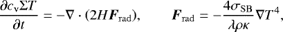
Dust growth is expected to be further facilitated around opacity transition regions (Drążkowska & Alibert 2017; Zhang et al. 2015). Common dust opacity models are, in principle, density-, and temperature-dependent, with boundaries defined at conditions where aggregates of certain composition change phase to the extent that crossing between two opacity regimes can change the absorption and emission properties of the disk. For example, the water content of ice-coated particles sublimates at the so-called water ice line around Tice ≈ 170 K (Lin & Papaloizou 1985), with small variations depending on model assumptions. This temperature marks the first opacity transition threshold that particles will cross as they drift inwards according to several opacity models (e.g., Bell & Lin 1994; Semenov et al. 2003). Since water can only be found on particles outside of this ice line, its location can provide insight and constraints on the origin of water content for planetesimals and young planets in an evolving protostellar disk, depending on the disk’s temperature profile (Bitsch et al. 2019).
The disk’s thermal structure depends on the balance between heating and cooling terms. Kley & Crida (2008) show that accounting for radiation transport, instead of treating the disk as locally isothermal, can have significant effects on the migration of super-Earths by slowing down or even reversing the migration rate. Additionally, Rafikov (2016) shows that shock heating due to planet-induced spirals can be a significant heat source in the inner few au of the disk. Evidently, the optically thick region near the star can reach high densities and temperatures, which could lead to an important contribution by shock heating to the energy content of the disk.
In this study, we investigate the conditions under which planet shock heating can significantly raise temperatures and the degree to which spirals can affect the location and shape of the water ice line. Based on our findings, we speculate about the possible implications for dust and planetesimal growth around the ice line.
In Sect. 2, we calculate an estimate for the amount of heat a planet can pump into the disk through shock heating. Our physical framework, as well as the numerical setup, is described in Sect. 3. In Sects. 4 and 5, we present our results regarding the disk structure and ice line shape, respectively. In Sect. 6, we comment on our findings and discuss their potential implications, while Sect. 7 contains a summary of our work, along with our conclusions.
2 Shock heating
Planet-induced spiral arms form as a result of density waves shearing in the Keplerian disk flow as they propagate away from the planet (Kley & Nelson 2012). They are overdensities with respect to the disk “background” (azimuthally-averaged) profile that can steepen into shocks as they travel through the disk (Goodman & Rafikov 2001). In an adiabatic framework, we can expect a pressure jump at the location of the shock, which can lie close to the planet (Zhu et al. 2015). This pressure jump can generate heat near the planet, potentially affecting the temperature profile near the corotating region. Thus, the question is how important this shock heating can be when compared to other heat sources in the disk (e.g., viscosity and stellar irradiation).
In order to get an idea of the prominence of spiral shocks as a heat-generating mechanism, it is worthwhile to first estimate their contribution theoretically and compare it to other sources of heat in the disk. We follow a line of thought similar to that of Rafikov (2016) and calculate the heating by an adiabatic spiral shock for an assumed density jump at the shock.
Heating by a spiral shock can be considered as a three-phase process: (1) heating by the shocks; (2) decompression; and (3) settling to the pre-shock density. In this subsection, we refer to the pre-shock quantities (before phase 1) by the subscript 1, to the decompression phase by subscript 2, and to the post-shock state by subscript 3. The following calculation is performed in the shock’s comoving frame. The shock heating rate can be estimated by calculating the specific internal energy difference between phase 1 and phase 3 for each passage of the shock and then dividing it by the time between two passages. Knowing the pressure p and surface density Σ in each of the three phases, we can calculate the specific internal energy via e = p∕(Σ(γ − 1)). The classical jump condition and equation of state can give us the values for all necessary quantities. In our calculations, we use the surface density  instead of the density ρ. Note that the jump conditions are also valid if ρ is replaced by Σ because during the shock, the disk does not have enough time to expand vertically and change the local density. This allows us to use two-dimensional (2D) hydrodynamic simulations to test the predictions of this analytical model.
When the shock hits the pre-shock gas between phase 1 and phase 2, the density and pressure at the second phase can be given by the Rankine–Hugoniot jump condition that reads
![Mathematical equation: \begin{eqnarray} \frac{\Sigma_2}{\Sigma_1} &=& \frac{(\gamma+1) \mathcal{M}_{1}^2}{(\gamma-1)\mathcal{M}_{1}^2+2},\\[4pt] \frac{p_2}{p_1} &=& \frac{2 \gamma \mathcal{M}_{1}^2-(\gamma-1)}{\gamma+1}\end{eqnarray}](/articles/aa/full_html/2020/01/aa36495-19/aa36495-19-eq2.png)
where γ is the adiabatic index and  denotes the Mach number.
The decompression between phase 2 and phase 3 can be either adiabatic or isothermal depending on disk cooling. If the shocks are in the optically thin part of the disk, the inserted energy can be easily radiated away, the post-shock temperature returns to its pre-shock value rapidly (except in a very narrow region of the shock itself), and the decompression would be isothermal. Conversely, in the optically thick part of the disk where the energy cannot quickly escape, the decompression is adiabatic. Because we are interested in the cases where shocks heat the disk up and change its temperature structure, we choose the adiabatic decompression. Therefore, the pressure and density before and after decompression can be given by an adiabatic equation of state as
 (3)
(3)
Because the gas density will return to its pre-shock value, we can replace Σ3 with Σ1 so that:
 (4)
(4)
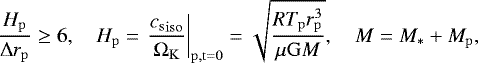
Let us assume that the time between two passages of a shock through a specific location of radius r in the disk is tpass = 2π∕|ΩK(r) − ΩK(rp)|, where  is the Keplerian frequency, G the gravitational constant, M* and Mp the masses of the star and planet respectively, and rp the planet’s semimajor axis. The amount of heat per unit time (averaged over many passages) is then:
![Mathematical equation: \begin{eqnarray*} \begin{split} \hspace*{-2pt}Q_{\textrm{sh}} &=\frac{\Delta (\Sigma e)}{\Delta t}=\frac{e_3-e_1}{t_{\textrm{pass}}} \Sigma_{1} = \frac{1}{t_{\textrm{pass}}(\gamma-1)}\left[p_2 \left(\frac{\Sigma_1}{\Sigma_2}\right)^{\gamma} - p_1 \right]. \end{split} \end{eqnarray*}](/articles/aa/full_html/2020/01/aa36495-19/aa36495-19-eq7.png) (5)
(5)
Expressing  from Eq. (1) we obtain:
 (6)
(6)
Inserting this into Eq. (2), we can remove p2 from the above equation and obtain:
![Mathematical equation: \begin{equation*}Q_{\textrm{sh}}= \frac{p_1}{t_{\mathrm{pass}}(\gamma-1)} \times \left[\left(\frac{1}{\sigma}\right)^{\gamma} \frac{(\gamma+1)\sigma- (\gamma-1)}{(\gamma+1)-(\gamma-1)\sigma} -1\right], \end{equation*}](/articles/aa/full_html/2020/01/aa36495-19/aa36495-19-eq10.png) (7)
(7)
where σ := Σ2∕Σ1 is the “shock strength”. This equation is identical to Eq. (16) of Rafikov (2016) assuming a one-armed spiral. In the literature, there is no straightforward way to find the strength of planetary spirals. Following Rafikov (2016), we take σ as a free parameter and compare the shock heating rate with the viscous and the irradiation heating rates. This comparison is shown in Fig. 1, where we artificially damp σ exponentially with distance from the planet’s gap opening region to avoid overestimating shock heating far from the planet:
![Mathematical equation: \begin{equation*}\sigma(r) = \begin{cases} \sigma, & |r-r_{\mathrm{p}}|\leq 2.5\,{\textrm{R}_{\textrm{Hill}}}, \\[3pt] 1+(\sigma-1)e^{-4(|r-r_{\mathrm{p}}|-2.5\,{\textrm{R}_{\textrm{Hill}}})/r_{\mathrm{p}}}, & \text{otherwise}, \end{cases} \end{equation*}](/articles/aa/full_html/2020/01/aa36495-19/aa36495-19-eq11.png) (8)
(8)
where ![Mathematical equation: ${\textrm{R}_{\textrm{Hill}}}\equiv \sqrt[3]{M_{\mathrm{p}}/3M_{\ast}}\,r_{\mathrm{p}}$](/articles/aa/full_html/2020/01/aa36495-19/aa36495-19-eq12.png) .
.
For  , Eq. (1) gives an upper limit to shock strength for adiabatic shocks as
  for γ =7∕5. We should note that this upper limit is not strict if additional thermal mechanisms (such as cooling) are included in the models.
This estimate shows that shock heating by a planet can overcome the other two heating sources if the planet is massive enough to produce strong shocks, and the disk opacity is large enough to prevent heat from quickly escaping from the midplane. This extra heating raises the temperature in the disk up to the location where the shocks damp greatly. Because the disk opacity also depends on temperature (see Fig. 2), spiral heating by a planet in the vicinity of an ice line (either via migration or in-situ formation) might displace the latter. In the following sections, we study this problem for a more realistic model with shocks that are not necessarily adiabatic and examine how much and under what conditions the location and shape of an ice line can change.
 |
Fig. 1 Shock heating rate by planet’s spirals estimated by method in Sect. 2 and damped using Eq. (8) for different shock strengths (σ = Σ2∕Σ1, γ =7∕5) compared to viscous and irradiative heating rates (dashed and solid black lines; see Sect. 3.1). Lilac band indicates the corotating region, in which the estimates are not valid due to potential gap opening. The model used for this plot assumes Mp = 100 M⊕, Ṁ = 10−8 M⊙ yr−1, α = 10−3, rp = 4 au (see Sects. 3.1 and 3.2). |
 |
Fig. 2 First four opacity regimes according to Lin & Papaloizou (1985). Dotted teal line marks the water ice line (Tice = 170 K). Different branches are patched together by interpolation. |
3 Model setup
In this section, we present the physical framework that we utilize in our planet–disk modeling. We describe the relevant equations and the assumptions behind them, along with our numerical setup as far as our parameter space, initial and boundary conditions, and grid structures are concerned.
3.1 Physics
We solve the vertically integrated Navier–Stokes equations for a disk with surface density Σ, velocity vector v and vertically integrated specific internal energy e on a polar coordinate system {r, ϕ} centered around the star. For a perfect gas, the equations read
![Mathematical equation: \begin{eqnarray*}&& \hspace*{-6pt} {\frac{\mathrm{d}{\Sigma}}{\mathrm{d}{t}}} =-\Sigma\nabla\cdot\bm{v}, \nonumber\\[4pt] && \hspace*{-6pt} \Sigma {\frac{\mathrm{d}{v}}{\mathrm{d}{t}}} =-\nabla p-\Sigma\nabla\Phi+\nabla\cdot{\overline{\bm{{\Sigma}}}}, \nonumber \\[4pt] && \hspace*{-6pt} {\frac{\mathrm{d}{\Sigma e}}{\mathrm{d}{t}}} =-\gamma\Sigma e\nabla\cdot\bm{v}+Q_{\mathrm{visc}}+Q_{\mathrm{irr}}-Q_{\mathrm{cool}}, \end{eqnarray*}](/articles/aa/full_html/2020/01/aa36495-19/aa36495-19-eq15.png) (9)
(9)
where γ =7∕5 is the adiabatic index, p = (γ − 1)Σe is the vertically integrated pressure and  denotes the viscous stress tensor.
The adiabatic and isothermal sound speeds cs,  are related as:
 (10)
(10)
where H is the pressure scale height, h = H∕r is the aspect ratio and  is the Keplerian azimuthal velocity. The universal gas constant and mean molecular weight are denoted by R and μ = 2.353, respectively.
Source terms Qvisc, Qirr, and Qcool in the energy equation correspond to viscous heating, stellar irradiation, and thermal cooling, respectively:
![Mathematical equation: \begin{eqnarray*}&& \hspace*{-6pt} Q_{\mathrm{visc}}=\frac{1}{2\nu\Sigma}\left(\sigma_{rr}^2+2\sigma_{r\phi}^2+\sigma_{\phi\phi}^2\right)+\frac{2\nu\Sigma}{9}\left(\nabla\cdot\bm{v}\right)^2, \nonumber \\[4pt] && \hspace*{-6pt} Q_{\mathrm{irr}}=2\frac{L_{\ast}}{4{\pi} r^2}(1-\epsilon)\left( {\frac{\mathrm{d}{\log H}}{\mathrm{d}{\log r}}}-1 \right)h\frac{1}{\tau_{\mathrm{eff}}}, \nonumber \\[4pt] && \hspace*{-6pt} Q_{\mathrm{cool}}=2\sigma_{\mathrm{SB}}\frac{T^4}{\tau_{\mathrm{eff}}}, \end{eqnarray*}](/articles/aa/full_html/2020/01/aa36495-19/aa36495-19-eq20.png) (11)
(11)
where ν = αcsH is the kinematic viscosity according to the α-viscosity model of Shakura & Sunyaev (1973), σSB is the Stefan–Boltzmann constant, and τeff is an effective optical depth following Hubeny (1990):
 (12)
(12)
with the Rosseland mean opacity κ(ρ, T) defined according to Lin & Papaloizou (1985), shown in Fig. 2. The correction factor c1 =1∕2 is added following Müller & Kley (2012) to account for the drop in opacity with height. We assume a Gaussian vertical density profile so that  .
.
As far as irradiation is concerned, we assume a star of solar luminosity L* =L⊙ and a disk albedo of ɛ =1∕2. Following Menou & Goodman (2004), the factor  is assumed to be constant and equal to 9∕7 (i.e., disk self-shadowing is not considered).
3.2 Numerics
We utilized the numerical MHD code PLUTO (Mignone et al. 2007) for our simulations, along with the FARGO algorithm described by Masset (2000) and implemented as a library into PLUTO by Mignone et al. (2012). To enable radiative diffusion, we implemented a separate module that is briefly described in Appendix D. Simulations with an embedded planet were run on a polar {r, ϕ} grid, logarithmically spaced in the radial direction.
Our parameter space is shown in Table 1. It contains the planet mass Mp, the planet’s semimajor axis rp (fixed, circular orbits), the viscosity parameter α and the initial disk mass accretion rate Ṁ, which is constant throughout the disk in viscous equilibrium such that Ṁ = 3πνΣ (Lodato 2007). By selecting an α value and a constant accretion rate we can then construct well-defined equilibrium states.
To generate our initial conditions, we prepared 1D models that satisfy viscous and thermal equilibrium conditions:
 (13)
(13)
and ruled out very cold disks or gravitationally unstable ones, for which the Toomre parameter QT (Toomre 1964), defined as:
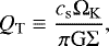 (14)
(14)
is less than unity. The initial profiles we used are plotted in Fig. 3.
We then embedded planets in each configuration and ran each model until the disk reached, roughly, its viscous and thermal equilibrium or a maximum simulated time of tmax = 105 years elapses. To ensure a constant Ṁ through the boundaries, Σ, v were damped to the initial profiles according to de Val-Borro et al. (2006) over a timescale of 0.3 boundary orbital periods.
The gravitational forces read
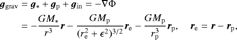 (15)
(15)
where g*, gp, gin refer to the gravitational acceleration by the star, the planet, and the indirect term that arises due to the star–planet system orbiting around their mutual barycenter. The planet is on a fixed orbit and we neglected the backreaction of the disk onto star and planet. For the softening length, we used ɛ = 0.6H to prevent singularities around the planet’s location. The value 0.6 was selected according to Müller et al. (2012) as it provides very similar results to 3D models. We note that ɛ was evaluated using the local H at each cell.
Parameter space: rp is quoted in au and Ṁ in M⊙ yr−1.
 |
Fig. 3 Initial profiles for five disk models with different Ṁ and α used throughout this study. Dotted pink line refers to an inviscid disk where Qcool =Qirr (i.e., the irradiation temperature) and functions as our effective temperature floor. It becomes clear that viscous heating is strongest in the inner disk, while irradiation dominates its outer parts. |
Grid setup.
4 Disk profiles
Having described our physics and numerical methods, we proceeded to execute our simulations. The grid setup for each model is shown in Table 2. A cross-code comparison as well as a resolution test for the verification of our numerical setup is provided in Appendix A. We constructed the numerical grid such that the pressure scale height H is resolved by at least six grid cells at the planet’s location (see Appendix B for more details).
We first investigated the thermal input of a planet onto the disk and the structure of the gap that planet might possibly carve. In order to do so, we first presented some comparisons of the gap width and depth across different models for both surface density and temperature. We then highlighted the influence of disk aspect ratio and viscosity on the planet’s ability to open a gap. We then determined to show temperature profiles for various disks with identical initial temperatures so that the planet’s impact would become more apparent.
Afterwards, we took a closer look at the structure of spiral arms by tracking the same quantities along their crests and compared them against the azimuthally averaged disk profiles. This would give us an estimation for both the temperature contrast between the spirals and the disk, as well as the shock strength along those spirals.
 |
Fig. 4 Azimuthally-averaged profiles of surface density (left) and temperature (right) across planet masses and locations for our models. More massive planets open deeper and wider gaps but the temperature inside the gap region is not necessarily lower in the outer, irradiation-dominated disk due to stellar irradiation. The dotted pink line marks the disk irradiation temperature (Qcool = Qirr). |
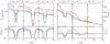 |
Fig. 5 Azimuthally-averaged profiles of surface density (left) and temperature (right) around planet’s location across different disk models for Mp = 100 M⊕. These snapshots are taken once each model has reached a quasi-equilibrium state, meaning that the gap depth is not well-defined for very low viscosities. However, it only takes a few hundred orbits for the overall disk structure to equilibrate. |
4.1 Gap opening capabilities of a planet
In Fig. 4, we compare the gap-opening capabilities of planets of different masses for our fiducial model (Ṁ = 10−8, α =10−3). While the least massive planet in these models (10 M⊕) does not open a gap, the rest are sufficiently massive to show a clear trend between planet mass and gap width, with more massive planets opening deeper and wider gaps.
However, we also find that there is a lower limit to the temperatures inside the gap. This arises due to stellar irradiation, which provides enough heat to form an effective temperature floor where Qirr= Qcool. This term overpowers other heating effects with increasing radii and, as a result, a temperature gap is not visible in the outer disk regardless of planet mass.
Then, for a given planet mass of Mp = 100 M⊕, we carried out the same comparison across models with different disk parameters. The results are shown on Fig. 5, where a similar behavior is visible for temperatures inside the gap.
A key point in these findings is that we observed shallower gaps for higher values of α (for a given Ṁ) or Ṁ (for a given α). This can beunderstood by looking at the two main mechanisms determining the gap edge, as shown by Crida et al. (2006): viscosity and pressure gradients. Before adding a planet to a disk of a given Ṁ and α, one can show that Ṁ ∝ νΣ ∝ αpr3∕2, such that pressure gradients are stronger in disks with a higher Ṁ or lower α. This, combined with the fact that viscous dissipation is scaled with α, allows for easier gap opening in disks witheither a higher Ṁ or lower α. This is nothing new, as it has been pointed out by Crida et al. (2006), Zhang et al. (2018) as well as in previous studies, that disks with a lower viscosity or aspect ratio support the gap opening process.
4.2 Spiral shock heating by a planet
On the right panels of Figs. 4 and 5, apart from the depth (or lack thereof) of a gap, we noted a temperatureincrease on both sides of the planet’s vicinity, sometimes by a factor of 1.5–2 compared to the initial profiles. This heat excess is scaled with planet mass and it can lead to quite high temperatures in the inner disk. This pattern is in agreement with our theoretical estimates, given in Sect. 2, based on which we should expect that the optically thick inner disk is moresusceptible to heating by spiral shocks.
In the attempt to compare the individual effect of each of our four parameters – planet mass, accretion rate, viscosity parameter, and planet radius – we plotted pairs of models where three out of four parameters are the same, allowing us to quantify theinfluence of the fourth. The trends we find with this method are clear enough that a comparison between our fiducial model and four other models suffices to convey the general picture. This comparison is shown in Fig. 6.
The common denominator for these four panels is the cooling timescale of different disks and the regions within them. We can get a rough estimate of this timescale by focusing on the cooling term in Eq. (11) and writing
 (16)
(16)
which further backs the assumption that the deciding factor in determining the contribution of shock heating to the thermal budget of the disk is the optical depth. Finally, we compared two models where {Ṁ = 10−8, α = 10−2} and {Ṁ = 10−9, α = 10−4}, respectively. These two models happen to have identical initial temperature profiles but they show the lowest and highest optical depths in our suite of simulations, respectively. This comparison is plotted in Fig. 7 and clearly shows the effect of optical depth on the contribution of shock heating. It should be noted that even though the optically thinnest model in that figure shows only small traces of excess heat due to shocks, the cooling timescale is still more than 10% of the orbital period at 10 au and, therefore, radiative effects of the disk should still be treated self-consistently to get a correct picture of its evolution.
From our results, we can conclude that shock heating is, in principle, important for all of our models and that it sometimes dominates when the cooling timescale of the disk is sufficiently long. This implies that planets with semimajor axes in the range of 1–10 au can noticeably heat up their environment through spiral shocks and, as a result, an adiabatic equation of state is necessary when modeling planet–disk interaction in this regime.
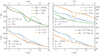 |
Fig. 6 Azimuthally-averaged temperature profiles for four pairs of models, showcasing influence of each of four variables in our parameter space (Mp, Ṁ, α, rp) on spiral shock heating. Our fiducial model (Mp = 100 M⊕, Ṁ = 10−8, α = 10−3, rp = 4) is shown in blue on every panel, while dashed lines depict initial profiles of the model of corresponding color. In all cases, we noted stronger shock heating in optically thicker regions of the disks. This behavior can also be seen in the rest of our suite of models. |
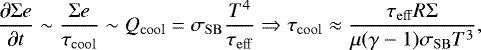
4.3 Spiral arm structure and shock strength
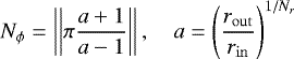
In the previous section, we discuss the effect of shock heating by comparing azimuthally-averaged profiles in simulations with and without planets. While this is a useful approximation to form a general image of planet–disk interaction, it cannot isolate the contributionof individual spirals or their properties. Inspired by the approach of Zhu et al. (2015) we wrote a script that can trace spiral arms as they propagate away from the planet and logged their coordinates, as well as Σarm and Tarm along their crests. We then used this data to estimate a proxy for the shock strength along those spirals as  (shown in Sect. 2), as well as their pitch angles β defined as tanβ = dlograrm∕dϕarm.
As in the previous section, trends among models are clear enough such that we do not need to present results for our entire library of simulations. Instead, we take into account that the contribution of shock heating is scaled with the optical depth and show results for three regimes: the optically thinnest model (Ṁ = 10−8, α = 10−2, rp = 10), the optically thickest one (Ṁ = 10−9, α = 10−4, rp = 1), as well as our fiducial model (Ṁ = 10−8, α = 10−3, rp = 4), which also happens to lie somewhere in the middle. For each model, we calculate the shock strength and pitch anglesof primary spirals (i.e., those that connect to the planet). Since the pitch angle is scaled with h far from thelaunching point according to linear theory, we also plotted the azimuthally-averaged aspect ratio  .
.
In an attempt to filter out unphysical shock strength values inside the low-density ring around the planet, we calculated the half-width of the horseshoe region as shown in Paardekooper et al. (2010):
 (17)
(17)
as well as the shock length following Dong et al. (2011):
 (18)
(18)
where  is the disk thermal mass. If Mp > Mth, then xs = 0 (spirals shock immediately upon launch). For more massive planets, where a gap opens, we set a cut-off where |r − rp|≤ 2.5 RHill. We then excluded data from within any of those three regions.
Our results are summarized in Fig. 8. We see that the shock strength of spirals typically lies between 1.5–3 for massive planets but rarely exceeds 1.5 for 10 M⊕ models. Looking at Fig. 1, we can see that such shocks produce competitive heating when compared to either viscosity or stellar irradiation for rp ≤ 4. In the rp = 10 case (see the left panels of Fig. 8), however, the planet is embedded in an optically thin, irradiation-dominated region and, as a result, shock heating is overcome by stellar irradiation, which eventually sets the overall profile.
As far as pitch angles are concerned, we attempted to fit their curves with analytical formulas that assume an aspect ratio profile. In the inner disk, due to the temperature being defined by different power laws depending on the opacity regime, it is easier to assume that the aspect ratio is roughly constant and use the formula by Ogilvie & Lubow (2002) to calculate the location of spirals
![Mathematical equation: \begin{equation*}\phi_{\mathrm{arm}} = -\mathrm{sgn}(r-r_{\mathrm{p}}) \frac{2}{3h}\left[\left(\frac{r}{r_{\mathrm{p}}}\right)^{3/2}-\frac{3}{2}\ln \left(\frac{r}{r_{\mathrm{p}}}\right)-1\right]. \end{equation*}](/articles/aa/full_html/2020/01/aa36495-19/aa36495-19-eq33.png) (19)
(19)
On the other hand, for the irradiation-dominated outer disk (where Qirr≊ Qcool), we can utilize the formula by Muto et al. (2012):
![Mathematical equation: \begin{eqnarray*}\phi_{\mathrm{arm}} &=& -\frac{\mathrm{sgn}(r-r_{\mathrm{p}})}{h_{\mathrm{p}}} \nonumber \\ && \times \left[ \left(\frac{r}{r_{\mathrm{p}}}\right)^{1+\eta}\left\{\frac{1}{1+\eta}-\frac{1}{1-\zeta+\eta}\left(\frac{r}{r_{\mathrm{p}}}\right)^{-\zeta}\right\}\right. \nonumber \\ && \left.-\left(\frac{1}{1+\eta}-\frac{1}{1-\zeta+\eta}\right)\right], \end{eqnarray*}](/articles/aa/full_html/2020/01/aa36495-19/aa36495-19-eq34.png) (20)
(20)
where ΩK ∝ r−ζ and h ∝ r0.5−η. For h ∝ r2∕7 (see Eq. (11)), we have ζ =3∕2 and η =3∕14.
Even when utilizing both formulas, we find that it is difficult to get a good fit and that we always underestimate the pitch angles. This shows that the heating generated by the planets’ spirals can change the disk aspect ratio such that it cannot be accurately approximated with a power law. The fit completely breaks down for massive planets or optically thick disks, where we find that pitch angles are inflated around the location of planets. This makes sense since shock heating peaks at these locations (e.g., see Figs. 1 and 5).
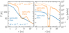 |
Fig. 7 Azimuthally-averaged temperature and cooling timescale for two models that share the same initial temperature profile but have very different optical depth profiles. We see that shock heating is significantly stronger for the optically thicker model, while the optically thinner one looks almost unchanged. |
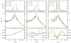 |
Fig. 8 Shock strength, pitch angles, and azimuthally-averaged aspect ratios for three representative models. Optical depth and cooling timescale increase from left to right. Top: shocks are stronger for more massive planets but their dependence on disk parameters is not clear. To filter out unphysical results, we mask points that lie within the gap region (|r − rp |≤ 2.5 RHill) or the corotating region (see Eq. (17)). Middle: pitch angles are roughly the same regardless of planet mass for the optically thin case but deviate with increasing optical depth. Black lines denote the expected values using Eq. (19) for h = hp (dashed) or Eq. (20) for h = hpr2∕7 (dotted). Bottom: a power law fit of aspect ratio is only possible for optically thin case or low mass planets but fidelity for such a fit breaks down even for 10-Earth-mass planets in an optically thick disk. Black dashed lines refer to initial aspect ratio profiles. |
5 Location and shape of the water ice line
Using the analytical estimates in Sect. 2, we show that if a massive planet is located in the optically thick part of the disk, the shocks are adiabatic and spiral heating can increase the temperature of the disk. In Sect. 4, we present our results on the heating potential of these shocks through our numerical simulations, confirming our estimates. In this section, we investigate how much a planet can displace ice lines (e.g., the water ice line) in a disk. Our motivation to do so lies inquantifying the possibility that a planet can starve itself or the inner disk of water as it forms, as well as the possibility that it can impact the environment in which planetesimals could grow (Drążkowska & Alibert 2017).
From Fig. 2 it becomes clear that the Rosseland mean opacity is independent of density up to T ≈103 K such that the water ice line effectively represents the temperature where ice sublimates. This implies that the location of the ice line does not explicitly depend on the density jump across shocks but instead on the temperaturethey can reach. In this study, we follow Lin & Papaloizou (1985) and define the water ice line rice as the point where the temperaturereaches Tice = 170 K (see opacity transition at this point in Fig. 2).
5.1 Location of the azimuthally-averaged water ice line
In the absence of a planet and assuming an axisymmetric disk, the equation r = rice defines a circle with radius rice from the star, within which water can only be found in the form of vapor. For now, let us assume that the presence of the planet does not significantly perturb the ice line in the azimuthal direction but instead moves it uniformly towards or away from the star, such that the new location of the ice line is  once equilibrium is reached.
Depending on its initial location, the ice line is susceptible to two planet-induced phenomena: the closer it lies next to the planet, the more it is exposed to shock heating from the latter, leading to a larger outward displacement as the planet heats up its surroundings. In the extreme case that the ice line initially lies directly next to the planet, it can be pushed away by a factor of 1.5 or even more (see Fig. 9a). The impact on the location of the ice line is scaled with the mass of the planet, with Jupiter-sized planets increasing  by a factor of 2.
However, in the case that the planet is massive enough to open a gap, embedding it too close to the ice line such that the latter overlaps with the optically thin gap region results in a recession of the ice line towards the inner gap edge (see Fig. 9b). In this case, the final location of the ice line depends on the width of the gap, which is also scaled with planet mass.Of course, for planets of sufficiently low mass, a gap will not open and, therefore, the ice line location will essentially remain intact.
Finally, it is possible that gap opening and shock heating can compete for the determination of the location of the ice line. This behavior is shown on Fig. 9c: shock heating initially moves the ice line outwards, “pulling” it closer to the planet. However, the slower gap opening process eventually “catches up” and the steep temperature gradient near the inner gap edge extends the region affected by the gap down to around 2.5 au (0.6rp), returning the ice line to a location similar to its initial one once the gap has fully opened.
5.2 Azimuthal structure of the ice line
In the previous section, we consider the ice line as an axisymmetric line – a circle with radius  around the star – by tracking its location using azimuthally-averaged temperature profiles. However, shock heating is a strongly non-axisymmetric process as it follows the trajectories of spiral arms. Therefore, its influence on the location of the ice line should introduce azimuthal features on the latter. In other words, the full picture is 2D – at least within the scope of this project.
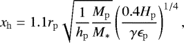
To examine the azimuthal structure of the ice line, we plot temperature maps of our models at equilibrium and draw contours at T(r, ϕ) = Tice. We summarize the results for some of our representative models in Fig. 10.
In general, a few key behaviors can be observed in our simulation results. The ice line tends to move outwards in optically thick disks (as shown above) and deform it in such a way that it follows the trajectories of spirals when strong shocks are present. Therefore, we can distinguish a few distinct “extremes.” For a low-mass planet in an optically thin disk, the location or shape of the ice line do not change. In an optically thick disk, the same planet might slightly move the ice line outwards or perturb it along the azimuthal axis.
In both of these cases, the analysis in Sect. 5.1 still applies with good accuracy. However, a massive planet launches strong shocks and opens a gap which can halt the outward movement of the ice line or even cause it to recede to the inner gap edge. Therefore, for a high-mass planet in an optically thin disk (where typically  ), we see hot spirals form in the inner disk (such that Tarm > Tice) but we see little to no radial displacement of the ice line (see Fig. 10b). If initially
  , the ice line will recede to the inner gap edge, in addition to forming hot spirals in the outer disk (see Fig. 10c).
On the other hand, for a massive planet in an optically thick disk, shock heating is strong enough to displace the ice line to the outer disk to the point where spiral pitch angles are small and the spirals are very tightly wound, heating the disk uniformly in azimuth. In this case, the domain is split into a hot inner disk, a cold gap, and a hot ring in the outer disk (see Fig. 10a). If initially  , the ice line will again recede to the inner gap edge while possibly forming hot spirals or a hot ring in the outer disk, depending on the optical depth.
Of course, if  , far out at the irradiation-dominated outer disk, the ice line will not change in shape or location but a cold ring can still form inside the gap region. However, the optical depth rapidly increases at small distances from the star and, as such, the pile-up of inner spiral arms by a Jupiter-sized planet can still cause substantial heating, moving the ice line outwards even in optically thinner models (as shown in Fig. 9d).
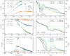 |
Fig. 9 Azimuthally-averaged ice line location for three sample models, showcasing three possible evolution scenarios, panel a: spiral heating pushes ice line outwards; panel b: ice line recedes to the inner gap edge; panel c: shock heating initially pushes ice line outwards but eventually a gap is carved and ice line recedes inwards. These effects are amplified for more massive planets. It should be noted that in the case of a cold gap, ice can recondense within the gap region (panel a). |
6 Discussion
In this section we discuss our findings with respect to their possible impact on the growth and change of orbital elements of the planets, andon the structure of the disk.
6.1 A shift of the ice line
Under certain conditions (low Ṁ, low α), a planet located at 1 au could push the ice line outwards by a few au. This leads to a reduction of icy solid material present in the disk in terms of size and number. This lowers the accretion of solid material onto the planet as more matter is in gaseous form, which has a lower (viscous) drift than embedded particles. On the other hand, when the snow line moves just a little beyond the planet, icy aggregates that may fall apart can release tiny silicate grains (Schoonenberg et al. 2018) and tiny dust may be less well trappedin the outer edge of the planet gap, possibly affecting the accretion of dust onto the planet. The net effect will be an enhancement of dry over wet particle accretion onto the planet and a reduction of the water content in the inner regions of the disk.
6.2 Slush islands
In our simulations, we locate regions where the conditions within the disk are such that the temperature along the spirals is above the ice sublimation threshold and drops below it between spiral crests (see Fig. 10). Ice sublimates around the peak of the shock but condenses again further away from it, such that along the boundary of the spiral (as defined by the ice line) one might find a mixture of ice and water vapor with a “slushy” consistency, hence, we call them “slush islands.” These may occur inside as well as outside of the planet’s location. The repetitive sublimationand condensation will slow down dust growth as growing particles will periodically be reduced in size.
6.3 Migration torques
The disk heating of an embedded planet will change the torques acting on it and, hence, affect its migration rate. As the torques are scaled inversely to the disk’s scale height (Kley & Nelson 2012), it is expected that the planets slow down due to the heating they produce. This possibility has already been explored and discussed by Hallam & Paardekooper (2018), who show that even a simplistic prescription of gap edge illumination can result in the slowing down or even reversing of the migration rate of planets. In light of our results concerning the planets’ ability to heat up their vicinity through spiral shocks, our modeling supports the findings of that study in that regard.
6.4 Temperature within the gap
In our simulations the temperature within the gap is lower that the environment because of the reduced optical depth. For deep gaps, the irradiation temperature was reached. Previous works look at the gas temperature in a planet’s gap (via radiative transfer calculations) while considering the three dimensional vertical extent of the disk (Jang-Condell & Turner 2012). In that particular study, the gap’s temperature is determined by shadowing and illumination effects, which are not included in our 2D treatment of irradiation. It was also found that the outer gap edge, which is directly exposed to starlight, can heat the interior of the gap to the extent that the temperature can rise even higher than the ambient temperature.
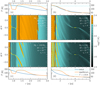 |
Fig. 10 Temperature maps for four models, showcasing azimuthal structure of ice line. Two colormaps denote the blue “cold” (T < Tice) and orange “hot” (T > Tice) disk, respectively, with a yellow line separating the two regions (T = Tice). The initial location of the ice line (before a planet is embedded) is marked with a dotted white line, while its azimuthally-averaged location in equilibrium is shown with a dashed white line. |
6.5 Simplifications and assumptions
Throughout our study, we have made several assumptions about the various physical processes at play. Therefore, we find that it is importantfor us to draw attention to the potential impact they can have on our results.
First and foremost, there is our two-dimensional approximation in simulating global, adiabatic disks. Lyra et al. (2016) point out that theadditional degree of freedom in the vertical expansion of an adiabatic shock results in overall weaker shocks, suggesting that our results overestimate shock heating. This can be amended by “scaling” our results to refer to more massive planets.
Secondly, regarding the smoothing length chosen for the planet’s gravitational potential, we chose to evaluate the scale height locally (H(r, ϕ)) instead of using that at the planet’s location (Hp). The reason behind this choice is that it corrects for the disk’s finite thickness, as shown by Müller et al. (2012). However, this assumption might be problematic in radiative simulations. For example, the planet’s accretion luminosity can result in a “hot bubble” around the planet (Klahr & Kley 2006), where the scale height can increase sharply with respect to its initial value. Nevertheless, this smoothing length becomes important at a scale far smaller than the planet’s Hill radius and, therefore, it should have a minuscule effect on the latter’s gravitational potential.
Additionally, our model of stellar irradiation contains a simplification in that disk self-shadowing is ignored. Specifically, we assume that the star illuminates a disk where the scale height does not significantly change (such that  is constant and refers to a power-law profile for H) but then we point out that shock heating can, in fact, strongly affect said disk property. While this assumption leads to a very straightforward and stable numerical implementation of stellar irradiation, it occasionally results in a disparity between our assumption of 9∕7 for
  and the actual value. This disparity is greater for optically thick disks and diminishes with the increasing distance from the star. We can, therefore, justify our choice by remembering that stellar irradiation is indeed a dominant heat source at large radii, where the approximation holds best, and gives way to viscous and shock heating near the star, rendering it insignificant regardless of how well the approximation holds.
7 Conclusions
In our study, we examined the thermodynamical impact of planets on the ambient protoplanetary disk in which they are embedded. In order to do so, we first calculated an estimate for the amount of heat a planet can deliver into the disk through spiral shocks and we showed that such heating can be significant. We noted that this process is strongest in the immediate vicinity of the planet but it also has the potential to influence a larger area depending on disk optical depth. We then carried out a grid of 2D numerical hydrodynamics simulations with included radiative effects in order to find out if and how much this planet-generated heating can influence the disk and displace or deform the otherwise axisymmetric water ice line, defined as the radius rice, where T(rice) = Tice = 170 K.
We find that spiral shock heating is most important in optically thick, viscosity-dominated disks. Both of these requirements suggest a long cooling timescale, and they are fulfilled in the inner few au of a protoplanetary disk. On the other hand, the irradiation-dominated outer disk suppresses shock heating by raising the aspect ratio. However, even when a planet is embedded in the outer disk, its inner spirals can heat up the disk as they propagate inwards.
We also show that both a high viscosity or aspect ratio inhibit the gap opening process, a result which is consistent with previous studies. On top of that, treating radiative effects allows us to probe the gas temperature inside the gap region. We find that in the inner disk, where viscous heating determines the gas temperature, a cold gap can be seen around massive planets. This is not visible in the outer disk, where the temperature both inside and out of the gap region is determined by the irradiation temperature.
By tracing the planet’s spiral arms we find that planet-induced spiral shocks are scaled in strength with planet mass to the extent that shock heating is strongest for massive planets. This leads to a noticeable difference between spiral and background temperatures, with clear implications on the pitch angles of said spirals. We also show that due to the fact that the aspect ratio can increase dramatically by high-mass planets, fitting pitch angles with a standard flaring-aspect-ratio prescription would not, in principle, yield accurate results when shock heating is important.
Subsequently, we investigated the planet’s ability to displace the water ice line. We found that shock heating by the planet can increase temperatures high enough to push the ice line away from the star. This outward displacement of the ice line can happen to various degrees depending on the optical depth of the disk. Optically thicker disks are unable to efficiently radiate away excess heat and are prone to larger ice line displacements. Shock heating can then lead to either a uniform outward movement or a non-axisymmetric deformation of the ice line.
In the inner few au of our disks, planets that are massive enough to carve a gap can create a cold ring around their semimajor axis. This gap cooling effect can easily overpower shock heating in the immediate vicinity of the planet, pulling the ice line inwardsto the inner gap edge if it was initially near the soon-to-be-opened gap region or creating a “hot ring” outside of the planet’s location if the ice line maintains a radius greater than that of the planet’s semimajor axis.
However, it is also possible that the ice line becomes deformed due to the temperature contrast between spirals and the disk background to the extent that it bends to follow spiral trajectories. This deformation is clearest for strong shocks in optically thin disks, wherethe ice line can trace the inner or outer spirals depending on the initial disk temperature profile. Such spirals will then be water-poor, with possible implications on dust growth in their vicinity. These effects can impact the accretion rate and composition of accreted particles on a planet.
As far as the scale of this displacement and deformation is concerned, we find that planet mass plays a leading role in determining both shock strength as well as gap width to the extent that any effect related to the location or shape of the ice line is amplified for higher planet masses.
Finally, we report that accounting for radiative diffusion in the disk midplane leads to no significant differences in temperatureprofiles or ice line deformation. In addition, it leads to barely any observable differences in azimuthally-averaged ice line locations and spiral arm opening angles. As a result, radiative diffusion can be safely ignored in the context of this study.
Acknowledgements
The authors thank the referee for the constructive comments and suggestions for improving the quality of the manuscript. S.A. acknowledges support from the Swiss NCCR PlanetS. C.P.D. and W.K. acknowledge funding from the DFG research group FOR 2634 “Planet Formation Witnesses and Probes: Transition Disks” under grant DU 414/22-1 and KL 650/30-1. We acknowledge the support of the DFG priority program SPP 1992 “Exploring the Diversity of Extrasolar Planets” under grant KL 650/27-1. The authors acknowledge support by the High Performance and Cloud Computing Group at the Zentrum für Datenverarbeitung of the University of Tübingen, the state of Baden–Württemberg through bwHPC and the GermanResearch Foundation (DFG) through grant no INST 37/935-1 FUGG. This research was supported by the Munich Institute for Astro- and Particle Physics (MIAPP) of the DFG cluster of excellence “Origin and Structure of the Universe”. All plots in this paper were made with the Python library matplotlib (Hunter 2007).
Appendix A Grid and code validation and physics justification
In order to verify our setup, we ran a comparison test against the numerical hydrodynamics code FARGO (Masset 2000). For this test, we simulated the first 6250 orbits (50 kyr) for a fiducial model (Mp = 100 M⊕, rp = 4au, Ṁ = 10−8 M⊙ yr−1, α =10−3) using PLUTO, then transferred the current, quasi-equilibrium disk state to FARGO and ran it for an additional 650 orbits using both codes and using exactly the same physics. The final disk state for surface density and temperature is plotted in Fig. A.1. We find that the two codes produce similar results in the inner and outer disk, differing only around the planet. We rationalize this by pointing out the fundamentally different treatment of shocks between the two codes: PLUTO utilizes a Godunov-type scheme (a conservative, finite-volume approximation combined with a Riemann solver) that captures and resolves shocks with very good accuracy, in contrast to FARGO’s treatment of shocks.
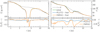 |
Fig. A.1 Comparison between PLUTO and FARGO, after restarting from identical disk state in quasi-equilibrium (ti = 6250 orbits) and running independently until tf = ti + 650 orbits. Both surface density and temperature profiles are in good agreement across codes in the outer disk, while the different treatment of shock heating between the codes becomes evident only near to the planet. |
Overall, the level of agreement between the two codes provides good grounds to assume that our setup is working as intended and that we can proceed with simulating our suite of models using PLUTO.
Next, we verified our grid size. We used enough cells in the radial direction such that the pressure scale height H is resolved by six or more cells at the planet’s location. We used an appropriate grid size in the azimuthal direction to maintain square cells (roughly twice the number of radial cells). To check whether this grid size was large enough, we reran our fiducial model with double the resolution on both the r and ϕ axes (using PLUTO) and compared the azimuthally-averaged surface density and temperature profiles (see Fig. A.2). The results turned out to be quite similar (to roughly 90%) so for our qualitative study this resolution of six cells per scale height is justified. The grid size used for our simulations is shown in Table 2.
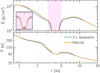 |
Fig. A.2 Two runs for our fiducial model, one of which (blue curves) has double resolution on both r and ϕ axes (for total of four times as many cells). The snapshots are taken at t = 100 kyr (12 500 orbits) where equilibrium has more or less been reached. The inset zooms in on the pink-tinted region, showcasing the match between the two gap profiles. |
Finally, we investigated the influence of radiative diffusion on the phenomena we intended to study, namely the shock strength of planetary spirals and the influence of the planet’s shock heating on the water ice line. We find that accounting for radiative diffusion within the disk midplane barely affected the outcome of the two simulations. It was enabled in the fiducial model for Mp = 10 and 100 M⊕ so that a case where no gap opens can also be studied. We report on the effect of radiative diffusion for these two models in more detail in Appendix C.
Appendix B Grid structure
As described in Sect. 3.2, our first step was to generate 1D models for various combinations of Ṁ and α. These models were calculated for r ∈ [0.2, 100] au and then an appropriate region was selected depending on planet semimajor axis rp by constructing a grid that mimics the PLUTO grid structure and fitting our initial profiles onto it through linear interpolation. That grid typically extends from rp ∕5–5rp except for simulations with 10 M⊕ planets, which were carried out earlier with a domain always between 0.5–20 au regardless of planet location. A verification test was carried out to make sure that that setup did not affect the quality of the simulations and produced results identical to those using the former setup, therefore these simulations did not need to be rerun.
As far as grid size is concerned, we measured the pressure scale height Hp at the planet’s location and constructed a logarithmically-spaced array of Nr cells in the r-direction that satisfies:
 (B.1)
(B.1)
while the number of cells in the azimuthal direction was chosen so that cells are square, or:
 (B.2)
(B.2)
This typically results in grids of around 600 × 1200 cells (e.g., our fiducial model with Mp = 100 M⊕, Ṁ = 10−8 M⊙ yr−1, α =10−3, rp = 4 au contains 531 × 1037 cells).
Appendix C Effect of radiative diffusion
We repeated two simulations for our fiducial model (rp = 4au, Ṁ = 10−8 M⊙ yr−1, α =10−3) with flux-limited diffusion (FLD) enabled in the disk midplane. This additional term should smear out peaks in the temperature structure of the disk and could become important along the trajectories of spirals. We choose Mp ∈{10, 100} M⊕ to examine its overall impact on the disk whether a gap is carved or not. However, we do not see a significant difference in the low- nor in the high-mass simulations except for the lower peak temperature of spirals in the FLD models and a slight inward movement of the ice line. This implies that vertical cooling happens at a much faster rate than the planar diffusion timescale. By comparing their timescales, we indeed find that thermal cooling readjusts disk temperatures roughly 100 times faster than radiative diffusion does (except for inside the gap region) to the extent that its effect on temperature profiles and the ice line is negligible.
Disk profiles and spiral arms
A comparison is plotted in Fig. C.1 for the high-mass case. Spiral arms show slightly lower temperature maxima and the azimuthally-averaged temperature profile is smoother overall, with lower highs and higher lows. This effect is strongest around parts of the disk that might contain steep temperature gradients, such as the region between 2.5–3.5 au for these models, but it still barely makes a difference of more than 3% with respect to the model where we did not account for radiative diffusion, leading to identical aspect ratios in the two models and, therefore, practically indistinguishable pitch angles along spirals. We note that for the 10-Earth-mass case, differences between the two models are much smaller.
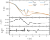 |
Fig. C.1 Comparison between two variants of our fiducial model (Mp = 100 M⊕), with and without radiative diffusion enabled. The effect of diffusion is visible near steep gradients along spiral crests or the gap edges but negligible in general. Spiral arms in both models overlap exactly, as shown in the bottom panel. |
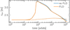 |
Fig. C.2 Evolution of ice line location for two pairs of simulations with and without treatment of radiative diffusion. Solid and dashed lines refer to models where Mp = 10 and 100 M⊕, respectively. |
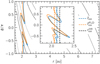 |
Fig. C.3 Shape of water ice line at equilibrium for two models with and without radiative diffusion (Mp = 100 M⊕). Aside from the slight inward shift of the ice line, its shape is generally unaffected. Here we plot an extended range of our simulation for context. Solid, dashed, and dotted black curves mark the location of primary, secondary, and tertiary spirals, respectively. |
Locationand shape of the ice line
Temperature gradients are slightly different when accounting for radiative diffusion, and especially so around the gap edge. Since the ice line is relatively close to said gap edge in the two models where the module is enabled, we are more or less looking at the effects of radiative diffusion at its maximum potential. However, in the previous paragraph, we report that its effect barely changes the picture with regard to shock strength, gap width, or spiral location. Because of these three points, the ice line’s location over time is expected to be slightly, but not significantly, different when compared to that found in our standard simulations.
In Fig. C.2, we compare the location of  over time between our standard models and their respective FLD-enabled models. Indeed, the softer temperature profile in the inner disk allows the ice line to recede slightly more inwards when radiative diffusion is enabled. Nevertheless, the effect is still minuscule for the high-mass case and negligible for the low-mass case.
A 2D analysis of the ice line’s shape offers similar results. As shown in Fig. C.3, accounting for radiative diffusion does not change the shape of the ice line with respect to the standard model, but, instead, it shifts it slightly inwards, as shown in Fig. C.2. As with the 1D analysis, this difference is practically nonexistent for the low-mass case as the temperatureprofile is softer overall: shocks by the 10-Earth-mass planet are significantly weaker and a gap does not open.
Appendix D Implementation of radiative diffusion
To examine the effect of radiative diffusion along the disk midplane, we implemented an external module that is coupled with PLUTO and solves the following equation after every timestep:
 (D.1)
(D.1)
where F denotes the radiation flux across the disk midplane and is defined as:
 (D.2)
(D.2)
where λ is a flux limiter, following Kley (1989).
By defining a diffusion coefficient K as
 (D.3)
(D.3)
we discretize Eq. (D.1) following Appendix A.1 in Müller (2014)
 (D.4)
(D.4)
on a grid where i and j denote cell indices along the r- and ϕ-direction respectively, and obtain:
 (D.5)
(D.5)
where n and n + 1 denote the states at time t and t + Δt, respectively.
We now have to solve for Tn+1. We can group up the right hand side to form a linear system:
 (D.6)
(D.6)
where
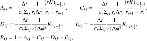 (D.7)
(D.7)
are elements of the matrix  . We solve this system using successive overrelaxation (SOR). Therefore, we calculate and fix
  before iterating over:
![Mathematical equation: \begin{equation*} \begin{split} \hspace*{-2pt}\tilde{T}_{i,j}^{k+1}=&\,(1-\omega)\tilde{T}_{i,j}^{k}\\ &-\,\frac{\omega}{B_{ij}}\left[A_{ij}\tilde{T}_{i-1,j}^{k}+C_{ij}\tilde{T}_{i+1,j}^{k}+D_{ij}\tilde{T}_{i,j-1}^{k}+E_{ij}\tilde{T}_{i,j+1}^{k}-T_{i,j}^{k=0}\right], \end{split} \end{equation*}](/articles/aa/full_html/2020/01/aa36495-19/aa36495-19-eq56.png) (D.8)
(D.8)
with ω = 1.5 until  converges. Boundary conditions during this iterative process are closed in order to conserve total thermal energy through the radiative diffusion substep.
References
- Andrews, S. M., Huang, J., Pérez, L. M., et al. 2018, ApJ, 869, L41 [NASA ADS] [CrossRef] [Google Scholar]
- Ataiee, S., Baruteau, C., Alibert, Y., & Benz, W. 2018, A&A, 615, A110 [NASA ADS] [CrossRef] [EDP Sciences] [Google Scholar]
- Bell, K. R., & Lin, D. N. C. 1994, ApJ, 427, 987 [NASA ADS] [CrossRef] [Google Scholar]
- Bitsch, B., Raymond, S. N., & Izidoro, A. 2019, A&A, 624, A109 [NASA ADS] [CrossRef] [EDP Sciences] [Google Scholar]
- Crida, A., Morbidelli, A., & Masset, F. 2006, Icarus, 181, 587 [Google Scholar]
- de Val-Borro, M., Edgar, R. G., Artymowicz, P., et al. 2006, MNRAS, 370, 529 [NASA ADS] [CrossRef] [Google Scholar]
- Dong, R., Rafikov, R. R., & Stone, J. M. 2011, ApJ, 741, 57 [NASA ADS] [CrossRef] [Google Scholar]
- Drążkowska, J., & Alibert, Y. 2017, A&A, 608, A92 [NASA ADS] [CrossRef] [EDP Sciences] [Google Scholar]
- Goodman, J., & Rafikov, R. R. 2001, ApJ, 552, 793 [NASA ADS] [CrossRef] [Google Scholar]
- Hallam, P. D., & Paardekooper, S. J. 2018, MNRAS, 481, 1667 [NASA ADS] [CrossRef] [Google Scholar]
- Hubeny, I. 1990, ApJ, 351, 632 [NASA ADS] [CrossRef] [Google Scholar]
- Hunter, J. D. 2007, Comput. Sci. Eng., 9, 90 [NASA ADS] [CrossRef] [Google Scholar]
- Jang-Condell, H., & Turner, N. J. 2012, ApJ, 749, 153 [NASA ADS] [CrossRef] [Google Scholar]
- Keppler, M., Benisty, M., Müller, A., et al. 2018, A&A, 617, A44 [NASA ADS] [CrossRef] [EDP Sciences] [Google Scholar]
- Klahr, H., & Kley, W. 2006, A&A, 445, 747 [NASA ADS] [CrossRef] [EDP Sciences] [Google Scholar]
- Kley, W. 1989, A&A, 208, 98 [NASA ADS] [Google Scholar]
- Kley, W., & Crida, A. 2008, A&A, 487, L9 [NASA ADS] [CrossRef] [EDP Sciences] [Google Scholar]
- Kley, W., & Nelson, R. P. 2012, ARA&A, 50, 211 [NASA ADS] [CrossRef] [Google Scholar]
- Lin, D. N. C., & Papaloizou, J. 1985, in Protostars and Planets II, eds. D. C. Black, & M. S. Matthews (Tucson: University of Arizona Press), 981 [Google Scholar]
- Lodato, G. 2007, Rivista del Nuovo Cimento, 30, 293 [NASA ADS] [Google Scholar]
- Lyra, W., Richert, A. J. W., Boley, A., et al. 2016, ApJ, 817, 102 [NASA ADS] [CrossRef] [Google Scholar]
- Masset, F. 2000, A&AS, 141, 165 [NASA ADS] [CrossRef] [EDP Sciences] [Google Scholar]
- Menou, K., & Goodman, J. 2004, ApJ, 606, 520 [NASA ADS] [CrossRef] [Google Scholar]
- Mignone, A., Bodo, G., Massaglia, S., et al. 2007, ApJS, 170, 228 [Google Scholar]
- Mignone, A., Flock, M., Stute, M., Kolb, S. M., & Muscianisi, G. 2012, A&A, 545, A152 [NASA ADS] [CrossRef] [EDP Sciences] [Google Scholar]
- Müller, T. W. A. 2014, PhD Thesis, University of Tuebingen, Tuebingen, Germany [Google Scholar]
- Müller, T. W. A., & Kley, W. 2012, A&A, 539, A18 [NASA ADS] [CrossRef] [EDP Sciences] [Google Scholar]
- Müller, T. W. A., Kley, W., & Meru, F. 2012, A&A, 541, A123 [NASA ADS] [CrossRef] [EDP Sciences] [Google Scholar]
- Muto, T., Grady, C. A., Hashimoto, J., et al. 2012, ApJ, 748, L22 [NASA ADS] [CrossRef] [Google Scholar]
- Ogilvie, G. I., & Lubow, S. H. 2002, MNRAS, 330, 950 [NASA ADS] [CrossRef] [Google Scholar]
- Paardekooper,S. J., Baruteau, C., Crida, A., & Kley, W. 2010, MNRAS, 401, 1950 [NASA ADS] [CrossRef] [Google Scholar]
- Rafikov, R. R. 2016, ApJ, 831, 122 [NASA ADS] [CrossRef] [Google Scholar]
- Schoonenberg,D., Ormel, C. W., & Krijt, S. 2018, A&A, 620, A134 [NASA ADS] [CrossRef] [EDP Sciences] [Google Scholar]
- Semenov, D., Henning, T., Helling, C., Ilgner, M., & Sedlmayr, E. 2003, A&A, 410, 611 [NASA ADS] [CrossRef] [EDP Sciences] [Google Scholar]
- Shakura, N. I., & Sunyaev, R. A. 1973, A&A, 500, 33 [Google Scholar]
- Toomre, A. 1964, ApJ, 139, 1217 [Google Scholar]
- Zhang, K., Blake, G. A., & Bergin, E. A. 2015, ApJ, 806, L7 [NASA ADS] [CrossRef] [Google Scholar]
- Zhang, S., Zhu, Z., Huang, J., et al. 2018, ApJ, 869, L47 [NASA ADS] [CrossRef] [Google Scholar]
- Zhu, Z., Dong,R., Stone, J. M., & Rafikov, R. R. 2015, ApJ, 813, 88 [NASA ADS] [CrossRef] [Google Scholar]
All Tables
All Figures
|
Fig. 1 Shock heating rate by planet’s spirals estimated by method in Sect. 2 and damped using Eq. (8) for different shock strengths (σ = Σ2∕Σ1, γ =7∕5) compared to viscous and irradiative heating rates (dashed and solid black lines; see Sect. 3.1). Lilac band indicates the corotating region, in which the estimates are not valid due to potential gap opening. The model used for this plot assumes Mp = 100 M⊕, Ṁ = 10−8 M⊙ yr−1, α = 10−3, rp = 4 au (see Sects. 3.1 and 3.2). |
| In the text | |
|
Fig. 2 First four opacity regimes according to Lin & Papaloizou (1985). Dotted teal line marks the water ice line (Tice = 170 K). Different branches are patched together by interpolation. |
| In the text | |
|
Fig. 3 Initial profiles for five disk models with different Ṁ and α used throughout this study. Dotted pink line refers to an inviscid disk where Qcool =Qirr (i.e., the irradiation temperature) and functions as our effective temperature floor. It becomes clear that viscous heating is strongest in the inner disk, while irradiation dominates its outer parts. |
| In the text | |
|
Fig. 4 Azimuthally-averaged profiles of surface density (left) and temperature (right) across planet masses and locations for our models. More massive planets open deeper and wider gaps but the temperature inside the gap region is not necessarily lower in the outer, irradiation-dominated disk due to stellar irradiation. The dotted pink line marks the disk irradiation temperature (Qcool = Qirr). |
| In the text | |
|
Fig. 5 Azimuthally-averaged profiles of surface density (left) and temperature (right) around planet’s location across different disk models for Mp = 100 M⊕. These snapshots are taken once each model has reached a quasi-equilibrium state, meaning that the gap depth is not well-defined for very low viscosities. However, it only takes a few hundred orbits for the overall disk structure to equilibrate. |
| In the text | |
|
Fig. 6 Azimuthally-averaged temperature profiles for four pairs of models, showcasing influence of each of four variables in our parameter space (Mp, Ṁ, α, rp) on spiral shock heating. Our fiducial model (Mp = 100 M⊕, Ṁ = 10−8, α = 10−3, rp = 4) is shown in blue on every panel, while dashed lines depict initial profiles of the model of corresponding color. In all cases, we noted stronger shock heating in optically thicker regions of the disks. This behavior can also be seen in the rest of our suite of models. |
| In the text | |
|
Fig. 7 Azimuthally-averaged temperature and cooling timescale for two models that share the same initial temperature profile but have very different optical depth profiles. We see that shock heating is significantly stronger for the optically thicker model, while the optically thinner one looks almost unchanged. |
| In the text | |
|
Fig. 8 Shock strength, pitch angles, and azimuthally-averaged aspect ratios for three representative models. Optical depth and cooling timescale increase from left to right. Top: shocks are stronger for more massive planets but their dependence on disk parameters is not clear. To filter out unphysical results, we mask points that lie within the gap region (|r − rp |≤ 2.5 RHill) or the corotating region (see Eq. (17)). Middle: pitch angles are roughly the same regardless of planet mass for the optically thin case but deviate with increasing optical depth. Black lines denote the expected values using Eq. (19) for h = hp (dashed) or Eq. (20) for h = hpr2∕7 (dotted). Bottom: a power law fit of aspect ratio is only possible for optically thin case or low mass planets but fidelity for such a fit breaks down even for 10-Earth-mass planets in an optically thick disk. Black dashed lines refer to initial aspect ratio profiles. |
| In the text | |
|
Fig. 9 Azimuthally-averaged ice line location for three sample models, showcasing three possible evolution scenarios, panel a: spiral heating pushes ice line outwards; panel b: ice line recedes to the inner gap edge; panel c: shock heating initially pushes ice line outwards but eventually a gap is carved and ice line recedes inwards. These effects are amplified for more massive planets. It should be noted that in the case of a cold gap, ice can recondense within the gap region (panel a). |
| In the text | |
|
Fig. 10 Temperature maps for four models, showcasing azimuthal structure of ice line. Two colormaps denote the blue “cold” (T < Tice) and orange “hot” (T > Tice) disk, respectively, with a yellow line separating the two regions (T = Tice). The initial location of the ice line (before a planet is embedded) is marked with a dotted white line, while its azimuthally-averaged location in equilibrium is shown with a dashed white line. |
| In the text | |
|
Fig. A.1 Comparison between PLUTO and FARGO, after restarting from identical disk state in quasi-equilibrium (ti = 6250 orbits) and running independently until tf = ti + 650 orbits. Both surface density and temperature profiles are in good agreement across codes in the outer disk, while the different treatment of shock heating between the codes becomes evident only near to the planet. |
| In the text | |
|
Fig. A.2 Two runs for our fiducial model, one of which (blue curves) has double resolution on both r and ϕ axes (for total of four times as many cells). The snapshots are taken at t = 100 kyr (12 500 orbits) where equilibrium has more or less been reached. The inset zooms in on the pink-tinted region, showcasing the match between the two gap profiles. |
| In the text | |
|
Fig. C.1 Comparison between two variants of our fiducial model (Mp = 100 M⊕), with and without radiative diffusion enabled. The effect of diffusion is visible near steep gradients along spiral crests or the gap edges but negligible in general. Spiral arms in both models overlap exactly, as shown in the bottom panel. |
| In the text | |
|
Fig. C.2 Evolution of ice line location for two pairs of simulations with and without treatment of radiative diffusion. Solid and dashed lines refer to models where Mp = 10 and 100 M⊕, respectively. |
| In the text | |
|
Fig. C.3 Shape of water ice line at equilibrium for two models with and without radiative diffusion (Mp = 100 M⊕). Aside from the slight inward shift of the ice line, its shape is generally unaffected. Here we plot an extended range of our simulation for context. Solid, dashed, and dotted black curves mark the location of primary, secondary, and tertiary spirals, respectively. |
| In the text | |
Current usage metrics show cumulative count of Article Views (full-text article views including HTML views, PDF and ePub downloads, according to the available data) and Abstracts Views on Vision4Press platform.
Data correspond to usage on the plateform after 2015. The current usage metrics is available 48-96 hours after online publication and is updated daily on week days.
Initial download of the metrics may take a while.