| Issue |
A&A
Volume 633, January 2020
|
|
|---|---|---|
| Article Number | A5 | |
| Number of page(s) | 17 | |
| Section | Extragalactic astronomy | |
| DOI | https://doi.org/10.1051/0004-6361/201936481 | |
| Published online | 19 December 2019 | |
Magnetic fields and cosmic rays in M 31
I. Spectral indices, scale lengths, Faraday rotation, and magnetic field pattern⋆⋆⋆
Max-Planck-Institut für Radioastronomie, Auf dem Hügel 69, 53121 Bonn, Germany
e-mail: This email address is being protected from spambots. You need JavaScript enabled to view it.
, This email address is being protected from spambots. You need JavaScript enabled to view it.
, This email address is being protected from spambots. You need JavaScript enabled to view it.
Received:
8
August
2019
Accepted:
16
October
2019
Abstract
Context. Magnetic fields play an important role in the dynamics and evolution of galaxies; however, the amplification and ordering of the initial seed fields are not fully understood. The nearby spiral galaxy M 31 is an ideal laboratory for extensive studies of magnetic fields.
Aims. Our aim was to measure the intrinsic structure of the magnetic fields in M 31 and compare them with dynamo models of field amplification.
Methods. The intensity of polarized synchrotron emission and its orientation are used to measure the orientations of the magnetic field components in the plane of the sky. The Faraday rotation measure gives information about the field components along the line of sight. With the Effelsberg 100-m telescope three deep radio continuum surveys of the Andromeda galaxy, M 31, were performed at 2.645, 4.85, and 8.35 GHz (wavelengths of 11.3, 6.2, and 3.6 cm). The λ3.6 cm survey is the first radio survey of M 31 at such small wavelengths. Maps of the Faraday rotation measures (RMs) are calculated from the distributions of the polarization angle.
Results. At all wavelengths the total and polarized emission is concentrated in a ring-like structure of about 7–13 kpc in radius from the centre. Propagation of cosmic rays away from the star-forming regions is evident. The ring of synchrotron emission is wider than the ring of the thermal radio emission, and the radial scale length of synchrotron emission is larger than that of thermal emission. The polarized intensity from the ring in the plane of the sky varies double-periodically with azimuthal angle, indicating that the ordered magnetic field is oriented almost along the ring, with a pitch angle of −14 ° ±2° at λ6.2 cm. The RM varies systematically along the ring. The analysis shows a large-scale sinusoidal variation with azimuthal angle, signature of an axisymmetric spiral (ASS) regular magnetic field, plus a superimposed double-periodic variation of a bisymmetric spiral (BSS) regular field with about six times smaller amplitude. The RM amplitude of (118 ± 3) rad m−2 between λ6.2 cm and λ3.6 cm is about 50% larger than between λ11.3 cm and λ6.2 cm, indicating that Faraday depolarization at λ11.3 cm is stronger (i.e. with a larger Faraday thickness) than at λ6.2 cm and λ3.6 cm. The phase of the sinusoidal RM variation of −7 ° ±1° is interpreted as the average spiral pitch angle of the regular field. The average pitch angle of the ordered field, as derived from the intrinsic orientation of the polarized emission (corrected for Faraday rotation), is significantly smaller: −26 ° ±3°.
Conclusions. The dominating ASS plus the weaker BSS field of M 31 is the most compelling case so far of a field generated by the action of a mean-field dynamo. The difference in pitch angle of the regular and the ordered fields indicates that the ordered field contains a significant fraction of an anisotropic turbulent field that has a different pattern than the regular (ASS + BSS) magnetic field.
Key words: galaxies: spiral / galaxies: magnetic fields / galaxies: ISM / galaxies: individual: M 31 / radio continuum: galaxies / radio continuum: ISM
The reduced Stokes images are also available at the CDS via anonymous ftp to cdsarc.u-strasbg.fr (130.79.128.5) or via http://cdsarc.u-strasbg.fr/viz-bin/cat/J/A+A/633/A5
Based on observations with the 100-m telescope of the Max-Planck-Institut für Radioastronomie at Effelsberg.
© R. Beck et al. 2019
 Open Access article, published by EDP Sciences, under the terms of the Creative Commons Attribution License (http://creativecommons.org/licenses/by/4.0), which permits unrestricted use, distribution, and reproduction in any medium, provided the original work is properly cited.
Open Access funding provided by Max Planck Society.
1. Introduction
Interstellar magnetic fields play an important role in the structure and evolution of galaxies. They provide support to the gas against the gravitational field (Boulares & Cox 1990), affect the star formation rate (Krumholz & Federrath 2019) and the multiphase structure of the interstellar medium (ISM; Evirgen et al. 2019), regulate galactic outflows and winds (Evirgen et al. 2019), and control the propagation of cosmic rays (e.g. Zweibel 2013).
Magnetic fields can be turbulent, ordered, or regular, and are generated by different physical processes. Turbulent fields are amplified by turbulent gas motions, called the small-scale dynamo (e.g. Brandenburg & Subramanian 2005). Ordered fields, obtained from turbulent fields by compressing and shearing gas flows, reverse their sign on small scales and are called anisotropic turbulent fields. On the other hand, ordered fields generated by the mean-field α–Ω dynamo (Ruzmaikin et al. 1988; Beck et al. 1996; Chamandy 2016) reveal a coherent direction over several kpc and are called regular fields or mean fields (for a review see Beck 2015).
Synchrotron radio emission is the best tool for studying magnetic fields in 3D without effects due to absorption. Synchrotron intensity is a measure of the strength of the field components on the sky plane and the density of cosmic-ray electrons. Linearly polarized synchrotron emission is a signature of the strength and orientation of ordered fields in the plane of the sky. Faraday rotation of the polarization angle increases with the square of the wavelength, the density of thermal electrons, and the strength of regular fields along the line of sight; the sign of the Faraday rotation gives the field direction. Unpolarized synchrotron emission traces turbulent fields (or ordered fields tangled by turbulent gas motions) that cannot be resolved by the telescope beam. Turbulent or tangled fields are strongest in star-forming regions in the gaseous arms of spiral galaxies (Beck 2007; Tabatabaei et al. 2013a) with energy densities similar to that of the turbulent kinetic energy of the gas (Beck 2015). Ordered fields reveal spiral patterns in most galaxies observed so far. Measuring the azimuthal variation of Faraday rotation can reveal large-scale modes of the regular field that are generated by the mean-field dynamo (Krause 1990).
The Andromeda galaxy, M 31, is particularly suited to investigating interstellar magnetic fields thanks to its proximity and prominent “ring” of star formation (Table 1). The radio emission and magnetic field properties of M 31 have been studied extensively with the Effelsberg 100-m, the Very Large Array (VLA), and the Westerbork Synthesis Radio Telescope (WSRT; Berkhuijsen 1977; Berkhuijsen et al. 1983, 2003; Beck et al. 1980, 1989, 1998; Beck 1982; Gießübel et al. 2013; Gießübel & Beck 2014). The total and polarized emissions are concentrated in a ring-like structure with a radius of about 7–13 kpc from the centre, the region with the highest density of cold molecular gas (Nieten et al. 2006), warm neutral gas (Brinks & Shane 1984; Braun et al. 2009; Chemin et al. 2009), warm ionized gas (Devereux et al. 1994), and dust (Gordon et al. 2006; Fritz et al. 2012); it is the main location of present-day star formation (e.g. Tabatabaei & Berkhuijsen 2010; Rahmani et al. 2016, and references therein).
Basic parameters of M 31 ≡ NGC 224.
The first radio polarization survey of M 31 was performed with the Effelsberg telescope at 2.7 GHz (λ11.1 cm) (Beck et al. 1980). Faraday rotation measures were estimated from the differences between the orientations of the observed polarization vectors and those of a regular field with a constant direction along the azimuthal and radial directions in the emission ring (Sofue & Takano 1981; Beck 1982). The angle differences showed a clear sinusoidal variation with azimuthal angle. This result, as well as the double-periodic azimuthal variation of polarized intensity, were found to be consistent with the ring-like field (Beck 1982). The phase shift of the angle differences relative to the major axis indicated that the field pattern is not a ring, but a tightly wound spiral with a pitch angle of about −10° (Ruzmaikin et al. 1990)1.
These authors interpreted this regular axisymmetric field with a spiral pattern (ASS) as the lowest mode excited by a large-scale (α–Ω) dynamo. Indication of a superposition of the next higher mode with a lower amplitude, the bisymmetric spiral field (BSS), was found by Sofue & Beck (1987) and Ruzmaikin et al. (1990). However, the above results were based on observations at one single frequency, and thus had to rely on the assumption of a simple field geometry.
Completion of a polarization survey of M 31 at λ6.2 cm observed with the Effelsberg telescope enabled the calculation of Faraday rotation measures (RMs) between λ6.2 cm and the previously obtained λ11.1 cm data, which confirmed the ASS field pattern (Berkhuijsen et al. 2003). Combined with another polarization survey at λ20.5 cm observed with the Very Large Array (VLA) D-array and the Effelsberg telescope (Beck et al. 1998), a detailed model of the magnetic field was constructed by Fletcher et al. (2004). The spiral pitch angles were found to vary radially from −19° around 9 kpc radius to −8° around 13 kpc radius. The radial field component is directed inwards everywhere. Only the mean-field α–Ω dynamo (hereafter referred to as mean-field dynamo) is able to generate a large-scale spiral field that is coherent over the whole galaxy (Beck et al. 1996).
Measurements of the Faraday rotation of the polarized emission from 21 background sources at 1.365 GHz and 1.652 GHz with the VLA B-array gave further support to the ASS field pattern and indicated that this regular field may extend to even 25 kpc radius (Han et al. 1998), but more sources are needed for a statistically safe result (Stepanov et al. 2008).
The central region of M 31, which has an inclination of about 43° (Melchior & Combes 2011), was observed by Gießübel & Beck (2014) at 4.86 GHz and 8.46 GHz with the VLA D-array and was combined with Effelsberg data at similar frequencies. These authors detected a regular field within 0.5 kpc radius that is different from that in the disc. It also reveals an ASS pattern, but the magnetic pitch angle of about −33° is much larger than that of the disc field, and its radial field component is directed outwards, opposite to that in the disc. The central region is known to be physically decoupled from the disc (e.g. Jacoby et al. 1985), with a different inclination.
Numerical models of evolving dynamos (e.g. Hanasz et al. 2009; Moss et al. 2012) demonstrated how the field coherence scale grows with galaxy age. Large-scale field reversals may still exist in present-day galaxies if the dynamo is slow or disturbed by gravitational interactions, while some galaxies like M 31 have reached full coherence (Arshakian et al. 2009), except for the central region that probably drives an independently operating mean-field dynamo.
Polarized emission from strongly inclined galaxies like M 31 at wavelengths above about λ6 cm is diminished by Faraday depolarization along the line of sight through the disc by a magneto-ionic medium (Sokoloff et al. 1998). Faraday depolarization increases strongly with increasing wavelength. In order to reduce depolarization, observations at high frequencies are desired, which also provide higher angular resolution. Furthermore, the extension of magnetic fields into the outer disc of M 31 and a potential radio halo should be investigated by surveys with higher sensitivity. As synchrotron intensity decreases with decreasing wavelength, the range λ3 cm–λ6 cm cm is optimal to observe polarized synchrotron emission from galaxy discs and spiral arms (Arshakian & Beck 2011).
This paper presents three new radio continuum surveys of M 31 with improved sensitivity performed with the Effelsberg 100-m telescope at central frequencies of 2.645, 4.85, and 8.35 GHz (λ11.33 cm, λ6.18 cm, and λ3.59 cm) (Table 2). The surveys at λ11.3 cm and λ6.2 cm cover larger fields around M 31 than the previous surveys and are also significantly deeper (lower rms noise), especially in polarized intensity where the rms noise is not limited by confusion from weak background sources. Our survey at λ3.6 cm is the first one of M 31 at such small wavelengths that covers the entire galaxy.
New radio continuum surveys conducted with the Effelsberg 100-m telescope.
Section 2 summarizes the observations and data reduction. Section 3 describes the final maps, Sect. 4 the integrated spectrum and the spectral index distributions, Sect. 5 the radial scale lengths of the emission components, Sect. 6 the azimuthal variation of polarized intensity, and Sect. 7 the Faraday rotation measures and the large-scale field pattern. Further analysis concerning magnetic field strengths, depolarization effects, and propagation of cosmic rays will follow in a subsequent paper.
2. Observations and data reduction
2.1. The Effelsberg survey at λ11.3 cm
At λ11.3 cm, M 31 was observed with the single-horn secondary-focus system of the Effelsberg 100-m telescope. The system backend splits the total bandwidth of 80 MHz into eight channels from 2.60 GHz to 2.68 GHz. The first channel (at the lowest frequency) was affected by strong radio frequency interference (RFI) and could not be used. The central frequency of the remaining channels is 2.645 GHz (λ11.3 cm). The receiver outputs are circularly polarized signals that are transformed into signals of Stokes I, Q, and U.
Maps of 196′×92′ were scanned in a coordinate system with the horizontal axis oriented along the major axis of M 31 at a position angle of 37°. Thirty-four coverages in eight observation sessions were scanned alternating along the directions parallel to the major axis l and the minor axis b of the ring of M 31. All maps were offset by 20′ along the major axis towards the north-east in order to include the region of the northern spiral arm located at about 110′ from the centre (Berkhuijsen 1977). One coverage took about 2 h of observation time.
At least one of the polarized quasar radio sources, 3C138 and 3C286, was observed in each observation session for calibration of flux density and polarization angle. Reference values for flux densities were taken from the VLA Calibrator Manual (Perley & Taylor 2003) and from Peng et al. (2000), those for polarization angle from Perley & Butler (2013). The calibration factors, averaged for these two sources, were determined for each channel separately (for details see Mulcahy 2011). The instrumental polarization of the Effelsberg telescope emerges from the polarized sidelobes with 0.3–0.5% of the peak total intensity at the frequencies of the observations presented in this paper and is lower than the rms noise in our maps.
Data processing was performed with the NOD3 software package (Müller et al. 2017a). Four of the 34 coverages could not be used because of strong scanning effects due to bad weather conditions. In the remaining coverages, regions with RFI were blanked by hand. The remaining coverages, separated into maps scanned in l and in b, were averaged with a median filter. The resulting maps, two each in I, Q, and U, were combined in the image plane with the Mweave option. This “basket-weaving” technique reduces the scanning effects in the coverages. It was originally developed by Chris Salter (see Sieber et al. 1979).
The resulting maps in Q and U were combined into a map of polarized intensity (PI) and polarization angle with the PolInt option that includes a correction for positive bias due to noise and ensures that the PI map has the same (Gaussian) noise statistics as the maps in Q and U (Müller et al. 2017b). Hence, we give only the noise values for PI in Table 2.
As we are interested in the diffuse emission from M 31, we subtracted 56 unresolved background sources above the flux density level of 10 mJy in total intensity (I) with the Gaus2 option of NOD2. In polarized intensity (PI), five background sources above five times the rms noise level were detected and subtracted. Lastly, we smoothed all the final maps from the original resolution of  HPBW to 5′ HPBW in order to increase the signal-to-noise ratio. The rms noise in the
  image in I is about two times lower than that in the previous image at a similar frequency (Beck et al. 1980), while the improvement in PI is about a factor of three.
The plots of the final maps were performed with the AIPS software package.
2.2. The Effelsberg survey at λ6.2 cm
At λ6.2 cm, M 31 was observed with the two-horn secondary-focus system of the Effelsberg 100-m telescope. The system backend records signal in a single band of 500 MHz width, with a central frequency of 4.85 GHz (λ6.2 cm). The receiver outputs are circularly polarized signals that are transformed into signals of Stokes I, Q, and U in a digital correlator.
Maps of 140′×80′, centred on the nucleus of M 31, were scanned in the coordinate system oriented along the major axis. A total of 101 coverages in 20 observation sessions were scanned alternating along the directions parallel to the major axis l and the minor axis b. One coverage took about 2 h of observation time. At least one of the calibration sources, 3C138 or 3C286, was observed in each observation session.
Thirty of the 101 coverages could not be used because of strong scanning effects due to bad weather conditions. In the remaining coverages, regions with RFI were blanked by hand. Data reduction was performed with the NOD2 and NOD3 software packages. Each coverage gave maps in Stokes I, Q, and U from each of the two horns that are separated by  in azimuthal angle on the sky. The dual-beam restoration technique to reduce effects of weather (Emerson et al. 1979; Müller et al. 2017a) could not be applied because scanning was done in the coordinate system of M 31 to save observation time. Hence, the coverage from the second horn was shifted by applying the script subtrans (described in Kothes et al. 2017) and added to the coverage from the first horn. The coverages were combined applying the turboplait script based on a Fourier transform (following Emerson & Gräve 1988) that reduces the scanning effects by optimizing the base levels of the orthogonally scanned coverages. All coverages were treated by applying the NOD2 script fchop that removes the signals at spatial frequencies that correspond to baselines larger than the telescope size of 100 m. This slightly reduced the final angular resolution from
  to
to  HPBW.
HPBW.
At λ6.2 cm, we subtracted 28 unresolved background sources above the flux density level of 6 mJy in I. In PI, 14 background sources above 10 times the rms noise level were subtracted. Lastly, we smoothed the final maps to 3′ HPBW in order to increase the signal-to-noise ratio. The rms noise in the  image in I is about 1.5 times lower than that in the previous image at the same frequency (Berkhuijsen et al. 2003), while the improvement in PI is a factor of about 2.5.
2.3. The Effelsberg survey at λ3.6 cm
At λ3.6 cm, M 31 was observed with the single-horn secondary-focus system of the Effelsberg 100-m telescope with a total size of 116′×40′. The system backend records signal in a single band of 1100 MHz width, with a central frequency of 8.35 GHz. The receiver outputs are circularly polarized signals that are transformed into signals of Stokes I, Q, and U in a digital correlator.
The project required a huge effort due to the weak emission of the galaxy at this frequency and the small telescope beam compared to the large angular size of M 31. We started with a small test field of 10′×10′ centred on the galaxy nucleus, taking about 25 min observation time per coverage, followed by two adjacent fields of 25′×17′ to the north-west and south-east and another two fields of 17′×25′ to the north-east and south-west, taking about 1 h observation time per coverage and per field. Overlaps of 2′ allowed us to adjust the base levels. Between December 2001 and October 2007, about 40 coverages per field were scanned along alternating directions parallel and perpendicular to the major axis (galaxy coordinates l and b). At least one of the two calibration sources, 3C138 or 3C286, was observed in each observation session.
Data reduction was performed with the NOD2 and NOD3 software packages. About 10% of the coverages could not be used because of bad weather conditions. In the remaining coverages, regions with RFI were blanked by hand. The coverages from each field scanned in the l and b directions were averaged separately. Combining the l and b maps from each field of the inner region needed special attention because the diffuse emission is more extended in the l direction than the field size, so that the option turboplait or Mweave could not be applied. The following procedure was performed: (1) In the b map (where strong unresolved sources are subtracted), fit and subtract linear baselines in the l direction; (2) Subtract the resulting b map from the original b map to obtain a map of large-scale structures in the b direction; (3) In the l maps (where again strong unresolved sources are subtracted), fit and subtract linear baselines in the l direction; (4) Subtract the resulting l map from the original l map to obtain a map of large-scale structures in the l direction; (5) Compute the difference of the maps obtained in steps (2) and (4) to obtain the large-scale emission missing in the l map; (6) Add the result from step (5) to the l map. Details of the data reduction have been described by Gießübel (2012).
The combination of the first five fields yielded a map of 40′×40′ centred on the galaxy nucleus. The high investment in observation time resulted in a low rms noise of 0.25 mJy beam−1 in I and 0.06 mJy beam−1 in PI.
After successful completion of the central part, we decided to extend the survey to cover most of the galaxy disc out to a distance of l = ±58′ (13.2 kpc) from the centre. This was achieved by observing two fields on both sides of the major axis of 40′×40′ each, overlapping by 2′ with the central part, taking about 1.7 h of observation time per coverage. Between November 2011 and September 2012, 24 coverages per field were scanned alternating along the horizontal (l) and vertical (b) galaxy coordinates, of which ten could not be used because of bad weather conditions. The combination of the fields was done by adjusting the base levels in the overlap regions. The seven fields cover a total size of 116′×40′ in the coordinate system of M 31. As the number of coverages of the two outer fields was smaller than for the inner part, the rms noise is higher, i.e. 0.3 mJy beam−1 in I and 0.12 mJy beam−1 in PI.
The extent of the final map of b = ±20′ from the major axis of M 31 (17.5 kpc in the galaxy plane) was chosen to keep the total observation time within a manageable limit, even though we were aware that some of the faint diffuse emission from the outer disc would be missing due to the base level subtraction.
In an attempt to correct for the largest scales of emission, we observed a grid of 11 scans of 70′ in length perpendicular to the plane (in b), separated by 4′ along the plane, and combined them into an undersampled map of 40′×70′. All observations took place before local sidereal time LST = 00h40m (i.e. before M 31 crossed the meridian). When the galaxy was rising, its major axis remained approximately parallel to the Earth’s horizon. Our scanning speed of 20″/s was close to the apparent speed of the sky. When scanning in the negative b direction before LST = 00h40m, the telescope remained almost still as the sky moved across. The atmospheric and ground emission thus remained more or less constant during a scan. On the other hand, when scanning in the positive b direction, the telescope had to move fast in elevation, almost two times as fast as just tracking M 31, so that the signal was affected by varying atmospheric and ground emission. In order to add as little uncertainty to the correction as possible, we decided to use only those scanned in the negative b direction where the effects of the atmospheric and ground emission were negligible.
To ensure well-defined base levels for the correction grid, we observed three additional l scans of 70′ length crossing the lower ends of the b scans and three scans crossing their upper ends. A comparison with the levels of the b scans with those of the l scans at the intersection points showed that only minor corrections were necessary. This demonstrated that the b scans of the grid were long enough to define correct base levels.
The correction grid was then used to define the base level of each of the five inner fields. The amount of missing flux at the map edges compared to the correction grid was determined by subtracting the average over five pixels in the scanning direction. The 4′ gap between the correction scans was then interpolated by fitting a polynomial to these data points. The order of the polynomial was chosen to be as small as possible, from first to fourth, depending on which one best described the shape determined by the grid. The actual baseline correction along the direction of the grid used only a linear fit between the bottom and top to ensure an unbiased correction. Only small and linear additional baseline corrections were applied where necessary so that the individual maps matched up correctly in the overlap region. A more thorough description and comparison of the maps before and after the correction can be found in Gießübel (2012).
At λ3.6 cm, we subtracted 38 unresolved background sources above the flux density level of 1.2 mJy in I. In PI, six background sources above five times the rms noise level were detected and subtracted. Lastly, we smoothed the final maps from the original resolution of  to
to  HPBW in order to increase the signal-to-noise ratios.
3. Final maps
The total radio continuum emission from M 31 (Figs. 1, 6, and 9) is concentrated in the well-known ring-like structure between 7 kpc and 13 kpc from the galaxy centre. Strong emission emerges from regions with high star formation rates (SFRs) evident from their Hα emission (Devereux et al. 1994), as discussed by Tabatabaei & Berkhuijsen (2010). The spatially resolved radio–far-infrared correlation in galaxies, first found in M 31 (Beck & Golla 1988), was studied in M 31 in detail (Hoernes et al. 1998; Berkhuijsen et al. 2013) and confirmed the close relationship between SFRs and total radio continuum emission. The central region of M 31 is radio-bright in spite of its low SFR, possibly because cosmic-ray electrons are (re-)accelerated by shock fronts responsible for the filamentary Hα emission (Jacoby et al. 1985).
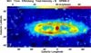 |
Fig. 1. Total intensity I (in colour) of M 31 at λ11.3 cm smoothed to 5′ HPBW, in coordinates along the major and minor axes of the ring of M 31. The rms noise is 1.0 mJy beam−1. The lines show the apparent magnetic field orientations (not corrected for Faraday rotation) at the same resolution with lengths proportional to polarized intensity PI, where the length of a beam width corresponds to 3 mJy beam−1. No lines are plotted where PI is below 1.0 mJy beam−1 or where I is negative. Background sources have been subtracted. The HPBW is indicated in the bottom left corner. |
Figure 5 shows the full field of the total emission at λ6.2 cm before subtraction of the background sources that are unrelated to M 31. These sources have been discussed before by Berkhuijsen et al. (1983).
The linearly polarized emission from M 31 (Figs. 2, 7, and 10) is also concentrated in the ring-like structure. The main differences to the distribution of total emission are the minima around the major axis of the projected ring. This shows that the ordered magnetic field in the ring is oriented almost along the line of sight on the major axis, and hence almost follows the ring (Beck 1982). The variation of polarized intensity along the ring is discussed in Sect. 7.
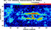 |
Fig. 2. Polarized intensity PI (in colour) of M 31 at λ11.3 cm smoothed to 5′ HPBW, in coordinates along the major and minor axes of M 31. The rms noise is 0.3 mJy beam−1. The lines show the apparent magnetic field orientations (not corrected for Faraday rotation) at the same resolution with lengths proportional to polarized intensity PI, where the length of a beam width corresponds to 3 mJy beam−1. No lines are plotted where PI is below 1.0 mJy beam−1. Polarized background sources have been subtracted. The HPBW is indicated in the bottom left corner. |
Significant polarized emission (more than 3 times the rms noise) is detected at λ11.3 cm also outside the ring of M 31 in the NE (Fig. 2). Some regions are about the same size as the telescope beam and could be weak polarized background sources. Extended polarized patches may originate in the foreground of our Milky Way. Polarized patches in the region of M 31 were also observed at λ21.1 cm (Berkhuijsen et al. 2003). They are called Faraday ghosts, and are caused by Faraday rotation and depolarization of smooth polarized emission occurring in nearby magnetized regions in the foreground. They appear only in PI, but not in total intensity I, and are especially prominent when observing at lower frequencies, for example with the WSRT at around λ90 cm (e.g. Haverkorn et al. 2003; Schnitzeler et al. 2009) or around λ2 m (150 MHz) (e.g. Iacobelli et al. 2013), or with the LOw Frequency Array (LOFAR) at around λ2 m (e.g. Jelić et al. 2015; Van Eck et al. 2017). Some of the polarized regions outside of the ring to the north-east may originate in high-velocity H I clouds belonging to M 31 that are mixed with dust seen at 250 μm (Fritz et al. 2012) (see Fig. 3).
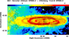 |
Fig. 3. Apparent magnetic field orientations (not corrected for Faraday rotation) of M 31 at λ11.3 cm at 5′ HPBW with lengths proportional to polarized intensity PI, overlaid onto an image of 250 μm infrared emission from Fritz et al. (2012) (arbitrary units, in log10 scale), smoothed to 2′ HPBW, indicated in the bottom left corner. The coordinate system is rotated by −53°. |
The apparent magnetic field orientations (i.e. the polarization angles +90°) in Figs. 1, 6, and 9 strongly differ for the three frequencies, demonstrating the action of Faraday rotation. The orientations of the intrinsic magnetic field (corrected for Faraday rotation) shown in Figs. 4 and 8 agree well and show that the magnetic field closely follows the ring. In Sect. 7, maps of Faraday rotation measures are discussed.
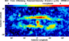 |
Fig. 4. Polarized intensity PI (in colour) of M 31 at λ11.3 cm smoothed to 5′ HPBW, in coordinates along the major and minor axes intrinsic magnetic field orientations at the same resolution, corrected for Faraday rotation measured between λ11.3 cm and λ6.2 cm (see Fig. 21), with lengths proportional to the degree of polarization, where the length of a beam width corresponds to 30%. No lines are plotted where I or PI is below 3 times the rms noise. Polarized background sources have been subtracted. The HPBW is indicated in the bottom left corner. |
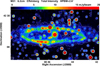 |
Fig. 5. Total intensity I (colour and contours) of M 31 at λ6.2 cm at the original HPBW of |

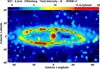 |
Fig. 6. Total intensity I (in colour) of M 31 at λ6.2 cm smoothed to 3′ HPBW, in coordinates along the major and minor axes of M 31. The rms noise is 0.35 mJy beam−1. The lines show the apparent magnetic field orientations (not corrected for Faraday rotation) at the same resolution with lengths proportional to polarized intensity PI, where the length of a beam width corresponds to 1.5 mJy beam−1. No lines are plotted where PI is below 0.3 mJy beam−1 or where I is negative. Background sources have been subtracted. The HPBW is indicated in the bottom left corner. |
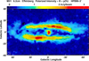 |
Fig. 7. Polarized intensity PI (in colour) of M 31 at λ6.2 cm smoothed to 3′ HPBW, in coordinates along the major and minor axes of M 31. The rms noise is 0.06 mJy beam−1. The lines show the apparent magnetic field orientations (not corrected for Faraday rotation) at the same resolution with lengths proportional to the degree of polarization, where the length of a beam width corresponds to 30%. No lines are plotted where I or PI is below 3 times the rms noise. Polarized background sources have been subtracted. The HPBW is indicated in the bottom left corner. |
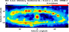 |
Fig. 8. Total non-thermal intensity (in colour) of M 31 at λ6.2 cm smoothed to 3′ HPBW, in coordinates along the major and minor axes of M 31. The rms noise is 0.35 mJy beam−1. The lines show the intrinsic magnetic field orientations at the same resolution, corrected for Faraday rotation measured between λ6.2 cm and λ3.6 cm (see Fig. 22), with lengths proportional to the degree of non-thermal polarization, where the length of a beam width corresponds to 30%. No lines are plotted where PI is below 0.2 mJy beam−1. Polarized background sources have been subtracted. The HPBW is indicated in the bottom left corner. |
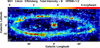 |
Fig. 9. Total intensity I (colour) of M 31 at λ3.6 cm smoothed to |

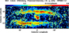 |
Fig. 10. Polarized intensity PI (colour) of M 31 at λ3.6 cm smoothed to |

The two regions of polarized emission outside the ring towards the north, detected at λ11.3 cm and λ6.2 cm, allowed us to compute the intrinsic field orientations in these areas (Fig. 4, near the left edge of the plot). These strongly deviate from the orientation of the ring and suggest a location in high-velocity clouds around M 31 or in the Milky Way foreground.
4. Spectral index
4.1. Spectral index of the integrated flux density
The galaxy M 31 has been mapped in radio continuum at more than six frequencies (see Table 3). In order to subtract the same point sources from all maps, the flux densities of the sources subtracted at 408 MHz were scaled to the frequencies of the other maps, assuming a constant spectral index of α = 0.7 (where S ∝ ν−α). These flux densities are indicated by Smin in Table 3. After subtracting sources with flux densities S > Smin, we used the data to calculate the total spectral index α of the emission integrated in three radial intervals in M 31 (i.e. R < 1 kpc, R < 5 kpc and R < 16 kpc).
Integrated flux densities of M 31 for three radial ranges for total intensity I, non-thermal intensity NTH, and thermal intensity TH.
Not all maps extend to R = 16 kpc (=70′) along the major axis. By comparing them to larger maps we estimated that in these cases about 5% of the flux density was missing and we corrected for this.
The base levels of the maps are usually set to zero in strips that are a few beam widths wide and parallel to the major axis at |b| ≈ 30′. Only the new map at λ3.6 cm does not reach that far. Therefore, we adjusted this map to the background level of the new map at λ6.2 cm at |b| ≈ 20′ (after smoothing it to HPBW = 3′) using the task bascor of the NOD2 system. For this adjustment we assumed α = 0.9 between λ6.2 cm and λ3.6 cm at |b| ≈ 20′. This resulted in an increase in the integrated flux density for R < 16 kpc of 200 mJy.
The integration was done by adding the emission in circular rings around the centre in the plane of the galaxy. The resulting flux densities in total power of the three radial intervals are given in Table 3 and are shown in Fig. 11. The low value at λ3.6 cm for R < 5 kpc indicates that, in spite of the great efforts (Sect. 2.3), the subtracted base level of the small map around the central region was still too high.
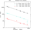 |
Fig. 11. Spectrum of the integrated flux density of total intensity I integrated to radii of 1 kpc (red), 5 kpc (cyan), and 16 kpc (black). The slopes of the fitted lines are also given in the figure. The points at λ3.6 cm were not used for the fits. |
Because of the uncertainty in the flux densities at λ3.6 cm, we calculated the spectral index between λ92 cm (0.327 GHz) and λ6.2 cm (4.85 GHz) yielding α = 0.68 ± 0.06 for R < 1 kpc, α = 0.68 ± 0.02 for R < 5 kpc, and α = 0.71 ± 0.02 for R < 16 kpc. Berkhuijsen et al. (2003) found α = 0.83 ± 0.13 for R < 16 kpc using only data at λ20.5 cm and λ6.2 cm. Within the errors their value is consistent with our value, but since our value is based on more data points and a larger frequency interval, our value of α = 0.71 ± 0.02 supersedes the old one.
In order to derive the non-thermal spectral index of the emission integrated to R < 16 kpc, we subtracted the integrated thermal emission from the total emission at each frequency, scaled from the integrated thermal emission at λ20.5 cm given by Tabatabaei et al. (2013a), using the spectral index of optically thin free-free emission of 0.1. Before scaling, we increased the value at λ20.5 cm by 5% to account for missing areas in the thermal map near the major axis. Figure 12 shows the total, non-thermal, and thermal spectra of the integrated emission. A weighted fit through the non-thermal flux densities between λ92 cm and λ6.2 cm gives the non-thermal spectral index αn = 0.81 ± 0.03. This shows that the value of αn = 1.0 between λ20.5 cm and λ6.2 cm assumed by Berkhuijsen et al. (2003) was too large, and demonstrates that spectral indices measured between only two frequencies do not always agree with that derived by fitting the data at many frequencies.
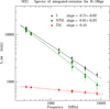 |
Fig. 12. Spectrum of the integrated flux densities of total intensity I (black), non-thermal intensity NTH (green), and thermal intensity TH (red), integrated to a radius of 16 kpc. The slopes of the fitted lines are also given in the figure. The uncertain points for I and NTH at λ3.6 cm were not used for the fits. The points for TH were scaled from the thermal map at λ20.5 cm using a slope of −0.1. |
4.2. Maps of spectral index between λ20.5 cm and λ3.6 cm
Figure 12 shows that the integrated flux densities for R < 16 kpc at λ3.6 cm agree with the extensions of the lines fitted through the points at the lower frequencies. This indicates that the base level of the map at λ3.6 cm outside the central area is correct. Therefore, we can calculate spectral index maps between λ20.5 cm (Beck et al. 1998) and λ3.6 cm of total emission (α) and non-thermal emission (αn) at the best available angular resolution of 90″ HPBW.
Before calculating spectral index maps, we subtracted from both maps the same point sources (i.e. all sources with flux densities above 5 mJy at λ20.5 cm and above 1.2 mJy at λ3.6 cm). In order to obtain maps of non-thermal emission at these frequencies, we subtracted maps of thermal emission from the maps of total emission. We used the thermal map at λ20.5 cm that Tabatabaei et al. (2013a) derived from the extinction-corrected Hα map of Devereux et al. (1994), which we smoothed to 90″ HPBW and scaled to λ3.6 cm by the factor (3.6/20.5)0.1, using the thermal spectral index of 0.1. Both I maps were cut
down to the size of the thermal map of 110′× 39′ in l × b before subtracting TH from I, and all maps were transformed onto the same grid. Figure 2 in Tabatabaei et al. (2013a) shows that due to the propagation of cosmic ray electrons (CREs) the distribution of the NTH emission is much more extended than that of the TH emission.
For the spectral index calculation, only data points above two times the noise level in both maps were used. The resulting maps of α and αn are shown in Figs. 13 and 14, respectively. We note that because of the base level problems in the innermost region 10′×10′ in size at λ3.6 cm, the spectral indices cannot be trusted there.
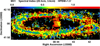 |
Fig. 13. Spectral index of the total intensity between λ20.5 cm and λ3.6 cm at |

In Fig. 13, values of α in the ring vary from about 0.4 in the middle of the ring where the H II regions are located to > 1.0 in the outer regions of the ring where most of the emission is NTH. The values of αn in Fig. 14 show the same trend as those of α, but are about 0.1 higher in the H II regions in the middle of the ring, varying between 0.5 here and > 1.0 in the outer regions. A value of αn = 0.5 near star-forming regions indicates that the CREs are still close to their birth places in the supernova remnants. Energy losses during the propagation away from their birth places cause the larger spectral indices in the outer parts of the ring.
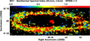 |
Fig. 14. Spectral index of the non-thermal intensity between λ20.5 cm and λ3.6 cm at |

In Figs. 13 and 14 the spectral indices are larger in the southern half of M 31 (right-hand part) than in the northern half. The α map of Berkhuijsen et al. (2003) between λ20.5 cm and λ6.2 cm shows the same trends as seen in Fig. 13, but with less detail because of the larger HPBW of 3′.
Due to the large frequency interval between λ20.5 cm and λ3.6 cm, the random noise errors in the spectral index maps are quite small, ranging from 0.013 in the middle of the ring to 0.038 in the outer parts of the ring in α (Fig. 13) and from 0.023 to 0.046 in αn (Fig. 14). The errors are dominated by the noise errors in the maps at λ3.6 cm. Systematic errors due to base level uncertainties are difficult to estimate, but could be larger than the random noise errors.
We also calculated spectral index maps between λ20.5 cm and λ6.2 cm and between λ6.2 cm and λ3.6 cm at the resolution of 3′ HPBW. They are consistent with Figs. 13 and 14, but because of the larger beam width and the narrower frequency ranges, less interesting than the higher resolution spectral index maps between λ20.5 cm and λ3.6 cm shown here. The NTH map at λ6.2 cm is shown in Fig. 8.
4.3. Radial variations in spectral index
In Fig. 15 we show the radial variation in α and αn, and the fraction of thermal emission (fth), averaged in 1 kpc wide rings between R = 6 kpc and R = 16 kpc. As discussed above, the flattest spectra occur in the middle of the ring (R = 10 − 11 kpc) where most of the H II regions are located and the TH fraction of the emission is highest. Due to the subtraction of the thermal emission, the spectrum of the NTH emission is typically steeper by about 0.1 than that of the total emission I, and both spectra become significantly steeper towards the edges of the emission ring where the NTH emission dominates. This suggests that CREs move inwards and outwards away from their birth places near star-forming regions over several kpc in radius.
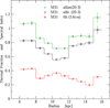 |
Fig. 15. Radial variations of the spectral index between λ20.5 cm and λ3.6 cm, of the total intensity (black), of the non-thermal intensity (green), and of the thermal fraction at λ3.6 cm (red); they are all at |

5. Radial scale lengths
It is interesting to see how the various types of emission from M 31 vary with radial distance to the galaxy centre.
In Fig. 16 we show the radial distributions of total emission and polarized emission in the new map at λ6.2 cm with angular resolution of  HPBW. The emissions were averaged in 1 kpc wide circular rings in the plane of M 31 using a constant inclination of 75°. As this map extends 140′ in longitude, the radial distribution is complete out to R = 18 kpc, beyond which some emission near the major axis is missing. The I emission from the bright ring peaks at R = 10 − 11 kpc and the PI emission at 9 kpc, then both emissions steadily decrease to about R = 20 kpc. Exponential fits for the range R = 9 − 20 kpc yield radial scale lengths of L = (3.4 ± 0.2) kpc in I and L = (4.43 ± 0.06) kpc in PI, as indicated in the figure.
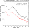 |
Fig. 16. Radial variations of total intensity I (black) and polarized intensity PI (red) at λ6.2 cm at |

The radial variations of I, NTH, TH, and PI at λ6.2 cm at 3′ HPBW are shown in Fig. 17. For the range R = 0 − 7 kpc, we used the inclinations of the H I gas increasing from 31° at R < 2 kpc to 72° at R = 6 − 7 kpc as determined by Chemin et al. (2009), assuming that the same holds for the radio continuum emission. A close correspondence between gas and radio continuum features was first pointed out by Beck (1982) and Berkhuijsen et al. (1993) and is clearly visible in Fig. 8 of Nieten et al. (2006). At larger radii we used the inclination of 75° again, which is consistent with the inclination of H I in this area. For each component we calculated the radial scale length between R = 11 kpc and R = 15 kpc, as shown in Fig. 17 and listed in Table 4. With L = (3.66 ± 0.10) kpc for NTH and L = (1.87 ± 0.05) kpc for TH, the NTH emission clearly decreases much more slowly than the TH emission, indicating propagation of the CREs away from their birth places in the star-forming regions. The scale length of PI of L = (4.84 ± 0.16) kpc is even larger than that of NTH, reflecting the large scale of the ordered magnetic field without influence of the turbulent fields of smaller scale that dominate the NTH emission.
 |
Fig. 17. Radial variations of total intensity I (black), non-thermal intensity NTH (green), thermal intensity TH (red), and polarized intensity PI (blue) at λ6.2 cm at 3′ HPBW. The exponential fits were restricted to the radial range between 11 kpc and 15 kpc. The scale lengths L are given in the figure. |
Exponential scale lengths L for the radial range 11–15 kpc at three frequencies for total intensity I, non-thermal intensity NTH, polarized intensity PI, and thermal intensity TH.
Since propagation of CREs depends on frequency, we also calculated the scale lengths at λ20.5 cm and λ3.6 cm at the angular resolution of 3′ and at the resolution of  . As before, we determined the scale lengths between 11 kpc and 15 kpc. All scale length results are given in Table 4.
Comparing the scale lengths at the resolution of 3′, we see a clear decrease in L of I and NTH with increasing frequency: L for NTH drops from (4.08 ± 0.13) kpc at λ20.5 cm to (2.79 ± 0.06) kpc at λ3.6 cm. This reflects the decrease in the propagation length of the CREs with increasing frequency and makes NTH maps at λ20.5 cm look smoother than those at λ3.6 cm. In addition, the scale length of PI decreases between λ6.2 cm and λ3.6 cm, but not as strongly as that of NTH, because PI depends on the large-scale ordered magnetic field and NTH on both the ordered and the small-scale turbulent field. Naturally, the scale length of TH is the same at each frequency.
At the resolution of  the scale lengths of I and NTH at λ20.5 cm are again larger than those at λ3.6 cm by nearly the same amount as at 3′ resolution. However, the scale lengths of I and NTH at
  are significantly smaller than those at 3′. Although at λ3.6 cm the errors are quite large, the same trend is visible and is clearest for the scale length of PI. The scale lengths are larger at 3′ resolution than at
  resolution, because of the greater smoothing of the emission at 3′ resolution than at
  resolution. At λ3.6 cm the effect is smaller than at λ20.5 cm because the propagation length at the higher frequency is smaller than at λ20.5 cm. As TH emission is least diffuse, at both frequencies the scale length of TH is only slightly smaller at
  than at 3′.
6. Azimuthal variation of polarized intensity
Polarized intensity PI is proportional to the component of the ordered (i.e. regular plus anisotropic turbulent) field perpendicular to the line of sight, Bord, ⊥. The strength of the PI depends on the strength and geometry of the ordered field, the density of the CREs, and the amount of depolarization.
Figure 18 shows the azimuthal variation of polarized intensity at λ3.6 cm and λ6.2 cm in the emission ring. Polarized intensity reveals maxima near the minor axis and minima near the major axis. Fits of a double-periodic curve give phase shifts of −9 ° ±3° at λ3.6 cm and −14 ° ±2° at λ6.2 cm, with the latter fit being statistically better. Variations in the CRE density or the strength of the ordered field are independent of the locations of the major and minor axis and cannot explain the variation seen in Fig. 18. Depolarization by Faraday dispersion in turbulent magnetic fields could in principle increase from the minor to the major axis due to the increasing path length through the emission ring. However, the emission ring between 9 kpc and 11 kpc radius is flat, with a scale height of the thermal gas of only about 0.5 kpc (Fletcher et al. 2004) compared to a radial width of about 4 kpc (Fig. 17), resulting in an almost constant path length between the minor and the major axis, which disfavours a strong variation in Faraday depolarization. Depolarization by RM gradients (Fletcher et al. 2004) is strongest near the minor axis (Fig. 24) and also cannot explain the variation in Fig. 18. Furthermore, Faraday depolarization is strongly wavelength dependent and is expected to be weak at λ3.6 cm and λ6.2 cm. In the next paper, we will discuss Faraday depolarization in detail.
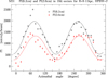 |
Fig. 18. Variation of polarized intensity PI at λ3.6 cm (red) and λ6.2 cm (black) at 3′ HPBW with azimuthal angle ϕ in the plane of M 31, averaged in 10° sectors in the ring between 9 kpc and 11 kpc radius. The azimuthal angle is counted anticlockwise from the north-eastern major axis of the ring in the plane of the sky (see Fig. 19). The lines show the weighted fits. |
We conclude that the variation in polarized intensity is due to variation in the orientation of the ordered field with respect to the line of sight. The polarized intensity is strongest around the minor axis and weakest around the major axis, which indicates that the orientation of the ordered field approximately follows the ring, as is clearly visible in Figs. 4 and 8, so that its component in the plane of the sky varies with azimuthal angle with a phase shift that is related to the spiral pitch angle ξord of the large-scale ordered field.
To investigate this geometrical effect in detail, we computed the aspect angle βord between the ordered magnetic field and the line of sight, so that Bord, ⊥ = Bord sin βord and Bord, ∥ = Bord cos βord. For a large-scale ASS pattern of the ordered field with a constant pitch angle ξord,
 (1)
(1)
where i = 75° is the galaxy inclination, and ϕ is the azimuthal angle in the galaxy plane, counted anticlockwise, with ϕ = 0° on the north-eastern and ϕ = 180° on the south-western major axis of the ring (see Fig. 19). For a constant CRE density, constant strength of the ordered field, constant path length through the emitting ring, and negligible Faraday depolarization, polarized intensity PI varies as
 (2)
(2)
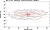 |
Fig. 19. Sectors of 20° in width in the galaxy plane (red lines) and major and minor axes (black lines), superimposed onto contours of polarized intensity PI at λ6.2 cm at 3′ HPBW. Contour levels are at (0.6, 1.2, 2.4) × 1 mJy beam−1. The azimuthal angle is counted anticlockwise from the north-eastern major axis of the ring (left side). |
where αnth is the synchrotron spectral index2. According to Eq. (2), the maxima of PI are expected at βord = 90° (i.e. at azimuthal angles of ϕ = (90 ° +ξord) and ϕ = (270 ° +ξord)), and the minima at βord = (90 ° −i) (i.e. at ϕ = +ξord and ϕ = (180 ° +ξord)).
When plotting loge(PI) against loge(sin βord), the slope of the fit should give 1 + αnth in the case of a perfect ASS field and no depolarization. Figure 20 and Table 5 show the results for four quadrants of the radial ring between 9 kpc and 11 kpc, each covering a range of azimuthal angles corresponding to a range in aspect angle between βord = (90 ° −i) and βord = 90°. Here we assumed that the ordered field has a large-scale ASS pattern with a pitch angle of ξord = −15°3. The slopes of the first three quadrants are consistent with the mean synchrotron spectral index of about 0.75 (Fig. 15). In these quadrants, the variation of PI is mostly due to the variation in aspect angle β. In the fourth quadrant (north) (ϕ = 260 ° −340°) the slope is significantly different from the expectation for the simple geometry. In this region the ordered field deviates from the assumed ASS geometry in strength and/or in orientation.
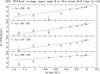 |
Fig. 20. Variation of polarized intensity PI at λ3.6 cm (in μJy beam−1, in loge scale) at |

In a similar study by Beck (1982) of PI at λ11.1 cm (Fig. 6 therein), the slopes were different from the expected value in all four quadrants, probably due to the lower resolution and significant Faraday depolarisation at that wavelength. Our new results are more consistent with the ASS field pattern.
Beck (1982) suggested that the field orientation follows gaseous spiral arms observed in H I (Unwin 1980a,b; Braun 1990; Chemin et al. 2009) that deviate from a simple ring structure. The main H I spiral arm in the north-western quadrant is almost straight from the minor axis to close to the major axis, so that β hardly varies, which may explain the small slope in Fig. 20 (bottom panel).
7. Faraday rotation and large-scale field pattern
Faraday rotation is a tool used to study the pattern of the large-scale regular field, but it is insensitive to a large-scale pattern of the anisotropic turbulent field. We computed Faraday rotation measures RM = Δχ/ (where λ is measured in metres) from the polarization angles χ between λ1 = 0.1133 m and λ2 = 0.0618 m at 5′ resolution, and also between λ1 = 0.0618 m and λ2 = 0.0359 m at 3′ resolution (Figs. 21 and 22). In both figures RM varies smoothly along the ring, with the lowest values near the north-eastern major axis and the highest near the south-western major axis. A few regions outside of the ring (near the left edge of Fig. 21) show significant deviations from this behaviour.
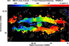 |
Fig. 21. Faraday rotation measure RM (colour) between λ11.3 cm and λ6.2 cm at 5′ HPBW, calculated at pixels where PI at both frequencies exceeds three times the rms noise. The error decreases from 26 rad m−2 at the lowest signal-to-noise ratio (S/N = 3) to about 3 rad m−2 at the highest S/N. Contours show the polarized intensity at λ11.3 cm at the same resolution. Contour levels are at 1, 2, and 4 mJy beam−1. Polarized background sources have been subtracted. The HPBW is indicated in the bottom left corner. The coordinate system is rotated by −53°. |
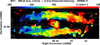 |
Fig. 22. Faraday rotation measure RM (colour) between λ6.2 cm and λ3.6 cm at 3′ HPBW, calculated at pixels where PI at both frequencies exceeds three times the rms noise. The error decreases from 93 rad m−2 at S/N = 3 to about 9 rad m−2 at the highest S/N. Contours show the polarized intensity at λ6.2 cm at the same resolution. Contour levels are at 0.5, 1, and 2 mJy beam−1. Polarized background sources have been subtracted. The HPBW is indicated in the bottom left corner. The coordinate system is rotated by −53°. |
The RMs in the central region are different in the two figures: about −150 rad m−2 in Fig. 21 and about −100 rad m−2 in Fig. 22. Gießübel & Beck (2014) measured the RM between λ6.2 cm and λ3.5 cm in the central region with 15″ resolution and found periodic variations of about ±100 rad m−2 around the foreground RMfg ≃ −100 rad m−2, which indicates a separate ASS field in the central region. The beam width of our new observations is too large to resolve this inner field.
If the large-scale ASS pattern of the ordered field found in Sect. 6 is also valid for the regular field (which is part of the ordered field), the RM is expected to vary as (see Krause et al. 1989)
 (3)
(3)
where RMfg is the RM contribution from the Milky Way in the foreground of M 31; ϕ is the azimuthal angle in the galaxy plane; βreg is the aspect angle between the regular field and the line of sight; ξreg is the pitch angle of the regular field, assumed to be constant along ϕ; and RMmax, a is the maximum RM of the ASS mode near the south-western major axis of the ring (i.e. at the azimuthal angle ϕ = 180 ° +ξreg). Figures 23 and 24 show that sinusoidal variations give good fits to the data averaged in sectors of the radial ring between 9 kpc and 11 kpc.
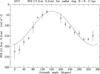 |
Fig. 23. Variation (with azimuthal angle in the galaxy plane) of Faraday rotation measures RM between λ11.3 cm and λ6.2 cm at 5′ HPBW, averaged in the radial ring between 9 kpc and 11 kpc in sectors of 20° width, and the fitted sinusoidal line. The azimuthal angle is counted from the north-eastern major axis (left side in Fig. 21). The reduced χ2 value is 4.0. |
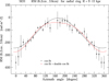 |
Fig. 24. Variation (with azimuthal angle in the galaxy plane) of Faraday rotation measures RM between λ6.2 cm and λ3.6 cm at 3′ HPBW, averaged in the radial ring between 9 kpc and 11 kpc, in sectors of 10° width. The black line shows the sinusoidal fit, the red line the combined sinusoidal + double-periodic fit, with reduced χ2 values of 1.3 for both fits. |
The foreground RMs of the sinusoidal fits in the radial ring 9–11 kpc are similar, RMfg = ( − 118 ± 3) rad m−2 between λ11.3 cm and λ6.2 cm (Fig. 23) and RMfg = ( − 125 ± 4) rad m−2 between λ6.2 cm and λ3.6 cm (Fig. 24, black curve). The amplitude RMmax,a = (78±6) rad m−2 between λ11.3 cm and λ6.2 cm is lower compared to RMmax,a = (118±9) rad m−2 between λ6.2 cm and λ3.6 cm in the same radial range by a factor of ≃1.5. As this factor characterizes the relative amount of Faraday depolarization, M 31 is less transparent to polarized emission (partly “Faraday thick”) at λ11.3 cm compared to λ6.2 cm and λ3.6 cm.
We performed sinusoidal fits according to Eq. (3) for the RM data between λ6.2 cm and λ3.6 cm for five radial rings between 7 kpc and 12 kpc in the galaxy plane. The results are given in Table 6. The average RMfg of ( − 125 ± 5) rad m−2 is smaller than the values of about −90 rad m−2 found based on previous data (Beck 1982; Berkhuijsen et al. 2003), but the new data are more reliable. The value of RMfg does not show a significant variation with radius, indicating that RMs from the Milky Way do not vary on an angular scale similar to that of the ring width in M 31. The amplitudes RMmax, a increase with radius, indicating that the strength of the regular field of M 31 increases outwards, as already noted by Fletcher et al. (2004). The pitch angles ξreg are similar to the pitch angle of the gaseous spiral arms of about −7° (Arp 1964; Braun 1991; Chemin et al. 2009).
Fit results of the sinusoidal azimuthal variation of RM between λ6.2 cm and λ3.6 cm at 3′ HPBW, averaged in sectors of 10° width, in five radial rings ΔR in the galaxy plane.
Linear models of α–Ω dynamo action in galaxies (Shukurov 2000) predict that the absolute value of the pitch angle |ξreg| is constant for a flat rotation curve, but that it decreases with increasing radius if the scale height of the gas disc increases (“flaring disc”). According to the non-linear dynamo model developed by Chamandy & Taylor (2015), the magnetic pitch angle, in the saturated state of field evolution, depends on several parameters that may vary differently with radius. Our results (Table 6) indicate that ξreg is about constant with radius, consistent with the prediction from the simple model. On the other hand, the mode analysis of multi-frequency polarization angles used by Fletcher et al. (2004) yielded larger values of ξreg between −11° and −19° in radial rings similar to those in Table 6 and a hint of a radial decrease. However, anisotropic turbulent fields (which affect polarization angles and intensities but not RMs) are neglected in the method of Fletcher et al. (2004), so that their values of ξreg are correct only if ξord ≃ ξreg.
The azimuthal RM variation in Fig. 24 shows significant deviations from the sinusoidal fit (black curve). Sofue & Beck (1987) suggested the existence of a BSS mode superimposed onto the ASS mode. The azimuthal variation of RM for a BSS field is (Krause 1990)
 (4)
(4)
where ϕ is the azimuthal angle in the galaxy plane and δ the phase, which is related to the pitch angle and the position angle of the spiral pattern in the galaxy plane.
The red curve in Fig. 24 shows the fit for the combined ASS + BSS field, for the radial range 9 − 11 kpc where the signal-to-noise ratios are highest. The amplitude of the BSS field is RMmax,b = (21±7) rad m−2, about six times smaller than the amplitude RMmax, a of the ASS mode. The fit of the combined modes is not statistically better because the BSS field is weak. We computed the residuals from the ASS fit (Fig. 25), which vary double-periodically with azimuthal angle and hence support the superimposed BSS field.
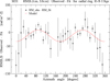 |
Fig. 25. Variation (with azimuthal angle in the galaxy plane) of the residual Faraday rotation measures RM between λ6.2 cm and λ3.6 cm at 3′ HPBW, averaged in the radial ring between 9 kpc and 11 kpc, after subtracting the best-fitting sinusoidal model from Fig. 24 (black line). The reduced χ2 value is 1.2. |
Faraday rotation allows us to compute the intrinsic pitch angle ξord of the ordered field from the observed orientation of the polarized emission in two steps, to be compared with ξreg as computed above. Firstly, the RMs shown in Figs. 21 or 22 were used to correct the orientation χobs of the ordered magnetic field in the plane of the sky observed at wavelength λ for Faraday rotation in order to achieve the intrinsic orientation (i.e. at infinitely small wavelength) in the plane of the sky via χord = χobs − RM λ2. Then the intrinsic pitch angle ξord of the ordered field in the galaxy plane follows from
![Mathematical equation: $$ \begin{aligned} \xi _\mathrm{ord} = \phi + 90\circ - \arctan \, [ \tan (\chi _\mathrm{ord} -\chi _\mathrm{p} ) / \cos \,i], \end{aligned} $$](/articles/aa/full_html/2020/01/aa36481-19/aa36481-19-eq29.gif) (5)
(5)
where χord is the intrinsic position angle of the ordered field in the plane of the sky and χp is the position angle of the major axis of the galaxy in the plane of the sky.
The azimuthal variation of the intrinsic pitch angle ξord in the ring 9–11 kpc, calculated from the intrinsic orientations of the ordered field at 3′ resolution, corrected with RMs between λ6.2 cm and λ3.6 cm, is shown in Fig. 26. The average pitch angle is −26 ° ±3° (weighted according to error bars). The average pitch angle derived from the intrinsic polarization angles at 5′ resolution, corrected with RMs between λ11.3 cm and λ6.2 cm, in the same radial range 9–11 kpc is −17 ° ±6° (also weighted according to error bars), consistent with the value obtained using the smaller wavelengths. In order to search for any radial variation, we computed averages of ξord in five radial rings, given in the last column of Table 6. No significant variation with radius is found.
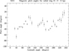 |
Fig. 26. Variation (with azimuthal angle in the galaxy plane) of the intrinsic pitch angle ξord of the ordered magnetic field, calculated from the intrinsic orientations of the ordered field at 3′ HPBW, corrected with RMs between λ6.2 cm and λ3.6 cm, and averaged in the radial ring between 9 kpc and 11 kpc. |
The large variations in the intrinsic pitch angles ξord seen in Fig. 26 indicate that the field structure is more complex than an ASS + BSS field. The value of ξord jumps by about 70° from positive to negative values near the north-eastern major axis (ϕ ≈ 0°), and ξord calculated from the intrinsic orientations of the ordered field, corrected with RMs between λ11.3 cm and λ6.2 cm, shows a similar behaviour. We propose that ξord is affected by local field deviations and/or anisotropic turbulent fields.
The averages of ξord in Table 6 are significantly smaller than those of ξreg and the pitch angle of the gaseous spiral arms of about −7°. Pitch angles of the ordered field that deviate from those of the gaseous spiral arms have also been found in the spiral galaxies M 74 (Mulcahy et al. 2017), M 83 (Frick et al. 2016), and M 101 (Berkhuijsen et al. 2016). These results were believed to show that the mean-field dynamo does not generate regular fields that are aligned with the spiral arms because ξreg depends on several parameters that are unrelated to spiral arms (Chamandy & Taylor 2015).
The results for M 31 presented here suggest a different interpretation: Bord has two components, the regular field Breg and the anisotropic turbulent field Ban. As ξreg in Table 6 is similar to the pitch angle of the gaseous spiral arms of about −7°, the deviation may arise in the anisotropic turbulent field. The regular field Breg and the anisotropic turbulent field Ban have different spiral patterns that may be shaped by different physical processes.
8. Summary and conclusions
In order to study the magnetic field structure of M 31, we used the Effelsberg telescope to perform three new deep radio continuum surveys in total intensity and polarization at the wavelengths of λ11.3 cm (2.645 GHz), λ6.2 cm (4.85 GHz), and λ3.6 cm (8.35 GHz). The angular resolutions (HPBW) are  ,
,  , and
, and  , respectively (Table 2). As we wanted to study the large-scale emission, we subtracted point sources unrelated to M 31 at each wavelength. The resulting maps are shown in Figs. 1–10.
In this first paper we have presented the observations and reduction procedures and discussed results on the spectral index and radial scale lengths, and on Faraday rotation measures and pitch angles of the regular magnetic field. Below we summarize our main conclusions:
-
At all wavelengths the well-known emission ring between about 7 kpc and 13 kpc radius in the galaxy plane stands out, both in I and in PI. The nuclear region is also very bright. PI is low on the major axis of the ring in the plane of the sky on both sides, which is a first indication that the ordered magnetic field is oriented along the bright ring, so that the field component in the plane of the sky is smallest near the major axis.
-
Including all available surveys between 0.3 GHz and 4.85 GHz, covering M 31 to at least R = 16 kpc, we find a spectral index of the integrated total emission of α = 0.71 ± 0.02 (defined as S ∝ ν−α). After subtraction of the thermal emission, we obtain a spectral index of the integrated non-thermal emission of αn = 0.81 ± 0.03.
-
The spectral indices vary across M 31. Maps of total and non-thermal spectral indices between λ21.1 cm and λ3.6 cm at
 resolution show that α (αn) is about 0.4 (0.5) near star-forming regions and steepens to about 1.0 towards the inner and outer parts of the bright ring due to radiation losses of the CREs propagating away from their birth places near the star-forming regions.
 -
The radial variation of the intensities of I, NTH, PI, and TH all peak between 8 and 12 kpc radius, but their scale lengths (L) differ. At λ6.2 cm and 3′ resolution, between R = 11 kpc and R = 15 kpc, we find L(I) = (3.02 ± 0.11) kpc, L(NTH) = (3.66 ± 0.10) kpc, L(PI) = (4.84 ± 0.16) kpc, and L(TH) = (1.87 ± 0.05) kpc. The longer scale lengths of NTH and PI than of TH again indicate energy losses of the CREs when travelling away from their birthplaces near star-forming regions. The difference in scale lengths shows that the propagation length of the CREs could be several kpc.
-
The polarized intensity, averaged in azimuthal sectors in the radial ring between 9 kpc and 11 kpc in the galaxy plane, varies with azimuthal angle as a double-periodic curve, with maxima near the minor axis and minima near the major axis. This indicates that the ordered magnetic field is oriented almost along the ring but has a small pitch angle.
-
Faraday rotation measures (RMs) between λ11.3 cm and λ6.2 cm and between λ6.2 cm and λ3.6 cm, averaged in azimuthal sectors of the radial ring between 9 kpc and 11 kpc, vary smoothly along the emission ring as a cosine function with azimuthal angle in the galaxy plane, which is a signature of a regular field with an axisymmetric spiral (ASS) pattern. The phase shift of the variation of −7 ° ±2° is interpreted as the average spiral pitch angle of the regular field. It shows no significant variation with radius and is similar to the pitch angle of the gaseous spiral arms.
-
The residuals between the RMs computed between λ6.2 cm and λ3.6 cm and the ASS fit show a double-periodic variation with azimuthal angle, indicative of a superimposed BSS mode of the regular field, with an about six times smaller amplitude compared to the ASS mode.
-
The amplitude of the RMs between λ11.3 cm and λ6.2 cm between 9 kpc and 11 kpc radius is about 1.5 times lower than between λ6.2 cm and λ3.6 cm, indicating that Faraday depolarization at λ11.3 cm is stronger (greater Faraday thickness) than at λ6.2 cm and λ3.6 cm).
-
The average pitch angle of the ordered field, derived from the intrinsic orientations of the polarized emission between 9 kpc and 11 kpc radius, is −26 ° ±3°. The difference in pitch angles of regular and ordered field indicates that the ordered field contains a significant fraction of an anisotropic turbulent field that has a pattern that is different to the regular (ASS + BSS) field.
New insights to the magnetic field of M 31, especially measuring the extent in the outer disc and the search for large-scale reversals, can be expected from deep observations of polarized background sources in L band (λ20 cm, hence improving the pioneering work performed by Han et al. (1998). While the southern location of the Square Kilometre Array (SKA, under construction) hampers observation of M 31, the Jansky Very Large Array (JVLA) and APERTIF (Oosterloo et al. 2018) are suitable instruments for such investigations.
A negative pitch angle indicates that the spiral pattern is trailing with respect to the global rotation.
Equation (2) is also valid for the case of equipartition between the energy densities of cosmic rays and total magnetic fields ( ) because Btot is dominated by small-scale turbulent fields that do not depend on βord.
While the fit to the λ6.2 cm data in Fig. 18 gave ξord = −14 ° ±2°, we decided to use a value of −15°, which gives a symmetric assignment of the azimuthal sectors to the four quadrants.
Acknowledgments
We thank the operators at the Effelsberg telescope for support during on-site observations and for supervising remote observations. We thank Patricia Reich for her support at various stages of data processing, especially for writing the turboplait script and for an early version of the script subtrans. Peter Müller is acknowledged for making several data processing scripts available to us already during the development of NOD3. We thank Marita Krause, Andrew Fletcher, and the anonymous referee for careful reading of the manuscript and useful suggestions.
References
- Arp, H. 1964, ApJ, 139, 1045 [NASA ADS] [CrossRef] [Google Scholar]
- Arshakian, T. G., & Beck, R. 2011, MNRAS, 418, 2336 [NASA ADS] [CrossRef] [Google Scholar]
- Arshakian, T. G., Beck, R., Krause, M., & Sokoloff, D. 2009, A&A, 494, 21 [NASA ADS] [CrossRef] [EDP Sciences] [Google Scholar]
- Beck, R. 1982, A&A, 106, 121 [NASA ADS] [Google Scholar]
- Beck, R. 2007, A&A, 470, 539 [NASA ADS] [CrossRef] [EDP Sciences] [Google Scholar]
- Beck, R. 2015, A&ARv, 24, 4 [NASA ADS] [CrossRef] [Google Scholar]
- Beck, R., & Golla, G. 1988, A&A, 191, L9 [NASA ADS] [Google Scholar]
- Beck, R., & Gräve, R. 1982, A&A, 105, 192 [NASA ADS] [Google Scholar]
- Beck, R., Berkhuijsen, E. M., & Wielebinski, R. 1980, Nature, 283, 272 [NASA ADS] [CrossRef] [Google Scholar]
- Beck, R., Loiseau, N., Hummel, E., et al. 1989, A&A, 222, 58 [NASA ADS] [Google Scholar]
- Beck, R., Brandenburg, A., Moss, D., Shukurov, A., & Sokoloff, D. 1996, ARA&A, 34, 155 [NASA ADS] [CrossRef] [Google Scholar]
- Beck, R., Berkhuijsen, E. M., & Hoernes, P. 1998, A&AS, 129, 329 [NASA ADS] [CrossRef] [EDP Sciences] [Google Scholar]
- Berkhuijsen, E. M. 1977, A&A, 57, 9 [NASA ADS] [Google Scholar]
- Berkhuijsen, E. M., Wielebinski, R., & Beck, R. 1983, A&A, 117, 141 [NASA ADS] [Google Scholar]
- Berkhuijsen, E. M., Bajaja, E., & Beck, R. 1993, A&A, 279, 359 [NASA ADS] [Google Scholar]
- Berkhuijsen, E. M., Beck, R., & Hoernes, P. 2003, A&A, 398, 937 [NASA ADS] [CrossRef] [EDP Sciences] [Google Scholar]
- Berkhuijsen, E. M., Beck, R., & Tabatabaei, F. S. 2013, MNRAS, 435, 1598 [NASA ADS] [CrossRef] [Google Scholar]
- Berkhuijsen, E. M., Urbanik, M., Beck, R., & Han, J. L. 2016, A&A, 588, A114 [NASA ADS] [CrossRef] [EDP Sciences] [Google Scholar]
- Boulares, A., & Cox, D. P. 1990, ApJ, 365, 544 [NASA ADS] [CrossRef] [Google Scholar]
- Brandenburg, A., & Subramanian, K. 2005, Phys. Rep., 417, 1 [NASA ADS] [CrossRef] [Google Scholar]
- Braun, R. 1990, ApJS, 72, 755 [NASA ADS] [CrossRef] [Google Scholar]
- Braun, R. 1991, ApJ, 372, 54 [NASA ADS] [CrossRef] [Google Scholar]
- Braun, R., Thilker, D. A., Walterbos, R. A. M., & Corbelli, E. 2009, ApJ, 695, 937 [Google Scholar]
- Brinks, E., & Shane, W. W. 1984, A&AS, 55, 179 [NASA ADS] [Google Scholar]
- Chamandy, L. 2016, MNRAS, 462, 4402 [NASA ADS] [CrossRef] [Google Scholar]
- Chamandy, L., & Taylor, A. R. 2015, ApJ, 808, 28 [NASA ADS] [CrossRef] [Google Scholar]
- Chemin, L., Carignan, C., & Foster, T. 2009, ApJ, 705, 1395 [NASA ADS] [CrossRef] [Google Scholar]
- de Vaucouleurs, G., de Vaucouleurs, A., & Corwin, J. R. 1976, Second Reference Catalogue of Bright Galaxies (Austin: University of Texas Press) [Google Scholar]
- Devereux, N. A., Price, R., Wells, L. A., & Duric, N. 1994, AJ, 108, 1667 [NASA ADS] [CrossRef] [Google Scholar]
- Emerson, D. T., & Gräve, R. 1988, A&A, 190, 353 [NASA ADS] [Google Scholar]
- Emerson, D. T., Klein, U., & Haslam, C. G. T. 1979, A&A, 76, 92 [NASA ADS] [Google Scholar]
- Evirgen, C. C., Gent, F. A., Shukurov, A., Fletcher, A., & Bushby, P. J. 2019, MNRAS, 488, 5065 [NASA ADS] [CrossRef] [Google Scholar]
- Fletcher, A., Berkhuijsen, E. M., Beck, R., & Shukurov, A. 2004, A&A, 414, 53 [NASA ADS] [CrossRef] [EDP Sciences] [Google Scholar]
- Frick, P., Stepanov, R., Beck, R., et al. 2016, A&A, 585, A21 [NASA ADS] [CrossRef] [EDP Sciences] [Google Scholar]
- Fritz, J., Gentile, G., Smith, M. W. L., et al. 2012, A&A, 546, A34 [NASA ADS] [CrossRef] [EDP Sciences] [Google Scholar]
- Gießübel, R. 2012, PhD Dissertation, Universität zu Köln, Cuvillier Verlag Göttingen, Germany [Google Scholar]
- Gießübel, R., & Beck, R. 2014, A&A, 571, A61 [NASA ADS] [CrossRef] [EDP Sciences] [Google Scholar]
- Gießübel, R., Heald, G., Beck, R., & Arshakian, T. G. 2013, A&A, 559, A27 [NASA ADS] [CrossRef] [EDP Sciences] [Google Scholar]
- Golla, G. 1989, Diploma Thesis, Universität zu Bonn, Germany [Google Scholar]
- Gordon, K. D., Bailin, J., Engelbracht, C. W., et al. 2006, ApJ, 638, L87 [Google Scholar]
- Han, J. L., Beck, R., & Berkhuijsen, E. M. 1998, A&A, 335, 1117 [NASA ADS] [Google Scholar]
- Hanasz, M., Wóltański, D., & Kowalik, K. 2009, ApJ, 706, L155 [NASA ADS] [CrossRef] [Google Scholar]
- Haverkorn, M., Katgert, P., & de Bruyn, A. G. 2003, A&A, 403, 1045 [NASA ADS] [CrossRef] [EDP Sciences] [Google Scholar]
- Hoernes, P., Berkhuijsen, E. M., & Xu, C. 1998, A&A, 334, 57 [NASA ADS] [Google Scholar]
- Iacobelli, M., Haverkorn, M., & Katgert, P. 2013, A&A, 549, A56 [NASA ADS] [CrossRef] [EDP Sciences] [Google Scholar]
- Jacoby, G. H., Ford, H., & Ciardullo, R. 1985, ApJ, 290, 136 [NASA ADS] [CrossRef] [Google Scholar]
- Jelić, V., de Bruyn, A. G., Pandey, V. N., et al. 2015, A&A, 583, A137 [NASA ADS] [CrossRef] [EDP Sciences] [Google Scholar]
- Kothes, R., Reich, P., Foster, T. J., & Reich, W. 2017, A&A, 597, A116 [NASA ADS] [CrossRef] [EDP Sciences] [Google Scholar]
- Krause, M. 1990, in Galactic and Intergalactic Magnetic Fields, eds. R. Beck, R. Wielebinski, & P. P. Kronberg, IAU Symp., 140, 187 [NASA ADS] [CrossRef] [Google Scholar]
- Krause, M., Hummel, E., & Beck, R. 1989, A&A, 217, 4 [NASA ADS] [Google Scholar]
- Krumholz, M. R., & Federrath, C. 2019, Front. Astron. Space Sci., 6, 7 [NASA ADS] [CrossRef] [Google Scholar]
- Melchior, A.-L., & Combes, F. 2011, A&A, 536, A52 [NASA ADS] [CrossRef] [EDP Sciences] [Google Scholar]
- Moss, D., Stepanov, R., Arshakian, T. G., et al. 2012, A&A, 537, A68 [NASA ADS] [CrossRef] [EDP Sciences] [Google Scholar]
- Mulcahy, D. D. 2011, Master Thesis, Universität zu Bonn, Germany [Google Scholar]
- Mulcahy, D. D., Beck, R., & Heald, G. H. 2017, A&A, 600, A6 [NASA ADS] [CrossRef] [EDP Sciences] [Google Scholar]
- Müller, P., Krause, M., Beck, R., & Schmidt, P. 2017a, A&A, 606, A41 [NASA ADS] [CrossRef] [EDP Sciences] [Google Scholar]
- Müller, P., Beck, R., & Krause, M. 2017b, A&A, 600, A63 [NASA ADS] [CrossRef] [EDP Sciences] [Google Scholar]
- Nieten, C., Neininger, N., Guélin, M., et al. 2006, A&A, 453, 459 [NASA ADS] [CrossRef] [EDP Sciences] [Google Scholar]
- Oosterloo, T., van Leeuwen, J., Van Cappellen, W., Kruithof, G., & Jackson, C. 2018, Westerbork Telescope 50th Anniversary, 361, 16 [Google Scholar]
- Peng, B., Kraus, A., Krichbaum, T. P., & Witzel, A. 2000, A&AS, 145, 1 [NASA ADS] [CrossRef] [EDP Sciences] [Google Scholar]
- Perley, R. A., & Butler, B. J. 2013, ApJS, 206, 16 [Google Scholar]
- Perley, R. A., & Taylor, G. B. 2003, NRAO Tech. Rep. [Google Scholar]
- Rahmani, S., Lianou, S., & Barmby, P. 2016, MNRAS, 456, 4128 [NASA ADS] [CrossRef] [Google Scholar]
- Ruzmaikin, A. A., Sokolov, D. D., & Shukurov, A. M. 1988, in Magnetic Fields of Galaxies, Astrophys. Space Sci. Lib., 133 [CrossRef] [Google Scholar]
- Ruzmaikin, A., Sokolov, D., Shukurov, A., & Beck, R. 1990, A&A, 230, 284 [NASA ADS] [Google Scholar]
- Schnitzeler, D. H. F. M., Katgert, P., & de Bruyn, A. G. 2009, A&A, 494, 611 [NASA ADS] [CrossRef] [EDP Sciences] [Google Scholar]
- Shukurov, A. 2000, in Proceedings 232. WE-Heraeus Seminar, eds. E. M. Berkhuijsen, R. Beck, & R. A. M. Walterbos, 191 [Google Scholar]
- Sieber, W., Haslam, C. G. T., & Salter, C. J. 1979, A&A, 74, 361 [NASA ADS] [Google Scholar]
- Sofue, Y., & Beck, R. 1987, PASJ, 39, 541 [NASA ADS] [Google Scholar]
- Sofue, Y., & Takano, T. 1981, PASJ, 33, 47 [NASA ADS] [Google Scholar]
- Sokoloff, D. D., Bykov, A. A., Shukurov, A., et al. 1998, MNRAS, 299, 189 [NASA ADS] [CrossRef] [Google Scholar]
- Stanek, K. Z., & Garnavich, P. M. 1998, ApJ, 503, L131 [NASA ADS] [CrossRef] [Google Scholar]
- Stepanov, R., Arshakian, T. G., Beck, R., Frick, P., & Krause, M. 2008, A&A, 480, 45 [NASA ADS] [CrossRef] [EDP Sciences] [Google Scholar]
- Tabatabaei, F. S., & Berkhuijsen, E. M. 2010, A&A, 517, A77 [NASA ADS] [CrossRef] [EDP Sciences] [Google Scholar]
- Tabatabaei, F. S., Schinnerer, E., Murphy, E. J., et al. 2013a, A&A, 552, A19 [NASA ADS] [CrossRef] [EDP Sciences] [Google Scholar]
- Tabatabaei, F. S., Berkhuijsen, E. M., Frick, P., Beck, R., & Schinnerer, E. 2013b, A&A, 557, A129 [NASA ADS] [CrossRef] [EDP Sciences] [Google Scholar]
- Unwin, S. C. 1980a, MNRAS, 190, 551 [NASA ADS] [CrossRef] [Google Scholar]
- Unwin, S. C. 1980b, MNRAS, 192, 243 [NASA ADS] [Google Scholar]
- Van Eck, C. L., Haverkorn, M., Alves, M. I. R., et al. 2017, A&A, 597, A98 [NASA ADS] [CrossRef] [EDP Sciences] [Google Scholar]
- Zweibel, E. G. 2013, Phys. Plasmas, 20, 055501 [NASA ADS] [CrossRef] [Google Scholar]
All Tables
Integrated flux densities of M 31 for three radial ranges for total intensity I, non-thermal intensity NTH, and thermal intensity TH.
Exponential scale lengths L for the radial range 11–15 kpc at three frequencies for total intensity I, non-thermal intensity NTH, polarized intensity PI, and thermal intensity TH.
Fit results of the sinusoidal azimuthal variation of RM between λ6.2 cm and λ3.6 cm at 3′ HPBW, averaged in sectors of 10° width, in five radial rings ΔR in the galaxy plane.
All Figures
|
Fig. 1. Total intensity I (in colour) of M 31 at λ11.3 cm smoothed to 5′ HPBW, in coordinates along the major and minor axes of the ring of M 31. The rms noise is 1.0 mJy beam−1. The lines show the apparent magnetic field orientations (not corrected for Faraday rotation) at the same resolution with lengths proportional to polarized intensity PI, where the length of a beam width corresponds to 3 mJy beam−1. No lines are plotted where PI is below 1.0 mJy beam−1 or where I is negative. Background sources have been subtracted. The HPBW is indicated in the bottom left corner. |
| In the text | |
|
Fig. 2. Polarized intensity PI (in colour) of M 31 at λ11.3 cm smoothed to 5′ HPBW, in coordinates along the major and minor axes of M 31. The rms noise is 0.3 mJy beam−1. The lines show the apparent magnetic field orientations (not corrected for Faraday rotation) at the same resolution with lengths proportional to polarized intensity PI, where the length of a beam width corresponds to 3 mJy beam−1. No lines are plotted where PI is below 1.0 mJy beam−1. Polarized background sources have been subtracted. The HPBW is indicated in the bottom left corner. |
| In the text | |
|
Fig. 3. Apparent magnetic field orientations (not corrected for Faraday rotation) of M 31 at λ11.3 cm at 5′ HPBW with lengths proportional to polarized intensity PI, overlaid onto an image of 250 μm infrared emission from Fritz et al. (2012) (arbitrary units, in log10 scale), smoothed to 2′ HPBW, indicated in the bottom left corner. The coordinate system is rotated by −53°. |
| In the text | |
|
Fig. 4. Polarized intensity PI (in colour) of M 31 at λ11.3 cm smoothed to 5′ HPBW, in coordinates along the major and minor axes intrinsic magnetic field orientations at the same resolution, corrected for Faraday rotation measured between λ11.3 cm and λ6.2 cm (see Fig. 21), with lengths proportional to the degree of polarization, where the length of a beam width corresponds to 30%. No lines are plotted where I or PI is below 3 times the rms noise. Polarized background sources have been subtracted. The HPBW is indicated in the bottom left corner. |
| In the text | |
|
Fig. 5. Total intensity I (colour and contours) of M 31 at λ6.2 cm at the original HPBW of |
| In the text | |
|
Fig. 6. Total intensity I (in colour) of M 31 at λ6.2 cm smoothed to 3′ HPBW, in coordinates along the major and minor axes of M 31. The rms noise is 0.35 mJy beam−1. The lines show the apparent magnetic field orientations (not corrected for Faraday rotation) at the same resolution with lengths proportional to polarized intensity PI, where the length of a beam width corresponds to 1.5 mJy beam−1. No lines are plotted where PI is below 0.3 mJy beam−1 or where I is negative. Background sources have been subtracted. The HPBW is indicated in the bottom left corner. |
| In the text | |
|
Fig. 7. Polarized intensity PI (in colour) of M 31 at λ6.2 cm smoothed to 3′ HPBW, in coordinates along the major and minor axes of M 31. The rms noise is 0.06 mJy beam−1. The lines show the apparent magnetic field orientations (not corrected for Faraday rotation) at the same resolution with lengths proportional to the degree of polarization, where the length of a beam width corresponds to 30%. No lines are plotted where I or PI is below 3 times the rms noise. Polarized background sources have been subtracted. The HPBW is indicated in the bottom left corner. |
| In the text | |
|
Fig. 8. Total non-thermal intensity (in colour) of M 31 at λ6.2 cm smoothed to 3′ HPBW, in coordinates along the major and minor axes of M 31. The rms noise is 0.35 mJy beam−1. The lines show the intrinsic magnetic field orientations at the same resolution, corrected for Faraday rotation measured between λ6.2 cm and λ3.6 cm (see Fig. 22), with lengths proportional to the degree of non-thermal polarization, where the length of a beam width corresponds to 30%. No lines are plotted where PI is below 0.2 mJy beam−1. Polarized background sources have been subtracted. The HPBW is indicated in the bottom left corner. |
| In the text | |
|
Fig. 9. Total intensity I (colour) of M 31 at λ3.6 cm smoothed to |
| In the text | |
|
Fig. 10. Polarized intensity PI (colour) of M 31 at λ3.6 cm smoothed to |
| In the text | |
|
Fig. 11. Spectrum of the integrated flux density of total intensity I integrated to radii of 1 kpc (red), 5 kpc (cyan), and 16 kpc (black). The slopes of the fitted lines are also given in the figure. The points at λ3.6 cm were not used for the fits. |
| In the text | |
|
Fig. 12. Spectrum of the integrated flux densities of total intensity I (black), non-thermal intensity NTH (green), and thermal intensity TH (red), integrated to a radius of 16 kpc. The slopes of the fitted lines are also given in the figure. The uncertain points for I and NTH at λ3.6 cm were not used for the fits. The points for TH were scaled from the thermal map at λ20.5 cm using a slope of −0.1. |
| In the text | |
|
Fig. 13. Spectral index of the total intensity between λ20.5 cm and λ3.6 cm at |
| In the text | |
|
Fig. 14. Spectral index of the non-thermal intensity between λ20.5 cm and λ3.6 cm at |
| In the text | |
|
Fig. 15. Radial variations of the spectral index between λ20.5 cm and λ3.6 cm, of the total intensity (black), of the non-thermal intensity (green), and of the thermal fraction at λ3.6 cm (red); they are all at |
| In the text | |
|
Fig. 16. Radial variations of total intensity I (black) and polarized intensity PI (red) at λ6.2 cm at |
| In the text | |
|
Fig. 17. Radial variations of total intensity I (black), non-thermal intensity NTH (green), thermal intensity TH (red), and polarized intensity PI (blue) at λ6.2 cm at 3′ HPBW. The exponential fits were restricted to the radial range between 11 kpc and 15 kpc. The scale lengths L are given in the figure. |
| In the text | |
|
Fig. 18. Variation of polarized intensity PI at λ3.6 cm (red) and λ6.2 cm (black) at 3′ HPBW with azimuthal angle ϕ in the plane of M 31, averaged in 10° sectors in the ring between 9 kpc and 11 kpc radius. The azimuthal angle is counted anticlockwise from the north-eastern major axis of the ring in the plane of the sky (see Fig. 19). The lines show the weighted fits. |
| In the text | |
|
Fig. 19. Sectors of 20° in width in the galaxy plane (red lines) and major and minor axes (black lines), superimposed onto contours of polarized intensity PI at λ6.2 cm at 3′ HPBW. Contour levels are at (0.6, 1.2, 2.4) × 1 mJy beam−1. The azimuthal angle is counted anticlockwise from the north-eastern major axis of the ring (left side). |
| In the text | |
|
Fig. 20. Variation of polarized intensity PI at λ3.6 cm (in μJy beam−1, in loge scale) at |
| In the text | |
|
Fig. 21. Faraday rotation measure RM (colour) between λ11.3 cm and λ6.2 cm at 5′ HPBW, calculated at pixels where PI at both frequencies exceeds three times the rms noise. The error decreases from 26 rad m−2 at the lowest signal-to-noise ratio (S/N = 3) to about 3 rad m−2 at the highest S/N. Contours show the polarized intensity at λ11.3 cm at the same resolution. Contour levels are at 1, 2, and 4 mJy beam−1. Polarized background sources have been subtracted. The HPBW is indicated in the bottom left corner. The coordinate system is rotated by −53°. |
| In the text | |
|
Fig. 22. Faraday rotation measure RM (colour) between λ6.2 cm and λ3.6 cm at 3′ HPBW, calculated at pixels where PI at both frequencies exceeds three times the rms noise. The error decreases from 93 rad m−2 at S/N = 3 to about 9 rad m−2 at the highest S/N. Contours show the polarized intensity at λ6.2 cm at the same resolution. Contour levels are at 0.5, 1, and 2 mJy beam−1. Polarized background sources have been subtracted. The HPBW is indicated in the bottom left corner. The coordinate system is rotated by −53°. |
| In the text | |
|
Fig. 23. Variation (with azimuthal angle in the galaxy plane) of Faraday rotation measures RM between λ11.3 cm and λ6.2 cm at 5′ HPBW, averaged in the radial ring between 9 kpc and 11 kpc in sectors of 20° width, and the fitted sinusoidal line. The azimuthal angle is counted from the north-eastern major axis (left side in Fig. 21). The reduced χ2 value is 4.0. |
| In the text | |
|
Fig. 24. Variation (with azimuthal angle in the galaxy plane) of Faraday rotation measures RM between λ6.2 cm and λ3.6 cm at 3′ HPBW, averaged in the radial ring between 9 kpc and 11 kpc, in sectors of 10° width. The black line shows the sinusoidal fit, the red line the combined sinusoidal + double-periodic fit, with reduced χ2 values of 1.3 for both fits. |
| In the text | |
|
Fig. 25. Variation (with azimuthal angle in the galaxy plane) of the residual Faraday rotation measures RM between λ6.2 cm and λ3.6 cm at 3′ HPBW, averaged in the radial ring between 9 kpc and 11 kpc, after subtracting the best-fitting sinusoidal model from Fig. 24 (black line). The reduced χ2 value is 1.2. |
| In the text | |
|
Fig. 26. Variation (with azimuthal angle in the galaxy plane) of the intrinsic pitch angle ξord of the ordered magnetic field, calculated from the intrinsic orientations of the ordered field at 3′ HPBW, corrected with RMs between λ6.2 cm and λ3.6 cm, and averaged in the radial ring between 9 kpc and 11 kpc. |
| In the text | |
Current usage metrics show cumulative count of Article Views (full-text article views including HTML views, PDF and ePub downloads, according to the available data) and Abstracts Views on Vision4Press platform.
Data correspond to usage on the plateform after 2015. The current usage metrics is available 48-96 hours after online publication and is updated daily on week days.
Initial download of the metrics may take a while.