| Issue |
A&A
Volume 632, December 2019
|
|
|---|---|---|
| Article Number | A55 | |
| Number of page(s) | 10 | |
| Section | Galactic structure, stellar clusters and populations | |
| DOI | https://doi.org/10.1051/0004-6361/201936710 | |
| Published online | 27 November 2019 | |
An outer shade of Pal: Abundance analysis of the outer halo globular cluster Palomar 13⋆
1
Zentrum für Astronomie der Universität Heidelberg, Astronomisches Rechen-Institut, Mönchhofstr. 12, 69120 Heidelberg, Germany
e-mail: This email address is being protected from spambots. You need JavaScript enabled to view it.
2
National Research Council of Canada, Herzberg Astronomy and Astrophysics Research Centre, 5071 West Saanich Road, Victoria, BC V9E 2E7, Canada
Received:
16
September
2019
Accepted:
15
October
2019
Abstract
At a Galactocentric distance of 27 kpc, Palomar 13 is an old globular cluster (GC) belonging to the outer halo. We present a chemical abundance analysis of this remote system from high-resolution spectra obtained with the Keck/HIRES spectrograph. Owing to the low signal-to-noise ratio of the data, our analysis is based on a coaddition of the spectra of 18 member stars. We are able to determine integrated abundance ratios for 16 species of 14 elements, of α-elements (Mg, Si, Ca, and Ti), Fe-peak (Sc, Mn, Cr, Ni, Cu, and Zn), and neutron-capture elements (Y and Ba). While the mean Na abundance is found to be slightly enhanced and halo-like, our method does not allow us to probe an abundance spread that would be expected in this light element if multiple populations are present in Pal 13. We find a metal-poor mean metallicity of −1.91 ± 0.05 (statistical) ±0.22 (systematic), confirming that Pal 13 is a typical metal-poor representative of the outer halo. While there are some differences between individual α-elements, such as halo-like Mg and Si versus the mildly lower Ca and Ti abundances, the mean [α/Fe] of 0.34 ± 0.06 is consistent with the marginally lower α component of the halo field and GC stars at similar metallicity. We discuss our results in the context of other objects in the outer halo and consider which of these objects were likely accreted. We also discuss the properties of their progenitors. While chemically, Pal 13 is similar to Gaia-Enceladus and some of its GCs, this is not supported by its kinematic properties within the Milky Way system. Moreover, its chemodynamical similarity with NGC 5466, a purported progeny of the Sequoia accretion event, might indicate a common origin in this progenitor. However, the ambiguities in the full abundance space of this comparison emphasize the difficulties in unequivocally labeling a single GC as an accreted object, let alone assigning it to a single progenitor.
Key words: techniques: spectroscopic / stars: abundances / Galaxy: abundances / Galaxy: evolution / Galaxy: halo / globular clusters: individual: Palomar 13
Full Table 2 is only available at the CDS via anonymous ftp to cdsarc.u-strasbg.fr (130.79.128.5) or via http://cdsarc.u-strasbg.fr/viz-bin/cat/J/A+A/632/A55
© ESO 2019
1. Introduction
The Galactic halo is a variegated place, populated by a mix of stellar populations and subsystems that likely have different origins. Our current understanding of hierarchical galaxy formation has been highly successful in identifying components that formed in situ as well as those that formed in external environments, such as stars accreted from dwarf spheroidal (dSph) galaxies (Cooper et al. 2013; Pillepich et al. 2015) or disrupted globular clusters (GCs), which have been shown to have contributed at the ∼10% level to the build-up of the stellar halo of the Milky Way (MW; Martell & Grebel 2010; Koch et al. 2019a). In turn, Kruijssen et al. (2019) and Massari et al. (2019) estimated that ∼35–40% (i.e., ∼55–65) of the present-day MW GCs are of extragalactic origin and that the main contribution to the halo up to z ∼ 2 came from three major accretion events: Sagittarius (Ibata et al. 1994; Law & Majewski 2010), Gaia-Enceladus (Belokurov et al. 2018; Helmi et al. 2018), and Sequoia (Myeong et al. 2019).
Clearly, the GCs that are currently observed to belong to the MW are important probes of the formation and evolution of the early Galaxy; in particular, the formation history of the outer halo is imprinted in these GCs, which are located at large Galactocentric distances. From a practical perspective, one of the best ways to investigate the origin of any given stellar system is to perform “chemical tagging”, a method that we employ here.
Our target, Palomar 13 (hereafter Pal 13), is a stellar system located in the outer halo, at a Galactocentric distance of 27 kpc (Siegel et al. 2001). The cluster is is currently thought to be close to apogalacticon (Küpper et al. 2011). By analyzing ages and dynamics of the Galactic GC system, Massari et al. (2019) associated Pal 13 with the Sequoia event, a metal-poor system ([Fe/H] peaking at −1.6 dex) that merged with the MW 9 Gyr ago. Côté et al. (2002) carried out a dynamical study of the cluster based on radial velocities measured from spectra with high resolution, but low signal-to-noise ratio (S/N) of candidate red giant branch (RGB) stars. They found an intrinsic velocity dispersion of 2.2 ± 0.4 km s−1, which, though modest, translates into a surprisingly high mass-to-light ratio. It is possible, however, that this value may be inflated by spectroscopic binaries (Blecha et al. 2004). Alternatively, an inflated velocity dispersion could be the result of tidal heating or shocking (Küpper et al. 2011; Yepez et al. 2019). A break in the cluster density profile has indeed been noted by some researchers, which manifests itself in a shallow outer surface density profile (Côté et al. 2002; Bradford et al. 2011; Hamren et al. 2013; Muñoz et al. 2018),
Here, we continue our efforts to obtain chemical abundance constraints of remote systems in the outer Galactic halo by performing a chemical analysis by coadding spectra of high spectral resolution but low S/N. This method was shown to be successful in our series of papers dealing with the group of Palomar clusters (Koch et al. 2009; Koch & Côté 2010, 2017; see also Koch et al. 2019b).
This paper is organized as follows. In Sect. 2 we introduce the spectroscopic sample and the observations, while Sect. 3 focuses on the radial velocity measurements and cluster membership. In Sect. 4 we describe the abundance analysis through spectrum coaddition. The respective results are presented in Sect. 5 before we discuss Pal 13 in a broader accretion context in Sect. 6. Finally, in Sect. 7 we summarize our findings.
2. Targets and observations
The data used in our work are part of the program described by Côté et al. (2002), which studied the internal dynamics of outer halo GCs. Spectra of 30 RGB candidates were taken between August 1998 and August 1999 with the High Resolution Echelle Spectrometer (HIRES) on the Keck I telescope (Vogt et al. 1994) with the C1 decker (0.86″) and 1 × 2 binning. The resulting spectral resolution is 45 000, and our spectra cover a wavelength range of 4300–6720Å.
Target stars were selected by Côté et al. (2002) from the published color-magnitude diagrams (CMDs) of Ortolani et al. (1985, herafter ORS) and their own photometry, collected with Keck and the Canada–France–Hawaii Telescope (CFHT). Details for the stars we used are listed in Table 1, and a CMD is shown in Fig. 1.
Stellar properties.
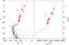 |
Fig. 1. CMD (left panel) and Kiel diagram (right panel). The member stars we used are shown as red symbols. Overlaid are metal-poor old isochrones from Bergbusch & Vandenberg (1992) using the GC parameters as shown in Fig. 4 of Côté et al. (2002). |
3. Radial velocities and membership
The radial velocity of each program star was measured by cross-correlating its spectrum against that of a master template created during each run from the observations of IAU standard stars. In order to minimize possible systematic effects, a master template for each observing run was derived from a similar and in some cases identical sample of IAU standard stars. From each cross-correlation function, we measured both vr, the heliocentric radial velocity, and RTD, the Tonry & Davis (1979) estimator of the strength of the cross-correlation peak. We followed the procedures described in Vogt et al. (1995) to derive empirical estimates for radial velocity uncertainties using the measured RTD values. The weighted radial velocities from Côté et al. (2002) are reported in Table 1. We note that additional radial velocity measurements for some of these stars have since been published by Blecha et al. (2004) and Bradford et al. (2011).
For our abundance analysis, we reduced the HIRES data in a standard manner with the Makee1 pipeline. Specifically, we used the spectra of 18 radial velocity member stars with individual S/Ns of between 3 and 16 per pixel. Star V2 was excluded from our sample due to the difficulties inherent in abundance determinations of variable RR Lyrae stars unless the ephemerides are precisely known (e.g., For et al. 2011). We also note that the member star ORS-91 is likely an asymptotic giant branch (AGB) star, judging by its position blueward of the RGB locus. Côté et al. (2002) discussed whether the stars ORS-32 and ORS-118 are members of Pal 13, based on CMD position, radial velocity, metallicity, and proper motion. The authors concluded that both these stars are probably bona fide members of Pal 13, and we therefore include them in our spectroscopic analysis.
4. Abundance analysis
The main goal in acquiring this spectroscopic data set was to study the internal dynamics of faint GCs belonging to the MW halo. Individual exposure times were accordingly short, ranging from 10 to 70 min, which leads to the low S/Ns listed in Table 1. While these S/N levels are sufficient for measuring accurate radial velocities, they are too low for meaningful chemical abundance measurements, except for the overall metallicity. Therefore, we relied on our technique of coadding all available spectra and performing a coadded abundance analysis, which we have shown in previous studies to yield reliable results (Koch et al. 2009; Koch & Côté 2010, 2017).
4.1. Stellar parameters
We started by assigning each star an effective temperature from its (B − V) colors, for which we used the calibrations of Alonso et al. (1999). These adopt an initial metallicity estimate of −2 dex, as found in previous CMD studies and a reddening of E(B − V) = 0.10 (Schlafly & Finkbeiner 2011). The typical uncertainty due to photometric and calibration errors on Teff is ∼100 K.
The surface gravities were subsequently computed using the standard stellar structure equations (e.g., Eq. (1) in Koch & McWilliam 2008). These use the above temperatures, a distance to Pal 13 of 26.9 kpc, an initial metallicity estimate of −2 dex (which enters through the bolometric correction that we adopted from the Kurucz grids), and masses of 0.8 and 0.6 M⊙ for RGB and AGB stars, respectively. We note, however, that the mass choice for the AGB star has no effect on the final abundance results because its contribution to the coadded spectrum (i.e., one of 18 stars) is negligible. The errors on all input values are propagated through the formalism, which yields a typical uncertainty on log g of 0.2 dex.
Microturbulence was fixed from the same empirical calibration of ξ with Teff that we obtained in our previous studies from the metal-poor halo sample of Roederer et al. (2014). This relation reads 4.567 − 6.2694 × 10⁻⁴ × Teff. The uncertainty on microturbulence is determined from the scatter about this above relation and amounts to 0.10 km s−1. All resulting stellar parameters for our stellar atmospheres are listed in Table 1 and are summarized in the Kiel diagram of Figs. 1 and 2.
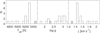 |
Fig. 2. Distribution of stellar parameters for the 18 target stars. Clear bars are for the RGB stars, and the solid bar indicates the AGB star. |
4.2. Coadded abundance measurements
As in our previous studies, we began by median-combining the spectra of the 18 stars after weighting them by their S/Ns, which facilitates the σ clipping within the IRAF program scombine. This results in an enhanced S/N of 33 per pixel at 6600 Å, which is sufficient for a detailed element abundance study. On this composite spectrum, equivalent widths (EWs) were measured using the line lists from our previous studies, which in turn are based on Koch et al. (2016) and Ruchti et al. (2016). In practice, we employed the IRAF task splot to fit Gaussian profiles to the individual lines. These line lists and EW measurements are reported in Table 2.
Line list.
Throughout our analysis, we used the stellar abundance code MOOG (Sneden 1973). Stellar atmospheres for every star were computed from the ATLAS grid of Kurucz one-dimensional 72-layer, plane-parallel, line-blanketed models without convective overshoot. In this analysis, we assumed that local thermodynamic equilibrium (LTE) holds for all species, and we used the α-enhanced opacity distribution functions AODFNEW, which is expected to hold for metal-poor halo objects.
Next, we computed theoretical EWs for all all measured transitions using the ewfind option of MOOG. These were combined into a mean ⟨EW⟩ following the identical weighting scheme as for the observed spectra (Eq. (1) in Koch & Côté 2010). Finally, the abundance ratios of the elements in question were varied so as to match the coadded ⟨EW⟩ with the observed ones to deliver the integrated element abundance.
4.3. Abundance errors
For our error analysis, we employed a standard procedure. To this end, we state the statistical error in terms of its 1σ line-to-line scatter and N, the number of lines used to measure every element abundance. For Na, Si, and Sc, only one line could be measured in each case. For Zn, we were able to measure two features that yielded a very low 1σ scatter of lower than 0.01 dex, however. In these cases, we varied the measured EWs by ±5 mÅ, corresponding to ∼20%, as a realistic uncertainty in our splot procedure. This yielded typical uncertainties of between 0.11 and 0.18 dex for the Na, Si, Sc, and Zn abundance ratios, respectively.
In addition, we varied each stellar parameter by its representative uncertainty (Teff ± 200 K; log g ± 0.2 dex; ξ ± 0.1 km s−1) and redetermined abundances through our coaddition scheme. We also accounted for an uncertainty in the α enhancement when we switched to the solar-scaled opacity distribution functions ODFNEW. This procedure yielded the systematic errors reported in Table 3 in terms of the deviation of the abundances from the altered atmospheres from those based on the original parameter set.
Systematic uncertainties.
As in past studies, we note that our approach assumes that all stars that enter the coaddition are subjected to identical errors. We also assumed that they share the same direction of deviations from the unchanged values. We further caution that the total systematic errors that we obtained by a simple quadratic sum of all contributions neglects the covariances between the stellar parameters, predominantly between temperature and gravity, and, by our empirical scaling, the microturbulence. Thus, the values listed in Table 3 should be taken as conservative upper limits.
Additional error sources such as radial velocity shifts, potential foreground contaminants, and erroneous stellar type assignments were thoroughly discussed by Koch & Côté (2010). We reiterate that these effects account for less than ∼0.05 dex in the final error budget.
5. Abundance results
All abundance results and the errors as described in Sect. 4.3 are listed in Table 4. These are placed into context with the MW halo, bulge, disks, and MW GCs with a purported accretion origin in Figs. 3 through 5. The sources for the GC abundance data are referenced in Table 5, and their implications are further discussed in Sect. 6.
Abundance results from coadded spectra.
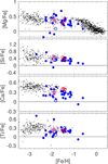 |
Fig. 3. Abundance results for the α-elements. Literature data for the MW (black dots) are as follows: for the halo, Roederer et al. (2014); for the bulge, Johnson et al. (2012, 2014); and for the disks, Bensby et al. (2014). Pal 13 is shown as the orchid star, where the error bar accounts for both statistical and systematic uncertainties. Blue filled points indicate the abundances of the comparison GCs (see Table 5 for references), while open blue symbols denote outer halo GCs beyond 20 kpc that have not been uniquely assigned to a specific progenitor. We also show as red circles the results from our systematic coadded abundance study of outer halo GCs (Koch et al. 2009; Koch & Côté 2010, 2017). |
5.1. Iron abundance and metallicity
We find a mean iron abundance from the neutral lines of −1.91 ± 0.05 (stat.) ±0.22 (sys.) dex and an excellent ionization balance of [Fe I/II] = −0.01 ± 0.12. The latter was not necessarily fulfilled in our previous coadded abundance analyses of remote GCs, and the sense of the departure of Fe I from Fe II was also found to vary from case to case (e.g., Koch et al. 2009 vs. Koch & Côté 2010). This implies that reaching ionization equilibrium is not a generic outcome of our method, but rather depends on the quality of the adopted gravities and input (stellar) parameters.
Older literature values for the metallicity of Pal 13 from Strömgren photometry and low-resolution spectra range from −1.67 to −1.90 (Canterna & Schommer 1978; Friel et al. 1982; Zinn & Diaz 1982). This was later refined by Côté et al. (2002), who coadded spectra of one star from the present sample (ORM-118) and measured an [Fe/H] of −1.98 ± 0.31 from 28 Fe lines, but at a lower S/N than our present study. All these estimates are in excellent agreement within the errors with our high-resolution spectroscopic abundance. We note, however, that the recent CMD study of Hamren et al. (2013) and a low-resolution spectroscopic analysis of 16 member stars by Bradford et al. (2011) indicate a more moderate metallicity of −1.6 ± 0.1 dex, which is marginally consistent with our result if we account for the full statistical and systematic errors.
5.2. Light elements (Na)
Sodium is the only light element for which an abundance ratio could be obtained, and this result is only based on one detected line. One of the key features of interest in GCs is the presence of light-element variations and (anti-) correlations (Carretta et al. 2009; Bastian & Lardo 2018) due to the presence of multiple stellar populations. Unfortunately, none of the other participating elements (O and Al) could be measured so that our data cannot probe the respective internal processes in Pal 13. Furthermore, as shown in Koch & Côté (2017), a coadded abundance analysis is highly insensitive to information of intrinsic abundance spreads or correlations (cf. Bastian et al. 2019). We therefore do not pursue the otherwise regular halo-like [Na/Fe] of 0.17 dex any further.
5.3. α-elements (Mg, Si, Ca, and Ti)
Manganese and silicon follow the canonical trend seen in metal-poor field and GC stars in that they lie directly at the plateau value of ∼0.4 dex. In contrast, Ca and Ti take on values that are slightly lower than the halo mean, at [Ca,Ti/Fe] = 0.29 and 0.24 dex, respectively. It is worth noting that a very good ionization balance is also reached for Ti, at [Ti I/II] = −0.03 ± 0.10. We investigate in Sect. 6 the mild depletions in these abundances in the context of the purported accretion origins of low-α GCs in more detail.
Owing to their production during different phases of the SNe II (e.g., Kobayashi et al. 2006), such as the hydrostatic burning in the progenitor (O, Mg), the explosion itself (Ca, Si), or an α-rich freeze-out (Ti), the individual α-elements are not expected to uniquely trace one another. Here, we note that the various ratio combinations of [α1/α2] show values of about −0.15 to 0.10 dex in Pal 13, which are fully representative across the halo GCs that we use for reference purposes in Sect. 6 (see also Fig. 5 in Koch & McWilliam 2011).
For simplicity, and bearing in mind the caveats of different origins, we chose to combine all four α-elements into a single abundance ratio. In doing so, we find a mean value of [α/F1e] = 0.34 ± 0.06 dex for Pal 13.
5.4. Fe-peak elements (Sc, Cr, Mn, Ni, and Zn)
Our results for the Fe-peak elements are shown in Fig. 4. We note that none of our own results was corrected for departures from LTE given the range in stellar parameters in the coadded analysis method. During our spectral coaddition, differing non-LTE (NLTE) corrections would be smeared out (but at a level that is considerably lower than our quoted uncertainties). Furthermore, the largest corrections would arise chiefly for Cr (Bergemann & Cescutti 2010), while the remainder of the elements differ only slightly (Bergemann & Gehren 2008; Korotin et al. 2018). None of these results holds any surprises, and the abundances of Pal 13 are consistent with those in halo stars and GCs at similar metallicity. The majority of abundance ratios are consistent with solar or marginally subsolar values. Mn is slightly enhanced relative to typical halo and GC stars, but considering the uncertainty of 0.25 dex, we do not see an indication for any unusual Mn production in Pal 13. While the [Cu/Fe] ratio is depleted with respect to the solar value, this is still compatible with the low[Cu/Fe] branch occupied by halo stars.
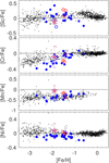 |
Fig. 4. Same as Fig. 3, but for Fe-peak elements. Here, Sc and Mn abundances for the disk are from Battistini & Bensby (2015) and Sobeck et al. (2006), while Zn abundances for the bulge are taken from Barbuy et al. (2015). |
5.5. n-capture elements (Y and Ba)
The neutron-capture elements Y and Ba in Pal 13 are slightly subsolar (Fig. 5) and closely trace the underlying Galactic halo component. We note, however, that the Y abundance is based on only two detected lines that show a sizeable 1σ dispersion. In the very metal-poor regime, the main source of the heavy elements is the r-process (Qian & Wasserburg 2007), although s-process signatures are seen as early as [Fe/H] = −2.6 (Simmerer et al. 2004). In particular, stars in dSph galaxies below −1.8 dex show systematically low [Y/Fe] abundances and consequently high [Ba/Y] ratios (Venn et al. 2004; Tolstoy et al. 2009). This was interpreted as an indication that the r-process production for Y in dSphs operates at a different site from that for Ba (Pritzl et al. 2005). At [Ba/Y] = −0.1 dex, the [h/l] ratio (e.g., Cristallo et al. 2011) in Pal 13 is mildly depleted, but it can still be considered typical of metal-poor halo and GC stars. Pritzl et al. (2005) noted that in comparison with thick disk objects as well, halo GCs tend to lie toward higher [Ba/Y] ratio, similar to stars in dSphs. While this holds true for a handful of halo objects at metallicities around −2 dex, Pal 13 does not exhibit such an offset.
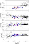 |
Fig. 5. Same as Fig. 3, but for heavy and neutron-capture elements. Data for Cu across the MW are from Mishenina et al. (2002, 2011) and Johnson et al. (2014). |
6. Is Pal 13 an accreted object?
The abundance of Pal 13 appears to be inconspicuous and very similar to the halo field and other metal-poor GCs. Often, lower α-abundances are taken as a sign of an accretion origin, although the presence of light-element (such as Mg) variations can partly veil this picture (e.g., Pritzl et al. 2005; Carretta et al. 2017). In Pal 13, a mild depletion is seen in Ca and Ti, and from this point of view, we cannot unambiguously exclude an accretion origin for these elements. However, the overall [α/Fe] and the halo-like, enhanced Mg render any such evidence only marginal. How can we then establish from the abundances whether Pal 13 is an accreted object and even conclude on the type of progenitor? This reasoning precludes that the GCs follow the mean abundance of the underlying (Galactic or extra-Galactic) component, which is indeed observed (e.g., Hendricks et al. 2016). The situation is clearer for GCs that are associated with more complex systems such as the massive Sgr dSph stream system with its very broad metallicity distribution and spatial gradients (Chou et al. 2007; Monaco et al. 2007; Hyde et al. 2015; Hansen et al. 2018).
6.1. GC comparison sample
The MW has evidently experienced at least three major accretion events that donated a major part of the stellar halo and also transferred their GC systems. The three the most recently identified accretion events (through ages and/or chemodynamics) are the disrupting Sgr dSph, the Sequoia event, and Gaia-Enceladus2.
Massari et al. (2019) combined the kinematics and ages for 151 GCs and asserted that 40% were formed in situ, 19% stem from Gaia-Enceladus, and 5–6% each originate in Sgr, Sequoia, and the Helmi streams (Helmi & White 1999; Koppelman et al. 2019). Massari et al. (2019) further separated subsamples of GCs into “main disk/bulge”, that is, objects that are not associated with accretion events, but rather with the standard underlying MW components. Furthermore, these authors identified objects with high- and low-energy orbits that have no apparent accretion origin (“unassociated”). These “regular” and presumably in situ GCs are ignored in our following reasoning. Furthermore, some of the MW GCs could not be unambiguously assigned to a single accretion event but are instead based on ages and kinematics. They share similar properties with several progenitors. Thus, for our following comparison, we are left with 18 GCs that are unequivocally associated with the Gaia-Enceladus event, 7 from Sgr, one from the Helmi streams, and four from Sequoia, for which abundances are available in the literature. Finally, we added 3 GCs that lie beyond 20 kpc from the literature. Detailed chemistry has been measured for these GCs, but according to Massari et al. (2019), they are not part of any of the substructures discussed above. These are NGC 5634 (RGC = 21 kpc; Carretta et al. 2017), NGC 5694 (RGC = 29 kpc; Mucciarelli et al. 2013), and Pal 14 (RGC = 72 kpc; Çalışkan et al. 2012).
6.2. Chemical tagging of Pal 13 and accreted GCs
In Fig. 6 we plot the [α/Fe] (bottom panels) and [Mg/Fe] (top panels) for the GCs for which abundance information is available. These ratios are representative tracers of a potential accretion origin. We differentiate these into the three progenitor groups described above (Sect. 6.1) following the association scheme of Massari et al. (2019), and those at large distances without a unique progenitor. Details and references for the chemical abundances we used in this comparison are given in Table 5.
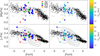 |
Fig. 6. Mg and α-element ratios for Galactic stars, Pal 13 (star), and the GCs listed in Table 5, based on Massari et al. (2019). Left panel: the clusters are color-coded by their purported origin. Right panels: same data, but color-coded by (logarithmic) Galactocentric distance, maintaining the same symbols for the different progenitors. Contours in the [α/Fe] diagrams show the Gaia-Enceladus stellar component from Helmi et al. (2018) in terms of number densities from 0.5 to 3σ in steps of 0.5σ. |
Other tracers of chemical evolution should, in the long run, also be employed to differentiate various progenitor groups and to characterize the GC-donating systems. One fo these diagnostics is the [Ba/Y] ratio, which is known to differ between halo and dSph stars (Pritzl et al. 2005, see also Sect. 5.5). However, heavy-element abundances are not known for a great number of reference GCs, and only one out of the four Sequoia-GCs has published [Ba/Y] abundance ratios. The same holds for the stellar component of these merger events, and future surveys and data releases, for example, of GALAH, are imperative to fill in this gap (Buder et al. 2018).
There is a caveat worth pointing out in this exercise: taking the mean abundance ratios as representative for the entire GC may not be appropriate for systems that have large abundance variations, or bimodalities to the point of spreading over more than 1 dex, as is the case for Mg in NGC 2419. Likewise, several abundance groups are found in NGC 7089 (Yong et al. 2014). Moreover, it is also not evident that all α-elements should be grouped into a single, straight average given their origin in different stages of the supernovae (SN) II (Venn et al. 2004; Kobayashi et al. 2006).
6.2.1. Sagittarius?
As the left panels of Fig. 6 indicate, the GCs associated with Sgr are scattered broadly in their metallicity, from below −2 up to about −0.7 dex. This rather reflects the complex metallicity distribution of the entire Sgr system: as the most massive dSph satellite still visible in the MW system today, it exhibits a broad age and metallicity range, including a very metal-poor stellar component (Hansen et al. 2018). The association of the GC with Sgr is mainly based on ages and kinematics, but two to three metal-poor GCs stand out in that they have significantly lower [α/Fe] ratios: NGC 5824 and Pal 12. Of the Sgr candidates, only Arp 2 shares the fairly regular α-abundances at the metallicity of Pal 13. We note that both GCs are located at fairly similar Galactocentric distances of 21 and 27 kpc, respectively.
Interestingly, NGC 5634 (at the same metallicity as Pal 13, [Fe/H] = −1.9) has been tagged by Massari et al. (2019) as either a Helmi stream or a Gaia-Enceladus-based object, while Law & Majewski (2010) added it to their list of Sagittarius clusters.
6.2.2. Gaia-Enceladus?
Both the stellar content of Gaia-Enceladus (shown as contours in the bottom panels of Fig. 6) and its associated GCs scatter broadly in abundance space. In this regard, finding a single object such as Pal 13 in the locus occupied by this event is expected. This event contains both GCs with very low and very high α ratios, and the full range in between is covered. If GCs do uniquely follow the underlying field component, then they should show a large overall scatter, or a well-defined knee in the [α/Fe]. The existence of low-α stars at low metallicities indicates low star formation efficiencies in the host system, leading to a (mass-dependent) early downturn in [α/Fe] caused by the onset of the Fe-producing SNe Ia (Matteucci & Brocato 1990; Tolstoy et al. 2009). If low-α stars are found at both low and high metallicities, this then appears to indicate a strongly varying star-forming efficiency and gradients across the progenitor’s main body, and if they exist, tidal streams. The location of the α knee is now recognized to be dependent not only on galaxy mass, but also on the location within the galaxy (Hendricks et al. 2014).
When we compare the entire chemical abundance pattern of Pal 13 with the named reference GCs, the closest match (in a χ2 sense) is found for NGC 6205 (M13). At first glance, this seems surprising because the object is more metal rich by 0.4 dex. Similarly, when we confine the comparison to the α elements alone among the Gaia-Enceladus GCs, then NGC 5897 provides the closest match. These similarities are, however, not consistent with the age and kinematical assignment of Pal 13 (Massari et al. 2019) and do not provide firm evidence of a connection between Pal 13 and Gaia-Enceladus.
6.2.3. Sequoia?
Based on their age and dynamical arguments, Massari et al. (2019) placed Pal 13 into the group with an origin in Sequoia, an object that was accreted 9 Gyr ago (Myeong et al. 2019), that is, at a time when Pal 13 was already some 3 Gyr old. Chemically, the Sequoia GCs do stand out, but they instead occupy a narrow metallicity window around −2 to −1.55 dex; their α enhancements reach from mild depletions around 0.2 to overenhancements of about 0.5 dex (or 0.7 in Mg).
Within the errors, Pal 13 resembles the most metal-poor progeny of Sequoia, NGC 5466. Intriguingly, Lamb et al. (2015) stated that they chose this object for abundance analysis in order to probe element trends that could establish a link with the Sgr system. However, at its low metallicity ([Fe/H] = −2), the authors did not detect any obvious differences from the Galactic halo abundance patterns. This emphasizes the difficulties in uniquely tracing the origin of a system such as Pal 13 in a given merger event based on chemistry alone (see also Reina-Campos 2019).
Finally, we show in Fig. 7 the mean α enhancement of this sample of reference GCs as a function of Galactocentric distance (see also the right panels of Fig. 6; cf. Mackey & Gilmore 2004). Here, the ratios in the Sgr GCs cover a broad range; that is, there is essentially no dependence on distance, as shown by the Pearson r value of −0.18. Although not convincingly significant, it is still worth noticing that the correlation between [α/Fe] and RGC is most pronounced for the Sequoia clusters (at r = −0.40), followed by the Gaia-Enceladus system with r = −0.35. The latter, however, strongly depends on the two GCs with a strong α enhancement (NGC 2298 and 6341, the latter being the most metal-poor GC in the MW halo).
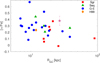 |
Fig. 7. Distance dependence of the [α/Fe] in the potentially accreted reference GCs. |
We also note that the majority of Sequoia GCs are currently at large Galactocentric distances in excess of 10 kpc, while those from Gaia-Enceladus cover a range from ∼7 to 38 kpc, 40% of which lie within 10 kpc. This may support the greater mass of this system, which caused it to perpetrate deeper into the young MW halo.
7. Summary and conclusions
We have performed a coadded chemical abundance analysis of the outer halo GC Palomar 13 and found that the majority of its abundance patterns is highly regular. In the past, some unusual properties of this object (i.e., a higher than expected velocity dispersion and unusual surface density profile) have prompted suggestions that it has experienced tidal heating. However, we found only few discernible peculiarities in chemical abundance space, although this might be expected given that its chemical patterns were likely established prior to any heating (see also Koch & Côté 2017).
Of higher importance is the question whether Pal 13 and other similar objects in the outer halo have an in or ex situ origin. Kruijssen et al. (2019) and Massari et al. (2019) estimated that ∼40% of the known MW GCs (i.e., ∼60 objects) have an extragalactic origin. For some of these halo objects, the evidence is compelling that they have been accreted: that is, those that show clear chemical signatures reminiscent of dSph galaxies or dynamical pairings with known accretion events. Other cases are less clear because they coincide with the main chemical abundance space occupied by Galactic halo stars. Chemically, Pal 13 belongs to the latter class. It has been suggested that it originated in the Sequoia event 9 Gyr ago, and both its age and orbit support this conjecture. Its abundance ratios are very similar to those of NGC 5466, which has also been identified with Sequoia. On the other hand, the latter object is equally consistent with the MW halo distribution, and unambiguous evidence for an accretion origin of either (outer) halo GC has not yet emerged.
MAKEE was developed by T. A. Barlow specifically for reduction of Keck HIRES data. It is freely available on the World Wide Web at the Keck Observatory home page, https://www2.keck.hawaii.edu/inst/common/makeewww
The latter two have by now been identified with previously detected Galactic features, the nature of which had been disputed in the past. In this vein, Gaia-Enceladus (also known as the Gaia sausage; Belokurov et al. 2018) can be identified with the Canis Major feature of the outer disk (Momany et al. 2006), whereas Sequoia poses the observational evidence for the Kraken event postulated by Kruijssen et al. (2019).
Acknowledgments
A.K. acknowledges financial support by the Deutsche Forschungsgemeinschaft (DFG, German Research Foundation) – Project-ID 138713538 – SFB 881 (“The Milky Way System”, subprojects A03, A05, A08). The authors are grateful to the anonymous referee for a swift report and to J. M. D. Kruijssen for helpful discussions. This work was based on observations obtained at the W. M. Keck Observatory, which is operated jointly by the California Institute of Technology and the University of California. We are grateful to the W. M. Keck Foundation for their vision and generosity. We recognize the great importance of Mauna Kea to both the native Hawaiian and astronomical communities, and we are grateful for the opportunity to observe from this special place.
References
- Alonso, A., Arribas, S., & Martínez-Roger, C. 1999, A&AS, 140, 261 [NASA ADS] [CrossRef] [EDP Sciences] [Google Scholar]
- Barbuy, B., Friaça, A. C. S., da Silveira, C. R., et al. 2015, A&A, 580, A40 [NASA ADS] [CrossRef] [EDP Sciences] [Google Scholar]
- Bastian, N., & Lardo, C. 2018, ARA&A, 56, 83 [NASA ADS] [CrossRef] [Google Scholar]
- Bastian, N., Usher, C., Kamann, S., et al. 2019, MNRAS, 489, L80 [NASA ADS] [Google Scholar]
- Battistini, C., & Bensby, T. 2015, A&A, 577, A9 [NASA ADS] [CrossRef] [EDP Sciences] [Google Scholar]
- Belokurov, V., Erkal, D., Evans, N. W., Koposov, S. E., & Deason, A. J. 2018, MNRAS, 478, 611 [NASA ADS] [CrossRef] [Google Scholar]
- Bensby, T., Feltzing, S., & Oey, M. S. 2014, A&A, 562, A71 [NASA ADS] [CrossRef] [EDP Sciences] [Google Scholar]
- Bergbusch, P. A., & Vandenberg, D. A. 1992, ApJS, 81, 163 [NASA ADS] [CrossRef] [Google Scholar]
- Bergemann, M., & Cescutti, G. 2010, A&A, 522, A9 [NASA ADS] [CrossRef] [EDP Sciences] [Google Scholar]
- Bergemann, M., & Gehren, T. 2008, A&A, 492, 823 [NASA ADS] [CrossRef] [EDP Sciences] [Google Scholar]
- Blecha, A., Meylan, G., North, P., & Royer, F. 2004, A&A, 419, 533 [NASA ADS] [CrossRef] [EDP Sciences] [Google Scholar]
- Bradford, J. D., Geha, M., Muñoz, R. R., et al. 2011, ApJ, 743, 167 [NASA ADS] [CrossRef] [Google Scholar]
- Buder, S., Asplund, M., Duong, L., et al. 2018, MNRAS, 478, 4513 [NASA ADS] [CrossRef] [Google Scholar]
- Çalışkan, Ş., Christlieb, N., & Grebel, E. K. 2012, A&A, 537, A83 [NASA ADS] [CrossRef] [EDP Sciences] [Google Scholar]
- Canterna, R., & Schommer, R. A. 1978, ApJ, 219, L119 [NASA ADS] [CrossRef] [Google Scholar]
- Carretta, E., Bragaglia, A., Gratton, R., & Lucatello, S. 2009, A&A, 505, 139 [NASA ADS] [CrossRef] [EDP Sciences] [Google Scholar]
- Carretta, E., Lucatello, S., Gratton, R. G., Bragaglia, A., & D’Orazi, V. 2011, A&A, 533, A69 [NASA ADS] [CrossRef] [EDP Sciences] [Google Scholar]
- Carretta, E., Bragaglia, A., Gratton, R. G., et al. 2013, A&A, 557, A138 [NASA ADS] [CrossRef] [EDP Sciences] [Google Scholar]
- Carretta, E., Bragaglia, A., Gratton, R. G., et al. 2014, A&A, 561, A87 [NASA ADS] [CrossRef] [EDP Sciences] [Google Scholar]
- Carretta, E., Bragaglia, A., Lucatello, S., et al. 2017, A&A, 600, A118 [NASA ADS] [CrossRef] [EDP Sciences] [Google Scholar]
- Chou, M.-Y., Majewski, S. R., Cunha, K., et al. 2007, ApJ, 670, 346 [NASA ADS] [CrossRef] [Google Scholar]
- Cohen, J. G. 2004, AJ, 127, 1545 [NASA ADS] [CrossRef] [Google Scholar]
- Cohen, J. G., & Kirby, E. N. 2012, ApJ, 760, 86 [NASA ADS] [CrossRef] [Google Scholar]
- Cohen, J. G., & Meléndez, J. 2005a, AJ, 129, 303 [NASA ADS] [CrossRef] [Google Scholar]
- Cohen, J. G., & Melendez, J. 2005b, AJ, 129, 1607 [NASA ADS] [CrossRef] [Google Scholar]
- Cooper, A. P., D’Souza, R., Kauffmann, G., et al. 2013, MNRAS, 434, 3348 [NASA ADS] [CrossRef] [Google Scholar]
- Côté, P., Djorgovski, S. G., Meylan, G., Castro, S., & McCarthy, J. K. 2002, ApJ, 574, 783 [NASA ADS] [CrossRef] [Google Scholar]
- Cristallo, S., Piersanti, L., Straniero, O., et al. 2011, ApJS, 197, 17 [NASA ADS] [CrossRef] [Google Scholar]
- Dalessandro, E., Lardo, C., Cadelano, M., et al. 2018, A&A, 618, A131 [NASA ADS] [CrossRef] [EDP Sciences] [Google Scholar]
- Filler, D., Ivans, I. I., & Simmerer, J. 2012, American Astronomical Society Meeting Abstracts, #219, 152.05 [NASA ADS] [Google Scholar]
- For, B.-Q., Sneden, C., & Preston, G. W. 2011, ApJS, 197, 29 [NASA ADS] [CrossRef] [Google Scholar]
- Francois, P. 1991, A&A, 247, 56 [NASA ADS] [Google Scholar]
- Friel, E., Kraft, R. P., Suntzeff, N. B., & Carbon, D. F. 1982, PASP, 94, 873 [NASA ADS] [CrossRef] [Google Scholar]
- Hamren, K. M., Smith, G. H., Guhathakurta, P., et al. 2013, AJ, 146, 116 [NASA ADS] [CrossRef] [Google Scholar]
- Hansen, C. J., El-Souri, M., Monaco, L., et al. 2018, ApJ, 855, 83 [NASA ADS] [CrossRef] [Google Scholar]
- Helmi, A., & White, S. D. M. 1999, MNRAS, 307, 495 [NASA ADS] [CrossRef] [Google Scholar]
- Helmi, A., Babusiaux, C., Koppelman, H. H., et al. 2018, Nature, 563, 85 [NASA ADS] [CrossRef] [Google Scholar]
- Hendricks, B., Koch, A., Lanfranchi, G. A., et al. 2014, ApJ, 785, 102 [NASA ADS] [CrossRef] [Google Scholar]
- Hendricks, B., Boeche, C., Johnson, C. I., et al. 2016, A&A, 585, A86 [NASA ADS] [CrossRef] [EDP Sciences] [Google Scholar]
- Hyde, E. A., Keller, S., Zucker, D. B., et al. 2015, ApJ, 805, 189 [NASA ADS] [CrossRef] [Google Scholar]
- Ibata, R. A., Gilmore, G., & Irwin, M. J. 1994, Nature, 370, 194 [NASA ADS] [CrossRef] [Google Scholar]
- Johnson, C. I., Rich, R. M., Kobayashi, C., & Fulbright, J. P. 2012, ApJ, 749, 175 [NASA ADS] [CrossRef] [Google Scholar]
- Johnson, C. I., Rich, R. M., Kobayashi, C., Kunder, A., & Koch, A. 2014, AJ, 148, 67 [NASA ADS] [CrossRef] [Google Scholar]
- Johnson, C. I., Caldwell, N., Rich, R. M., & Walker, M. G. 2017, AJ, 154, 155 [NASA ADS] [CrossRef] [Google Scholar]
- Kacharov, N., Koch, A., & McWilliam, A. 2013, A&A, 554, A81 [NASA ADS] [CrossRef] [EDP Sciences] [Google Scholar]
- Khamidullina, D. A., Sharina, M. E., Shimansky, V. V., & Davoust, E. 2014, Astrophys. Bull., 69, 409 [NASA ADS] [CrossRef] [Google Scholar]
- Kobayashi, C., Umeda, H., Nomoto, K., Tominaga, N., & Ohkubo, T. 2006, ApJ, 653, 1145 [NASA ADS] [CrossRef] [Google Scholar]
- Koch, A., & Côté, P. 2010, A&A, 517, A59 [NASA ADS] [CrossRef] [EDP Sciences] [Google Scholar]
- Koch, A., & Côté, P. 2017, A&A, 601, A41 [NASA ADS] [CrossRef] [EDP Sciences] [Google Scholar]
- Koch, A., & McWilliam, A. 2008, AJ, 135, 1551 [NASA ADS] [CrossRef] [Google Scholar]
- Koch, A., & McWilliam, A. 2011, AJ, 142, 63 [NASA ADS] [CrossRef] [Google Scholar]
- Koch, A., & McWilliam, A. 2014, A&A, 565, A23 [NASA ADS] [CrossRef] [EDP Sciences] [Google Scholar]
- Koch, A., Côté, P., & McWilliam, A. 2009, A&A, 506, 729 [NASA ADS] [CrossRef] [EDP Sciences] [Google Scholar]
- Koch, A., McWilliam, A., Preston, G. W., & Thompson, I. B. 2016, A&A, 587, A124 [Google Scholar]
- Koch, A., Grebel, E. K., & Martell, S. L. 2019a, A&A, 625, A75 [NASA ADS] [CrossRef] [EDP Sciences] [Google Scholar]
- Koch, A., Xi, S., & Rich, R. 2019b, A&A, 627, A70 [NASA ADS] [CrossRef] [EDP Sciences] [Google Scholar]
- Koppelman, H. H., Helmi, A., Massari, D., Roelenga, S., & Bastian, U. 2019, A&A, 625, A5 [NASA ADS] [CrossRef] [EDP Sciences] [Google Scholar]
- Korotin, S. A., Andrievsky, S. M., & Zhukova, A. V. 2018, MNRAS, 480, 965 [NASA ADS] [CrossRef] [Google Scholar]
- Kraft, R. P., Sneden, C., Smith, G. H., Shetrone, M. D., & Fulbright, J. 1998, AJ, 115, 1500 [NASA ADS] [CrossRef] [Google Scholar]
- Kruijssen, J. M. D., Pfeffer, J. L., Reina-Campos, M., Crain, R. A., & Bastian, N. 2019, MNRAS, 486, 3180 [NASA ADS] [CrossRef] [Google Scholar]
- Küpper, A. H. W., Mieske, S., & Kroupa, P. 2011, MNRAS, 413, 863 [NASA ADS] [CrossRef] [Google Scholar]
- Lamb, M. P., Venn, K. A., Shetrone, M. D., Sakari, C. M., & Pritzl, B. J. 2015, MNRAS, 448, 42 [NASA ADS] [CrossRef] [Google Scholar]
- Law, D. R., & Majewski, S. R. 2010, ApJ, 718, 1128 [NASA ADS] [CrossRef] [Google Scholar]
- Lovisi, L., Mucciarelli, A., Lanzoni, B., et al. 2013, ApJ, 772, 148 [NASA ADS] [CrossRef] [Google Scholar]
- Mackey, A. D., & Gilmore, G. F. 2004, MNRAS, 355, 504 [NASA ADS] [CrossRef] [MathSciNet] [Google Scholar]
- Marino, A. F., Milone, A. P., Yong, D., et al. 2017, ApJ, 843, 66 [NASA ADS] [CrossRef] [Google Scholar]
- Martell, S. L., & Grebel, E. K. 2010, A&A, 519, A14 [NASA ADS] [CrossRef] [EDP Sciences] [Google Scholar]
- Massari, D., Koppelman, H. H., & Helmi, A. 2019, A&A, 630, L4 [NASA ADS] [CrossRef] [EDP Sciences] [Google Scholar]
- Matteucci, F., & Brocato, E. 1990, ApJ, 365, 539 [NASA ADS] [CrossRef] [Google Scholar]
- McWilliam, A., Geisler, D., & Rich, R. M. 1992, PASP, 104, 1193 [NASA ADS] [CrossRef] [Google Scholar]
- Mishenina, T. V., Kovtyukh, V. V., Soubiran, C., Travaglio, C., & Busso, M. 2002, A&A, 396, 189 [NASA ADS] [CrossRef] [EDP Sciences] [Google Scholar]
- Mishenina, T. V., Gorbaneva, T. I., Basak, N. Y., Soubiran, C., & Kovtyukh, V. V. 2011, Astron. Rep., 55, 689 [Google Scholar]
- Momany, Y., Zaggia, S., Gilmore, G., et al. 2006, A&A, 451, 515 [NASA ADS] [CrossRef] [EDP Sciences] [Google Scholar]
- Monaco, L., Bellazzini, M., Bonifacio, P., et al. 2007, A&A, 464, 201 [NASA ADS] [CrossRef] [EDP Sciences] [Google Scholar]
- Mottini, M., Wallerstein, G., & McWilliam, A. 2008, AJ, 136, 614 [NASA ADS] [CrossRef] [Google Scholar]
- Mucciarelli, A., Bellazzini, M., Catelan, M., et al. 2013, MNRAS, 435, 3667 [NASA ADS] [CrossRef] [Google Scholar]
- Muñoz, R. R., Côté, P., Santana, F. A., et al. 2018, ApJ, 860, 66 [NASA ADS] [CrossRef] [Google Scholar]
- Myeong, G. C., Vasiliev, E., Iorio, G., Evans, N. W., & Belokurov, V. 2019, MNRAS, 488, 1235 [NASA ADS] [CrossRef] [Google Scholar]
- Ortolani, S., Rosino, L., & Sandage, A. 1985, AJ, 90, 473 [NASA ADS] [CrossRef] [Google Scholar]
- Pillepich, A., Madau, P., & Mayer, L. 2015, ApJ, 799, 184 [NASA ADS] [CrossRef] [Google Scholar]
- Pritzl, B. J., Venn, K. A., & Irwin, M. 2005, AJ, 130, 2140 [NASA ADS] [CrossRef] [Google Scholar]
- Qian, Y.-Z., & Wasserburg, G. J. 2007, Phys. Rep., 442, 237 [NASA ADS] [CrossRef] [Google Scholar]
- Reina-Campos, M. 2019, ArXiv eprints [arXiv:1908.00353] [Google Scholar]
- Roederer, I. U., & Sneden, C. 2011, AJ, 142, 22 [NASA ADS] [CrossRef] [Google Scholar]
- Roederer, I. U., & Thompson, I. B. 2015, MNRAS, 449, 3889 [NASA ADS] [CrossRef] [Google Scholar]
- Roederer, I. U., Preston, G. W., Thompson, I. B., et al. 2014, AJ, 147, 136 [NASA ADS] [CrossRef] [Google Scholar]
- Roederer, I. U., Mateo, M., Bailey, J. I., et al. 2016, MNRAS, 455, 2417 [NASA ADS] [CrossRef] [Google Scholar]
- Ruchti, G. R., Feltzing, S., Lind, K., et al. 2016, MNRAS, 461, 2174 [NASA ADS] [CrossRef] [Google Scholar]
- Sbordone, L., Bonifacio, P., Buonanno, R., et al. 2007, A&A, 465, 815 [NASA ADS] [CrossRef] [EDP Sciences] [Google Scholar]
- Schlafly, E. F., & Finkbeiner, D. P. 2011, ApJ, 737, 103 [NASA ADS] [CrossRef] [Google Scholar]
- Shetrone, M. D., & Keane, M. J. 2000, AJ, 119, 840 [NASA ADS] [CrossRef] [Google Scholar]
- Siegel, M. H., Majewski, S. R., Cudworth, K. M., & Takamiya, M. 2001, AJ, 121, 935 [NASA ADS] [CrossRef] [Google Scholar]
- Simmerer, J., Sneden, C., Cowan, J. J., et al. 2004, ApJ, 617, 1091 [NASA ADS] [CrossRef] [Google Scholar]
- Sneden, C. A. 1973, Ph. D. Thesis, The University of Texas at Austin, USA [Google Scholar]
- Sobeck, J. S., Ivans, I. I., Simmerer, J. A., et al. 2006, AJ, 131, 2949 [NASA ADS] [CrossRef] [Google Scholar]
- Tolstoy, E., Hill, V., & Tosi, M. 2009, ARA&A, 47, 371 [NASA ADS] [CrossRef] [Google Scholar]
- Tonry, J., & Davis, M. 1979, AJ, 84, 1511 [NASA ADS] [CrossRef] [Google Scholar]
- Venn, K. A., Irwin, M., Shetrone, M. D., et al. 2004, AJ, 128, 1177 [NASA ADS] [CrossRef] [Google Scholar]
- Villanova, S., Monaco, L., Geisler, D., et al. 2019, ApJ, 882, 174 [NASA ADS] [CrossRef] [Google Scholar]
- Vogt, S. S., Allen, S. L., Bigelow, B. C., et al. 1994, in Instrumentation in Astronomy VIII, eds. D. L. Crawford, & E. R. Craine, SPIE Conf. Ser., 2198, 362 [NASA ADS] [CrossRef] [Google Scholar]
- Vogt, S. S., Mateo, M., Olszewski, E. W., & Keane, M. J. 1995, AJ, 109, 151 [NASA ADS] [CrossRef] [Google Scholar]
- Yepez, M. A., Arellano Ferro, A., Schröder, K. P., et al. 2019, New A, 71, 1 [Google Scholar]
- Yong, D., Roederer, I. U., Grundahl, F., et al. 2014, MNRAS, 441, 3396 [NASA ADS] [CrossRef] [Google Scholar]
- Zinn, R., & Diaz, A. I. 1982, AJ, 87, 1190 [NASA ADS] [CrossRef] [Google Scholar]
All Tables
All Figures
|
Fig. 1. CMD (left panel) and Kiel diagram (right panel). The member stars we used are shown as red symbols. Overlaid are metal-poor old isochrones from Bergbusch & Vandenberg (1992) using the GC parameters as shown in Fig. 4 of Côté et al. (2002). |
| In the text | |
|
Fig. 2. Distribution of stellar parameters for the 18 target stars. Clear bars are for the RGB stars, and the solid bar indicates the AGB star. |
| In the text | |
|
Fig. 3. Abundance results for the α-elements. Literature data for the MW (black dots) are as follows: for the halo, Roederer et al. (2014); for the bulge, Johnson et al. (2012, 2014); and for the disks, Bensby et al. (2014). Pal 13 is shown as the orchid star, where the error bar accounts for both statistical and systematic uncertainties. Blue filled points indicate the abundances of the comparison GCs (see Table 5 for references), while open blue symbols denote outer halo GCs beyond 20 kpc that have not been uniquely assigned to a specific progenitor. We also show as red circles the results from our systematic coadded abundance study of outer halo GCs (Koch et al. 2009; Koch & Côté 2010, 2017). |
| In the text | |
|
Fig. 4. Same as Fig. 3, but for Fe-peak elements. Here, Sc and Mn abundances for the disk are from Battistini & Bensby (2015) and Sobeck et al. (2006), while Zn abundances for the bulge are taken from Barbuy et al. (2015). |
| In the text | |
|
Fig. 5. Same as Fig. 3, but for heavy and neutron-capture elements. Data for Cu across the MW are from Mishenina et al. (2002, 2011) and Johnson et al. (2014). |
| In the text | |
|
Fig. 6. Mg and α-element ratios for Galactic stars, Pal 13 (star), and the GCs listed in Table 5, based on Massari et al. (2019). Left panel: the clusters are color-coded by their purported origin. Right panels: same data, but color-coded by (logarithmic) Galactocentric distance, maintaining the same symbols for the different progenitors. Contours in the [α/Fe] diagrams show the Gaia-Enceladus stellar component from Helmi et al. (2018) in terms of number densities from 0.5 to 3σ in steps of 0.5σ. |
| In the text | |
|
Fig. 7. Distance dependence of the [α/Fe] in the potentially accreted reference GCs. |
| In the text | |
Current usage metrics show cumulative count of Article Views (full-text article views including HTML views, PDF and ePub downloads, according to the available data) and Abstracts Views on Vision4Press platform.
Data correspond to usage on the plateform after 2015. The current usage metrics is available 48-96 hours after online publication and is updated daily on week days.
Initial download of the metrics may take a while.