| Issue |
A&A
Volume 632, December 2019
|
|
|---|---|---|
| Article Number | A127 | |
| Number of page(s) | 13 | |
| Section | Extragalactic astronomy | |
| DOI | https://doi.org/10.1051/0004-6361/201936559 | |
| Published online | 16 December 2019 | |
The volumetric star formation law in the Milky Way
1
Dipartimento di Fisica e Astronomia, Università di Bologna, Via P. Gobetti 93/2, 40129 Bologna, Italy
e-mail: This email address is being protected from spambots. You need JavaScript enabled to view it.
2
Kapteyn Astronomical Institute, University of Groningen, Postbus 800, 9700 Groningen, The Netherlands
3
INAF – Osservatorio di Astrofisica e Scienza dello Spazio di Bologna, Via Gobetti 93/3, 40129 Bologna, Italy
4
Department of Physics, ETH Zurich, Wolfgang-Pauli-Strasse 27, 8093 Zurich, Switzerland
5
ASTRON, Netherlands Institute for Radio Astronomy, Oude Hoogeveensedijk 4, 7991 Dwingeloo, The Netherlands
6
Institute of Astronomy, University of Cambridge, Madingley Road, Cambridge CB3 0HA, UK
Received:
23
August
2019
Accepted:
5
November
2019
Abstract
Several open questions on galaxy formation and evolution have their roots in the lack of a universal star formation law that could univocally link the gas properties, such as its density, to the star formation rate (SFR) density. In a recent paper we used a sample of nearby disc galaxies to infer the volumetric star formation (VSF) law, a tight correlation between the gas and the SFR volume densities derived under the assumption of hydrostatic equilibrium for the gas disc. However, due to the dearth of information about the vertical distribution of the SFR in these galaxies, we could not find a unique slope for the VSF law, but two alternative values. In this paper, we use the scale height of the SFR density distribution in our Galaxy adopting classical Cepheids (age ≲200 Myr) as tracers of star formation. We show that this latter is fully compatible with the flaring scale height expected from gas in hydrostatic equilibrium. These scale heights allowed us to convert the observed surface densities of gas and SFR into the corresponding volume densities. Our results indicate that the VSF law ρSFR ∝ ραgas with α ≈ 2 is valid in the Milky Way as well as in nearby disc galaxies.
Key words: stars: formation / ISM: structure / galaxies: star formation / Galaxy: structure / Galaxy: disk
© ESO 2019
1. Introduction
Sixty years ago, Schmidt (1959) theorised the first star formation law for the Milky Way (MW): a power-law linking the star formation rate (SFR) and the atomic gas volume densities  . He estimated 2 < n < 3 from the HI and young stars distributions in our Galaxy. To date, much effort has gone into finding a universal relation between gas and SFR densities among all types of star-forming galaxies. We could divide the star formation laws proposed in the literature into three main groups, according to the physical quantities and scales considered.
The so-called global Schmidt–Kennicutt (SK) law involves the surface densities of gas (HI+H2; Σgas) and SFR (ΣSFR) averaged over the whole star-forming disc. This correlation was proposed by Kennicutt (1998) using a sample of regularly star-forming disc galaxies and starbursts, and it reads  with N ≈ 1.4. Recently, Kennicutt & Evans (2012) showed that the MW is compatible with the integrated SK law, while low surface brightness galaxies depart from the relation (see also de los Reyes & Kennicutt 2019).
For spatially resolved galaxies, it is possible to derive the resolved SK law (e.g. Kennicutt 1989; Martin & Kennicutt 2001), which involves the gas and the SFR surface densities measured either in kiloparsec or sub-kiloparsec regions, or their radial profiles (i.e. azimuthal averages). However, like its integrated version, this correlation seems to break in low-density environments, as found by several authors in dwarf galaxies and the outskirts of spirals (e.g. Kennicutt et al. 2007; Bolatto et al. 2011; Dessauges-Zavadsky et al. 2014). This is often ascribed to a drop in the star formation efficiency at a threshold density of about 10 M⊙ pc−2 (e.g. Schaye 2004; Leroy et al. 2008; Bigiel et al. 2008, 2010); however, the physical explanation for this behaviour is still a matter of debate (e.g. Krumholz 2014 and references therein). In our Galaxy, it is unclear whether the index of the resolved SK law is 1.4 (e.g. Fraternali & Tomassetti 2012) or higher (Wong & Blitz 2002; Boissier et al. 2003; Misiriotis et al. 2006), which may be an indication of the presence of the break (Sofue 2017).
Given that stars are thought to form from cold and dense gas, the SFR surface density is expected to correlate with the molecular gas surface density, following some molecular star formation law. This correlation is observed in high gas density regions of spiral galaxies, although its index has not been firmly established yet. Some authors find a linear correlation (e.g. Bigiel et al. 2008; Schruba et al. 2011; Marasco et al. 2012), while others derive an index around 1.4 (e.g. Wong & Blitz 2002; Heyer et al. 2004; Kennicutt et al. 2007; Liu et al. 2011). In our Galaxy, Luna et al. (2006) has investigated the molecular SK law using the SFR density traced by the far-infrared emission (i.e. dust heated by massive young stars), finding a power-law with index of 1.2 ± 0.2. However, Kennicutt & Evans (2012) shows that the H2 surface density drops faster with radius than the SFR distribution derived using HII regions (Misiriotis et al. 2006; Sofue 2017). Moving to much smaller spatial scales, Lada et al. (2010) find a linear correlation between the number of young stellar objects in Galactic molecular clouds and the mass of dense gas above an extinction threshold of 0.8 mag in K band, corresponding to about 116 M⊙ pc−2. The origin of this correlation is unclear, as it could be a consequence of the scaling relation between mass and size of molecular clouds (Lada et al. 2013).
In our previous paper (Bacchini et al. 2019, hereafter B19), we proposed a new volumetric star formation (VSF) law, a tight correlation between the SFR and the gas (HI+H2) volume densities derived for a sample of 12 nearby star-forming galaxies. The conversion of the observed surface densities into volume densities requires the knowledge of the gas and SFR scale heights. In particular, the scale heights of the HI and H2 components were computed assuming the vertical hydrostatic equilibrium in the galactic potential. A key feature of this approach is that it takes into account radial variations of the gas scale height (also called flaring) and the consequent non-linear conversion between the observed surface density and the intrinsic volume density (see also Elmegreen 2015, 2018). In the absence of observational measurements of the radial variation of the SFR vertical distribution, we decided to make two extreme assumptions for the SFR scale height. The first consisted in assuming a constant value for the entire disc (and the same for all galaxies), while the second was based on the idea that the SFR scale height is proportional to that of the most abundant gas phase, whether atomic or molecular. Clearly, these definitions for the SFR scale height led to two different radial profiles for the SFR volume density. In both cases we found a tight power-law relation, but with different indexes, 1.34 ± 0.03 and 1.91 ± 0.03.
In this work we show that the issue regarding the SFR scale height can be overcome in the MW, where the 3D structure of the tracers of recent star formation can be directly retrieved from observations, and we assess the validity of the VSF law in our Galaxy. Section 2 describes the model of the gas distribution and defines the volume densities. Section 3 presents the measurements of the distributions of gas and SFR that we took from the literature. Our results are presented in Sect. 4 and discussed in Sect. 5. Finally, in Sect. 6 we summarise the work and draw our main conclusions.
2. Volume densities
In this paper, we apply to the MW the same approach proposed in B19 for external galaxies, with the exception of the SFR scale height. For the sake of clarity, we briefly summarise the adopted methods in the following.
2.1. Distribution of gas in hydrostatic equilibrium
We assume that the HI and H2 discs are in vertical hydrostatic equilibrium in the total gravitational potential, which consists of a dark matter halo, a stellar bulge, a thin and a thick stellar disc, plus the contribution of the gas self-gravity. In general, for a given gravitational potential and gas density profile, it is possible to calculate the scale height of the gaseous component once its velocity dispersion (σ) is known, assuming that the pressure is P = ρσ2. The density distribution can be written as
![Mathematical equation: $$ \begin{aligned} \rho _i(R,z) = \rho _i(R,0) \exp \left[ - \frac{\Phi (R,z)-\Phi (R,0)}{\sigma _i^2} \right] , \end{aligned} $$](/articles/aa/full_html/2019/12/aa36559-19/aa36559-19-eq4.gif) (1)
(1)
where i stands for HI or H2, ρi(R, 0) is the volume density in the midplane, and Φ is the total gravitational potential.
We calculate the scale height via numerical integration using the software GALPYNAMICS1 (Iorio 2018), which uses an iterative algorithm to account for the gas self-gravity. In pratice, the code first calculates the external potential plus the contribution of a razor-thin gas distribution from a given parametric mass model. A first guess of the scale height is estimated by fitting a Gaussian profile (e.g. Olling 1995; Koyama & Ostriker 2009) to the gas distribution resulting from Eq. (1). The scale height (h) is defined as the standard deviation of this profile. Then Φ is updated with the potential of the new gas distribution, which includes the scale height found in the previous step, and a second estimate of the scale height is obtained by the Gaussian fitting. This procedure is iterated until two successive calculations differ by less than a given tolerance factor.
Therefore, the necessary ingredients to calculate the scale heights of HI and H2 are their surface densities and velocity dispersions (see Sect. 3.1), and a parametric mass model of the Galaxy components. In particular, we adopted the models for the stellar and dark matter distributions by McMillan (2011, 2017), which take into account observational requirements on the kinematics of gas, stars, and masers, and on the total mass of the Galaxy out to 50 kpc.
2.2. Definitions of volume densities
We define the gas volume density in the Galaxy midplane as
 (2)
(2)
where ρHI(R, 0) and ρH2(R, 0) are the volume densities of HI and H2 in the midplane, and ΣHI(R) and ΣH2(R) are the corresponding radial profiles of the surface densities. The last equality in Eq. (2) holds under the assumption of a Gaussian vertical profile for HI and H2, and hHI and hH2 are the standard deviations of these profiles. These latter were calculated using the procedure described in Sect. 2.1 based on the assumption of hydrostatic equilibrium.
We assume that the SFR is distributed in a disc with surface density ΣSFR(R) and scale height hSFR(R). Hence, the volume density of SFR in the miplane is
 (3)
(3)
The main difference with respect to B19 is that in this work we measured hSFR(R) from observations.
3. Data
3.1. Gas distribution and kinematics in the Milky Way
Several works in the literature studied the gas distribution (i.e. its surface density, volume density, and scale height) in our Galaxy adopting the kinematic distance method (Westerhout 1957). This latter relies on an assumed model of the Galactic rotation curve to transform the line-of-sight velocity into a distance from the solar position. The derived distances can then be used to obtain a full 3D reconstruction of the gas component. This method has been successfully and widely employed to map the gas densities in the entire Galaxy, but it is affected by the so-called near–far problem within the solar circle (e.g. Burton 1974; Marasco et al. 2017): the same line-of-sight velocity can be associated with two opposite distances, one between the observer and the tangent point, defined as the location where the line of sight is perpendicular to R, and one beyond it.
For this work we decided to derive the volume densities from the surface densities in the literature using the scale height calculated with the hydrostatic equilibrium. This approach allows us to compare, in a consistent way, the VSF law in the MW with that obtained in B19. In Appendix A we discuss the difference between the volume density and the scale heights estimated in the literature and those derived using the hydrostatic equilibrium.
3.1.1. Inside the solar circle
Marasco et al. (2017) studied the distribution and kinematics of the gas inside the solar circle through a novel approach that models the observed emission of HI and CO, overcoming the near–far problem. They assumed that the gas is in circular motion and divided the Galaxy in concentric and co-planar rings described by rotation velocity, velocity dispersion, scale height, and miplane volume density. Then they used a Bayesian method to fit these four parameters to the HI and the CO line emission from the Leiden-Argentine-Bonn survey (Kalberla et al. 2005) and the CO(J = 1 → 0) survey of Dame et al. (2001). This model also takes into account the extra-planar gas contribution, which was included as an additional HI component with both radial and vertical infall motions, and a lagging rotational velocity with respect to the HI in the midplane2 (see Marasco & Fraternali 2011). Their best-fit model can reproduce in detail the gas distribution and kinematics of the receding and approaching quadrants of the Galaxy. However, the assumption of pure circular orbits does not hold in the innermost 3 kpc, where the bar gravitational potential makes the gas distribution non-axisymmetric and induces non-circular motions (Binney et al. 1991; Sormani & Magorrian 2015; Sormani et al. 2015; Armillotta et al. 2019). We excluded the region R < 3 kpc in this work as our model also assumes axisymmetry. The profiles of the surface density, the volume density, and the scale height provided by Marasco et al. (2017) show three peaks that could be related to the intersection of the line of sight with spiral arms, where the density is above the mean value. Therefore, we smoothed all the profiles, including those of the velocity dispersion, from a resolution of 0.2–1.0 kpc (see Appendix A.1).
3.1.2. Beyond the solar circle
We derived an averaged profile for ΣHI from the measurements by Binney & Merrifield (1998), Nakanishi & Sofue (2003), and Levine et al. (2006), who all used the kinematic distance method, but assumed slightly different Galactic rotation curves3. For example, Levine et al. (2006) aimed to study the warp of the HI disc, which is present beyond R ∼ 12 kpc, and thus assumed that the Galaxy circular speed is constant at 220 km s−1 for R > R⊙. On the other hand, Nakanishi & Sofue (2003) adopted the rotation curve from Dehnen & Binney (1998), which slightly decreases beyond R⊙. These profiles of ΣHI are approximately in agreement with the profile by Marasco et al. (2017) in the solar vicinity (see Appendix A.1). Similarly, we used the profiles from Binney & Merrifield (1998) and Nakanishi & Sofue (2006) to calculate ΣH2.
Concerning the HI and H2 velocity dispersion, there are no available measurements of their profiles beyond R⊙, at least to our knowledge. However, several authors (e.g. Fraternali et al. 2002; Boomsma et al. 2008; Tamburro et al. 2009; Bacchini et al. 2019) have shown that in nearby spiral galaxies σHI decreases with radius until it reaches values of about 8 km s−1 and then remains roughly constant, in agreement with the outermost measurements (i.e. at R⊙) by Marasco et al. (2017). These latter also estimated σHI/σH2 ≈ 0.5 within R⊙, thus we decided to assign σHI = 8 ± 2 km s−1 and σH2 = 4 ± 1 km s−1 to all radii beyond R⊙, which are typical values for the atomic and the molecular phases (see Kramer & Randall 2016 and references therein).
3.2. SFR distribution in the MW
The SFR of our Galaxy can be estimated using different tracers of recent star formation. Chomiuk & Povich (2011) found that different measurements of the global SFR are consistent with 1.9 ± 0.4 M⊙ yr−1, if rescaled to the Kroupa initial mass function (Kroupa & Weidner 2003) and stellar population models.
3.2.1. SFR surface density
We took as reference the work by Green (2015), who carefully collected a sample of 69 bright supernova remnants (SNRs)4 in order to avoid strong selection effects. He derived the radial distribution of SNRs and found that it is more concentrated towards the Galactic centre with respect to the previous estimate by Case & Bhattacharya (1998). We derived ΣSFR(R) by normalising the radial profile of SNR surface density to the total SFR of the MW. In Appendix B.1, we show that the resulting ΣSFR(R) is compatible with other estimates obtained with different tracers and methods, albeit with a large scatter.
3.2.2. SFR scale height
To reliably measure hSFR(R), we must select a tracer of recent star formation with accurate distance determination and a sample that is statistically significant. Therefore, we chose classical Cepheids (CCs), which are variable stars typically younger than ∼200 Myr (e.g. Bono et al. 2005; Dékány et al. 2019) whose distance can be accurately determined thanks to the period-luminosity relation (e.g. Leavitt & Pickering 1912; Caputo et al. 2000; Ripepi et al. 2019). We note that SNRs and CCs are not perfectly coeval (age gap 50–100 Myr), but the dynamical processes that could modify the distribution of a population of stars with respect to the parent gas (e.g. radial migration) are effective on timescales much longer than this age gap (Sellwood 2014). Moreover, the stellar discs of star-forming galaxies grow in radius (inside-out growth) of ∼3% in 1 Gyr (Muñoz-Mateos et al. 2011; Pezzulli et al. 2015). Hence, we expect that both SNRs and CCs represent the parent gas distribution (see also Fig. B.1 for a comparison between tracers of different ages).
In a recent paper, Chen et al. (2019) collected data for 1339 CCs with distance accuracy of 3–5% from the Wide-field Infrared Survey Explorer catalogue of periodic variables and from the Gaia Data Release 2 in order to study the warp of the Galactic disc. They found that the warp seen in the distribution of CCs is compatible with that determined using pulsars (Yusifov & Küçük 2004) and atomic gas (Levine et al. 2006). After subtracting the warp contribution, these authors found evidence of a flare in the z-distribution of CCs compatible with that traced by red giant stars (Wang et al. 2018) and HI (Wouterloot et al. 1990) in the MW (see Appendix A.2).
We studied the radial profile of the scale height using the residual z-coordinates (i.e. with the warp removed) of the CCs provided by Chen et al. (2019) (see Appendix B.2 for details). Figure 1 shows the scale height of CCs: we clearly see that there is a flaring. In particular, the scale height is 100 pc at the solar position and increases with radius, reaching about 500 pc at R ≈ 18 kpc. This is a strong indication that the flaring SFR distribution is more realistic than that with a constant thickness, allowing us to disentangle between the two approaches adopted in B19 and choose the flaring hSFR(R) instead of the constant value. In Appendix B.2, the scale height of CCs is compared to the scale height of other SFR tracers provided in the literature, which are in agreement within the uncertainties.
 |
Fig. 1. Scale height of CCs (data from Chen et al. 2019) as a function of the Galactocentric radius (black diamonds). The red curve is the gas scale height (Eq. (4)), i.e. the weighted average of the HI and the H2 scale heights. |
4. Results
4.1. Scale heights of classical Cepheids and gas in hydrostatic equilibrium
Our first aim is to test the assumption made in B19, where we conjectured that the SFR scale height could be approximated by the weighted average of hHI and hH2 calculated with the hydrostatic equilibrium
 (4)
(4)
where fHI and fH2 are the HI and the H2 fractions with respect to the total gas.
We derived the vertical distribution of HI and H2 (Eq. (1)) as explained in Sect. 2.1. For consistency, we adopted the mass distribution for the gaseous components described in Sect. 3.1 rather than those in McMillan (2017) model. This choice has a negligible effect on the gravitational potential, as the gas is dynamically sub-dominant with respect to the stars and the dark matter. In Appendix A.2, we compare the scale heights of HI and H2 obtained with the hydrostatic equilibrium with other determinations from previous studies.
In Fig. 1, the red curve shows the scale height of the gas defined by Eq. (4) and the red band is the associated uncertainty calculated with Eq. (E.7) in B19. Scale height profiles for the CCs and for the gas are in excellent agreement with each other, suggesting that the definition of hgas(R) adopted in B19 is optimal in describing the flaring of the SFR vertical distribution.
4.2. VSF laws in the MW
Given the promising result discussed above, we investigated the location of the MW points on the volumetric correlations found in B19.
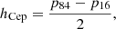
4.2.1. Total gas
In Fig. 2 we show the relations between Σgas and ΣSFR (left panel) and ρgas and ρSFR (right panel), with the points colour-coded according to the distance from the Galactic centre. We also include the sample of disc galaxies from B19 (grey points) in order to show that the MW follows the same trend as external galaxies. We note that the scatter is large in the surface-based panel, in particular for Σgas < 10 M⊙ pc−2. As shown in B19 (see left panel of Fig. 5b), a correlation close to  is visible at high densities, but some galaxies, including the MW, seem to follow a steeper relation with respect to the others.
 |
Fig. 2. Correlations between the surface density (left) and the volume density (right) of the gas and the SFR in the MW, colour-coded according to the Galactocentric radius. The squares indicate measurements for R ≤ R⊙ from Marasco et al. (2017), while the circles are for R > R⊙ from Binney & Merrifield (1998), Nakanishi & Sofue (2003, 2006), and Levine et al. (2006) (see text). The grey points are the corresponding quantites for the sample of 12 nearby disc galaxies (see Figs. 5 and 6 in B19 for the whole range of densities). The solid line in the right panel is the VSF law from B19 with its intrinsic scatter (red band). |
On the other hand, a different picture emerges from the right panel, where we can see that the MW volume densities follow remarkably well the VSF law with slope α = 1.91 (black solid line) and intrinsic scatter σ = 0.12 dex (red band) found in B19 for nearby galaxies. We recall that ρgas for the MW (Eq. (2)) was calculated using the scale heights derived with the hydrostatic equilibrium, consistently with the analysis done in B19 for nearby galaxies. Instead, ρSFR for the MW was estimated through Eq. (3) adopting the scale height of CCs, and not with Eq. (4) as was done for external galaxies. We discuss the relevance of this result in Sect. 5. For completeness, in Appendix C we compare the VSF law in Fig. 2 with the volume density of gas and SFR estimated using other measurements in the literature.
4.2.2. Atomic gas
In B19 we found that there is a surprisingly tight correlation with slope between 2.1 and 2.8 involving the atomic gas and the SFR volume densities. This is different with respect to the results obtained by other authors using the corresponding surface densities, that seems to be completely uncorrelated (e.g. Bigiel et al. 2010; Schruba et al. 2011).
The left panel of Fig. 3 shows the surface densities in the MW (points colour-coded using R) and in the sample of nearby disc galaxies of B19 (grey points). The MW is consistent with the other galaxies also in the plane ΣHI–ΣSFR, as in the case of total gas, and it is clear that there is very little or no correlation between these two quantities.
On the contrary, the right panel shows that the MW volume densities of atomic gas and SFR correlate, following remarkably well the VSF law with slope β = 2.79 ± 0.08 found for external galaxies. The validity of this relation in the MW confirms the link between atomic gas and star formation. We discuss this apparently controversial result in Sect. 5.2.
4.2.3. Molecular gas
The left panel of Fig. 4 shows the surface densities of molecular gas and SFR in the MW (coloured points) superimposed on those of the sample of disc galaxies in B19 (grey points). These latter were derived by Frank et al. (2016) using the CO conversion factor (αCO) measured by Sandstrom et al. (2013), which varies not only from galaxy to galaxy, but also with the galactocentric radius. The points of the MW are compatible with the relation obtained in B19 by fixing the slope to N = 1, as suggested by several authors (e.g. Wong & Blitz 2002; Kennicutt et al. 2007; Schruba et al. 2011; Marasco et al. 2012). We note that the molecular gas is not detected beyond R = 13 kpc, while ΣSFR is still measured.
Concerning the volume densities, the right panel of Fig. 4 shows that the MW points are compatible with external galaxies, given the large error bars mainly due to the uncertainty on αCO (see Bolatto et al. 2013). However, as we found in B19, the scatter of the relation is not significantly improved by the conversion from surface densities to volume densities. We also note that, by comparing Fig. 4 with Figs. 2 and 3, the scatter is larger in the case of molecular gas densities than in the case of atomic and total gas.
5. Discussion
5.1. Previous works on star formation laws in the Milky Way and nearby disc galaxies
Several studies in the literature aimed to find a model of star formation that could reproduce the radial profile of the SFR in our Galaxy, given a gas distribution.
For example, Boissier et al. (2003) adopted the Toomre criterion for the stability of galactic discs (Toomre 1964) proposed by Wang & Silk (1994), in order to account for the contribution of the stellar disc. They found that this criterion applies in the MW, but it has limited success in reproducing the profiles of the SFR surface densities in their sample of 16 disc galaxies. Moreover, the authors investigated the validity of the classical SK law,  (Kennicutt 1998), and of two modified versions that make use of the galactic orbital time,
 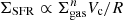 (Ohnishi 1975), and of the stellar surface density,
 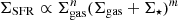 (Dopita & Ryder 1994)5. They found that the two modified versions of the SK law work slightly better than the classical relation in both the MW and the external galaxies, but the scatter remains large. It is interesting to note that both modified SK relations are in some way included in our VSF law. Indeed, the orbital time and, in particular, the rotation curve of a galaxy depend on its gravitational potential, hence including this term in the correlation could partially account for the role of the gravitational pull in shaping the gas vertical distribution (see Eq. (1)). Moreover, the stellar mass component dominates the gravitational potential in the inner regions of disc galaxies, hence the scale height significantly depends on the stellar distribution.
Our approach is based on the assumption that the vertical distribution of gas in galaxies is shaped by the hydrostatic equilibrium. This idea shares similarities with that proposed by Blitz & Rosolowsky (2006, hereafter BR06). These authors collected a sample of 14 nearby star-forming galaxies, including both dwarfs and spirals, and HI-rich and H2-rich galaxies. They found that the ratio of the molecular to the atomic gas content correlates with the midplane pressure calculated using the hydrostatic equilibrium. Therefore, they proposed that this hydrostatic pressure regulates the SFR surface density, which has two formulations, one when low-pressure (HI-dominated) environments are considered and the other for high-pressure (H2-dominated) environments. These results are somewhat different from ours as we do not find two regimes of star formation, but instead a monotonic relation that encompasses the HI- and H2-dominated regions. We think that these differences may be explained, at least partially, by drawbacks in the BR06 methodology. The most critical is that they neglected the dark matter component in the mass distribution calculation. As a consequence, their gravitational force and hydrostatic pressure are significantly underestimated, in particular in the outer regions of galaxies. Moreover, they ignored the radial gradient of the circular speed (e.g. Bahcall 1984; Bahcall & Casertano 1984; Olling 1995). This term is non-negligible in the inner regions of galaxies, where most star formation takes place, and has an impact on the correct determination of the hydrostatic pressure. Finally, BR06 assumed that the gas velocity dispersion is constant with the galactocentric radius at 8 km s−1, which is a factor of 1.5–2 lower than the typical values in the inner regions of galaxies (e.g. Fraternali et al. 2002; Boomsma et al. 2008, and B19).
Recently, Sofue (2017, hereafter S17) used the volume densities and the surface densities to study power-law correlations between the SFR and the atomic gas, the molecular gas, and the total gas in our Galaxy. He found that the index and the normalisation of all the power-laws both vary with the Galactocentric radius, and that all the relations tend to steepen in the outer regions of the Galaxy (8 kpc < R ≤ 20 kpc) with respect to the inner regions (0 kpc ≤ R ≤ 8 kpc), suggesting the existence of a density threshold6. In agreement with our findings, he obtained that the HI–SFR volume density correlations are steeper than those involving the total gas relations, which are in turn steeper than the H2–SFR relations. Despite evident similarities, there are significant differences between our approach and that of S17, as we discuss in Sect. 3.1 and Appendix A concerning the gas distribution. In addition, the SFR distribution adopted by S17 was derived in a previous paper (Sofue & Nakanishi 2017) using HII regions and adopting the kinematic distance method to infer their positions in the Galaxy. They decided to convert the surface density of SFR to the volume density using a constant value for hSFR as they found that the scale height of HII regions is ∼50 pc within R ≤ 10 kpc, showing clear flaring only beyond 15 kpc. This result is in contrast with that of Paladini et al. (2004), who also studied the distribution of HII regions, and with the measurements of the scale height of other SFR tracers (see Appendix B.2). Possibly, the hSFR by Sofue & Nakanishi (2017) is contaminated by the uncertainties on the distance determination related to the kinematic method, which we avoided by using standard candels as CCs. Interestingly, S17 also measured the index of the power laws considering the whole radial range, from 0 kpc to 20 kpc, and found 2.01 ± 0.02 for the correlation with the total gas volume density, 0.7 ± 0.07 for that with the molecular gas only, and 2.29 ± 0.3 for the atomic gas only, which are roughly consistent with our findings.
5.2. Physical interpretation of the VSF law with total gas
In our VSF law, the SFR volume density is regulated by the square of the total gas volume density. In the following, we discuss possible interpretations of this correlation. The first issue to bear in mind is that the correlations that we found are valid on kiloparsec scales, but are likely not applicable to a single molecular cloud or filament. Moreover, the exact value of α remains uncertain.
Our VSF law can be written as
 (5)
(5)
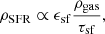
where ϵsf is a dimensionless efficiency parameter, usually assumed constant, and τsf is some physically meaningful timescale, which is different for different models and can have an explicit dependence on gas density. A natural timescale for star formation may be the free-fall time  (e.g. Madore 1977; Krumholz et al. 2012), which implies an index of 1.5. This is usually invoked to explain the SK relation with slope 1.4, with the implicit assumption of a constant scale height, both for the gas and the SFR distributions. In this work and in B19, we show that these scale heights instead increase with radius, for the MW and for nearby disc galaxies (see also Abramova & Zasov 2008 and Elmegreen 2015, 2018). Moreover, our results indicate that the slope is closer to ∼2 rather than 1.5, suggesting that another timescale is driving star formation on kiloparsec scales or is involved in the process. Potentially interesting and physically relevant timescales are the cooling time of warm gas (T ≈ 104 K) and the timescale to reach the equilibrium between the formation and destruction of H2, as suggested by Sofue (2017) for example. We note that both these timescales are inversely proportional to ρgas (see e.g. Hollenbach & McKee 1979; Ciotti & Ostriker 2007; Krumholz 2014), which, when inserted in Eq. (5), would predict a VSF with index 2, in agreement with our findings.
Leaving aside these considerations about the slope of the VSF law, it is interesting to qualitatively interpret our results in the picture of a self-regulating star formation model. Our ρgas is the highest gas density (i.e. that at the midplane) at which the pressure–gravity balance holds (see Eqs. (1) and (2)). Therefore, it is probably a good estimate of the gas volume density (averaged on kiloparsec scale) in star-forming clouds, as suggested by the small scatter of the VSF law. Turbulent motions are likely sustained by stellar feedback, whose strength is expected to be proportional to the SFR density itself. The higher the SFR density per unit volume, the more turbulent pressure helps thermal pressure to contrast gravity. As a consequence, the gas z-distribution broadens and the scale height increases, thus the volume density in the midplane decrease and so does the SFR density. Then the pressure support against gravity weakens because of the reduction of turbulence injection, and the gas z-distribution narrows, which increases the gas volume densities in the midplane and consequently the SFR density. However, the influence of stellar feedback on the ISM turbulence is still a matter of debate (e.g. Tamburro et al. 2009; Utomo et al. 2019) and we leave a detailed analysis of this to future investigations.
The above interpretation is similar to the self-regulating scenario proposed by Ostriker & Shetty (2011), who assumed that star formation in spiral galaxies is regulated by the pressure support of gas turbulence against gravity (the radiation pressure may become dominant in the most extreme starburst regions). Investigating the compatibility of this model with our results also goes beyond the scope of this paper.
The unexpected correlation between the SFR and the atomic gas volume densities suggests that the HI can be a good tracer of the star-forming gas over a broad range of densities, from dwarf to spiral galaxies. On the contrary, the scatter in the H2–SFR relations is large, with no improvement from the conversion of surface densities to volume densities. In addition, the molecular gas, which is usually traced using CO emission, is often detected only in the inner regions of star-forming galaxies (including the MW). This may seem counter-intuitive, as star formation is observed to occur in molecular clouds. A possible explanation of the HI–SFR correlation is that molecular clouds form from the atomic gas and are rapidly swept away by stellar feedback, leaving only the parent atomic gas. Therefore, we could expect to see the HI–SFR correlation if the timescale for the formation of a new molecular clouds were longer than the lifetime of star formation tracers7. In low-density and/or metal-poor regions, the CO emission likely becomes a bad tracer of the total molecular gas (H2) (e.g. Schruba et al. 2012; Hunt et al. 2015; Seifried et al. 2017). The existence of a HI-VSF law that extends to these environments seems to indicate that HI can efficiently trace also the CO-dark H2. Nevertheless, this correlation may also suggest that the atomic gas has an important, albeit non-trivial, role in star formation, and that the molecular gas is not always a prerequisite for creating new stars (Glover & Clark 2012; Krumholz 2012).
6. Summary and conclusions
Star formation laws are undoubtedly of fundamental importance to understand galaxy formation and evolution. It is generally acknowledged that the formation of stars in galaxies is regulated by their gas reservoir, but studying the intrinsic distributions of the gas and the SFR is hampered by the difficulty of measuring the volume densities in galaxies. The surface densities, observable in external galaxies, are affected by projection effects due to the flaring of the thickness of gas discs. Therefore, the relation between the surface density and the volumetric density is non-trivial and similar values of surface density can be measured where the volume density is low and the gas disc is thick, or vice versa.
In B19, we used a sample of 12 nearby disc galaxies to derive the volume densities of the gas (HI and H2) from the observed surface densities using the scale height calculated under the assumption of hydrostatic equilibrium in the galactic gravitational potential. We find that the gas and the SFR volume densities correlate following a tight power-law relation, the VSF law, whose index is either ∼1.3 or ∼1.9 depending on whether the scale height of the SFR distribution is assumed to be constant or flaring with the galactocentric radius.
In this work we investigated the VSF law in our Galaxy using the same method as for external galaxies, but with a crucial improvement. We used CCs as tracers of the recent star formation and thereby directly derived the thickness of their vertical distribution as a function of the Galactocentric radius. This allowed us to convert the SFR surface density to volume density, and to find a unique slope of the VSF law. Our main conclusions are the following:
-
The vertical distribution of the SFR density flares with the Galactocentric radius and its scale height is fully compatible with the scale height of cold gas (HI+H2) calculated assuming the hydrostatic equilibrium.
-
We explored the correlations between the volume density of the SFR and the volume densities of the total gas, the atomic gas only, and the molecular gas only, finding that the MW follows the same relations found in nearby disc galaxies.
-
The VSF law with total gas
 is the tightest correlation and α ≈ 2.
We note that the flaring of gas thickness is significant and must be taken into account in the studies of gas distribution in galaxies, not only in dwarfs but also in spirals (see Wilson et al. 2019 for an application to ultra-luminous infrared galaxies). The VSF law is described by a single index across the whole density range, which means that there is no volume density threshold and that the breaks previously observed in the resolved and integrated SK laws are due to the disc flaring, rather than to a drop in the star formation efficiency (see also Elmegreen 2015, 2018).
A physical interpretation of the VSF law is currently lacking and we hope that it will stimulate future investigations. The assumption of the hydrostatic equilibrium for the gas in galaxies should also be tested, but measuring the vertical distribution of gas in galaxies is not an easy task.
Our VSF laws are simple recipes for star formation that could be included in analytical or semi-analytical models of the formation and evolution of galaxies. Moreover, the VSF laws could be easily compared with the correlations between the SFR and the gas volume densities predicted by numerical simulations of star formation on small scales, with the advantage of avoiding the 2D projection to obtain the surface densities involved in the SK law.
The extra-planar gas is a faint layer of HI, observed both in the MW and in nearby galaxies (Fraternali et al. 2001; Oosterloo et al. 2007; Gentile et al. 2013; Marasco et al. 2019), which is likely generated by the galactic fountain flow (Fraternali 2017). This component rotates with slower velocity with respect to the midplane gas, and reaches heights of a few kpc above the disc. If not taken into account, the extra-planar gas can lead to a slight overestimation of the scale height (∼20% for our Galaxy; see Marasco et al. 2017).
We did not include the Kalberla & Dedes (2008) measurements in the estimate of our fiducial ΣHI as their density profile is more than a factor of 2 higher than the other estimates in the literature (see Appendix A.1).
In the MW, SNRs can be considered good tracers of recent (≲50 Myr) star formation events as, in Sbc galaxies, the rate of SNe Ia is ∼4 − 5 times lower than the rate of SNe II and Ibc (Li et al. 2011).
This formulation is almost equivalent to the so-called extended-Schmidt law (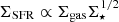 ), which was originally proposed by Talbot & Arnett (1975) and then observationally studied by Shi et al. (2011, 2018) and Roychowdhury et al. (2017).
The variation of the index and the normalisation was also measured on shorter scales by dividing the Galaxy in annulii of 2 kpc width.
The timescale of molecular cloud formation depends on the physical mechanism that regulates the process. It is probably between a few 107 yr and 108 yr, subject to the ISM local conditions (see e.g. McKee & Ostriker 2007). Star formation tracers are characterised by timescales that typically range from a few 106 yr to about 108 yr (Kennicutt & Evans 2012). Therefore, the comparison between the two timescales is very uncertain.
Nakanishi & Sofue (2003) assumed a sech2 profile for the HI vertical distribution, so we rescaled their HWHM by a factor 0.8 to obtain the equivalent quantity for a Gaussian profile.
Acknowledgments
We are grateful to the anonymous referee for the useful comments that helped to improve the paper. We would like to thank X. Chen, T. Mackereth, and Y. Sofue for sharing their data and results. FF and AM thank Lotte Elzinga for her preliminary investigation of hydrostatic equilibrium in the Milky Way during her Bachelor project. GP acknowledges support by the Swiss National Science Foundation, grant PP00P2_163824. GI is supported by the Royal Society Newton International Fellowship (NF170902).
References
- Abramova, O. V., & Zasov, A. V. 2008, Astron. Rep., 52, 257 [NASA ADS] [CrossRef] [Google Scholar]
- Armillotta, L., Krumholz, M. R., Di Teodoro, E. M., & McClure-Griffiths, N. M. 2019, MNRAS, 490, 4401 [NASA ADS] [CrossRef] [Google Scholar]
- Bacchini, C., Fraternali, F., Iorio, G., & Pezzulli, G. 2019, A&A, 622, A64 [NASA ADS] [CrossRef] [EDP Sciences] [Google Scholar]
- Bahcall, J. N. 1984, ApJ, 276, 156 [NASA ADS] [CrossRef] [Google Scholar]
- Bahcall, J. N., & Casertano, S. 1984, ApJ, 284, L35 [NASA ADS] [CrossRef] [Google Scholar]
- Bigiel, F., Leroy, A., Walter, F., et al. 2008, AJ, 136, 2846 [NASA ADS] [CrossRef] [Google Scholar]
- Bigiel, F., Leroy, A., Walter, F., et al. 2010, AJ, 140, 1194 [NASA ADS] [CrossRef] [Google Scholar]
- Binney, J., & Merrifield, M. 1998, Galactic Astronomy (Princeton: Princeton University Press) [Google Scholar]
- Binney, J., Gerhard, O. E., Stark, A. A., Bally, J., & Uchida, K. I. 1991, MNRAS, 252, 210 [NASA ADS] [CrossRef] [Google Scholar]
- Blitz, L., & Rosolowsky, E. 2006, ApJ, 650, 933 [NASA ADS] [CrossRef] [Google Scholar]
- Boissier, S., Prantzos, N., Boselli, A., & Gavazzi, G. 2003, MNRAS, 346, 1215 [NASA ADS] [CrossRef] [Google Scholar]
- Bolatto, A. D., Leroy, A. K., Jameson, K., et al. 2011, ApJ, 741, 12 [NASA ADS] [CrossRef] [Google Scholar]
- Bolatto, A. D., Wolfire, M., & Leroy, A. K. 2013, ARA&A, 51, 207 [Google Scholar]
- Bono, G., Marconi, M., Cassisi, S., et al. 2005, ApJ, 621, 966 [NASA ADS] [CrossRef] [Google Scholar]
- Boomsma, R., Oosterloo, T. A., Fraternali, F., van der Hulst, J. M., & Sancisi, R. 2008, A&A, 490, 555 [NASA ADS] [CrossRef] [EDP Sciences] [Google Scholar]
- Bronfman, L., Cohen, R. S., Alvarez, H., May, J., & Thaddeus, P. 1988, ApJ, 324, 248 [NASA ADS] [CrossRef] [Google Scholar]
- Bronfman, L., Casassus, S., May, J., & Nyman, L.-Å. 2000, A&A, 358, 521 [NASA ADS] [Google Scholar]
- Burton, W. B., & Gordon, M. A. 1978, A&A, 63, 7 [NASA ADS] [Google Scholar]
- Burton, W. B. 1974, in Galactic Radio Astronomy, eds. F. J. Kerr, & S. C. Simonson, IAU Symp., 60, 551 [NASA ADS] [CrossRef] [Google Scholar]
- Caputo, F., Marconi, M., & Musella, I. 2000, A&A, 354, 610 [NASA ADS] [Google Scholar]
- Case, G. L., & Bhattacharya, D. 1998, ApJ, 504, 761 [Google Scholar]
- Chen, X., Wang, S., Deng, L., et al. 2019, Nat. Astron., 3, 320 [NASA ADS] [CrossRef] [Google Scholar]
- Chomiuk, L., & Povich, M. S. 2011, AJ, 142, 197 [NASA ADS] [CrossRef] [Google Scholar]
- Ciotti, L., & Ostriker, J. P. 2007, ApJ, 665, 1038 [NASA ADS] [CrossRef] [Google Scholar]
- Clemens, D. P., Sanders, D. B., & Scoville, N. Z. 1988, ApJ, 327, 139 [NASA ADS] [CrossRef] [Google Scholar]
- Dame, T. M., Ungerechts, H., Cohen, R. S., et al. 1987, ApJ, 322, 706 [NASA ADS] [CrossRef] [Google Scholar]
- Dame, T. M., Hartmann, D., & Thaddeus, P. 2001, ApJ, 547, 792 [NASA ADS] [CrossRef] [Google Scholar]
- de los Reyes, M. A. C., & Kennicutt, Jr., R. C. 2019, ApJ, 872, 16 [NASA ADS] [CrossRef] [Google Scholar]
- Dehnen, W., & Binney, J. 1998, MNRAS, 294, 429 [NASA ADS] [CrossRef] [Google Scholar]
- Dékány, I., Hajdu, G., Grebel, E. K., & Catelan, M. 2019, ApJ, 883, 58 [NASA ADS] [CrossRef] [Google Scholar]
- Dessauges-Zavadsky, M., Verdugo, C., Combes, F., & Pfenniger, D. 2014, A&A, 566, A147 [NASA ADS] [CrossRef] [EDP Sciences] [Google Scholar]
- Dickey, J. M., & Lockman, F. J. 1990, ARA&A, 28, 215 [NASA ADS] [CrossRef] [MathSciNet] [Google Scholar]
- Digel, S. W. 1991, PhD Thesis, Harvard University, Cambridge, MA [Google Scholar]
- Dopita, M. A., & Ryder, S. D. 1994, ApJ, 430, 163 [NASA ADS] [CrossRef] [Google Scholar]
- Elmegreen, B. G. 2015, ApJ, 814, L30 [NASA ADS] [CrossRef] [Google Scholar]
- Elmegreen, B. G. 2018, ApJ, 854, 16 [NASA ADS] [CrossRef] [Google Scholar]
- Frank, B. S., de Blok, W. J. G., Walter, F., Leroy, A., & Carignan, C. 2016, AJ, 151, 94 [NASA ADS] [CrossRef] [Google Scholar]
- Fraternali, F. 2017, in Gas Accretion onto Galaxies, eds. A. Fox, & R. Davé, Astrophys. Space Sci. Lib., 430, 323 [NASA ADS] [CrossRef] [Google Scholar]
- Fraternali, F., & Tomassetti, M. 2012, MNRAS, 426, 2166 [NASA ADS] [CrossRef] [Google Scholar]
- Fraternali, F., Oosterloo, T., Sancisi, R., & van Moorsel, G. 2001, ApJ, 562, L47 [NASA ADS] [CrossRef] [Google Scholar]
- Fraternali, F., van Moorsel, G., Sancisi, R., & Oosterloo, T. 2002, AJ, 123, 3124 [NASA ADS] [CrossRef] [Google Scholar]
- Freedman, D., & Diaconis, P. 1981, Zeitschrift für Wahrscheinlichkeitstheorie und Verwandte Gebiete, 57, 453 [Google Scholar]
- Gentile, G., Józsa, G. I. G., Serra, P., et al. 2013, A&A, 554, A125 [NASA ADS] [CrossRef] [EDP Sciences] [Google Scholar]
- Glover, S. C. O., & Clark, P. C. 2012, MNRAS, 421, 9 [NASA ADS] [Google Scholar]
- Grabelsky, D. A., Cohen, R. S., Bronfman, L., Thaddeus, P., & May, J. 1987, ApJ, 315, 122 [NASA ADS] [CrossRef] [Google Scholar]
- Green, D. A. 2015, MNRAS, 454, 1517 [NASA ADS] [CrossRef] [Google Scholar]
- Heyer, M. H., Corbelli, E., Schneider, S. E., & Young, J. S. 2004, ApJ, 602, 723 [NASA ADS] [CrossRef] [Google Scholar]
- Hollenbach, D., & McKee, C. F. 1979, ApJS, 41, 555 [NASA ADS] [CrossRef] [Google Scholar]
- Hunt, L. K., García-Burillo, S., Casasola, V., et al. 2015, A&A, 583, A114 [NASA ADS] [CrossRef] [EDP Sciences] [Google Scholar]
- Iorio, G. 2018, PhD Thesis, University of Bologna [Google Scholar]
- Jones, E., Oliphant, T., Peterson, P., et al. 2001, SciPy: Open Source Scientific tools for Python [Google Scholar]
- Kalberla, P. M. W., & Dedes, L. 2008, A&A, 487, 951 [NASA ADS] [CrossRef] [EDP Sciences] [Google Scholar]
- Kalberla, P. M. W., & Kerp, J. 1998, A&A, 339, 745 [NASA ADS] [Google Scholar]
- Kalberla, P. M. W., Burton, W. B., Hartmann, D., et al. 2005, A&A, 440, 775 [NASA ADS] [CrossRef] [EDP Sciences] [Google Scholar]
- Kalberla, P. M. W., Dedes, L., Kerp, J., & Haud, U. 2007, A&A, 469, 511 [NASA ADS] [CrossRef] [EDP Sciences] [Google Scholar]
- Kennicutt, Jr., R. C. 1989, ApJ, 344, 685 [NASA ADS] [CrossRef] [Google Scholar]
- Kennicutt, Jr., R. C. 1998, ApJ, 498, 541 [NASA ADS] [CrossRef] [Google Scholar]
- Kennicutt, R. C., & Evans, N. J. 2012, ARA&A, 50, 531 [NASA ADS] [CrossRef] [Google Scholar]
- Kennicutt, Jr., R. C., Calzetti, D., Walter, F., et al. 2007, ApJ, 671, 333 [NASA ADS] [CrossRef] [Google Scholar]
- Koyama, H., & Ostriker, E. C. 2009, ApJ, 693, 1346 [NASA ADS] [CrossRef] [Google Scholar]
- Kramer, E. D., & Randall, L. 2016, ApJ, 829, 126 [NASA ADS] [CrossRef] [Google Scholar]
- Kroupa, P., & Weidner, C. 2003, ApJ, 598, 1076 [NASA ADS] [CrossRef] [Google Scholar]
- Krumholz, M. R. 2012, ApJ, 759, 9 [NASA ADS] [CrossRef] [Google Scholar]
- Krumholz, M. R. 2014, Phys. Rep., 539, 49 [NASA ADS] [CrossRef] [Google Scholar]
- Krumholz, M. R., Dekel, A., & McKee, C. F. 2012, ApJ, 745, 69 [NASA ADS] [CrossRef] [Google Scholar]
- Lada, C. J., Lombardi, M., & Alves, J. F. 2010, ApJ, 724, 687 [NASA ADS] [CrossRef] [Google Scholar]
- Lada, C. J., Lombardi, M., Roman-Zuniga, C., Forbrich, J., & Alves, J. F. 2013, ApJ, 778, 133 [NASA ADS] [CrossRef] [Google Scholar]
- Leavitt, H. S., & Pickering, E. C. 1912, Harv. Coll. Obs. Circ., 173, 1 [Google Scholar]
- Leroy, A. K., Walter, F., Brinks, E., et al. 2008, AJ, 136, 2782 [NASA ADS] [CrossRef] [Google Scholar]
- Levine, E. S., Blitz, L., & Heiles, C. 2006, ApJ, 643, 881 [NASA ADS] [CrossRef] [Google Scholar]
- Li, C., Zhao, G., Jia, Y., et al. 2019, ApJ, 871, 208 [NASA ADS] [CrossRef] [Google Scholar]
- Li, W., Chornock, R., Leaman, J., et al. 2011, MNRAS, 412, 1473 [NASA ADS] [CrossRef] [Google Scholar]
- Liszt, H. S. 1992, in The Center, Bulge, and Disk of the Milky Way, ed. L. Blitz, Astrophys. Space Sci. Lib., 180, 111 [NASA ADS] [CrossRef] [Google Scholar]
- Liu, G., Koda, J., Calzetti, D., Fukuhara, M., & Momose, R. 2011, ApJ, 735, 63 [NASA ADS] [CrossRef] [Google Scholar]
- Lockman, F. J. 1984, ApJ, 283, 90 [NASA ADS] [CrossRef] [Google Scholar]
- Luna, A., Bronfman, L., Carrasco, L., & May, J. 2006, ApJ, 641, 938 [NASA ADS] [CrossRef] [Google Scholar]
- Lyne, A. G., Manchester, R. N., & Taylor, J. H. 1985, MNRAS, 213, 613 [NASA ADS] [CrossRef] [Google Scholar]
- Mackereth, J. T., Bovy, J., Schiavon, R. P., et al. 2017, MNRAS, 471, 3057 [NASA ADS] [CrossRef] [Google Scholar]
- Madore, B. F. 1977, MNRAS, 178, 1 [NASA ADS] [CrossRef] [Google Scholar]
- Marasco, A., & Fraternali, F. 2011, A&A, 525, A134 [NASA ADS] [CrossRef] [EDP Sciences] [Google Scholar]
- Marasco, A., Fraternali, F., & Binney, J. J. 2012, MNRAS, 419, 1107 [NASA ADS] [CrossRef] [Google Scholar]
- Marasco, A., Fraternali, F., van der Hulst, J. M., & Oosterloo, T. 2017, A&A, 607, A106 [NASA ADS] [CrossRef] [EDP Sciences] [Google Scholar]
- Marasco, A., Fraternali, F., Heald, G., et al. 2019, A&A, 631, A50 [NASA ADS] [CrossRef] [EDP Sciences] [Google Scholar]
- Martin, C. L., & Kennicutt, Jr., R. C. 2001, ApJ, 555, 301 [NASA ADS] [CrossRef] [Google Scholar]
- McKee, C. F., & Ostriker, E. C. 2007, ARA&A, 45, 565 [NASA ADS] [CrossRef] [Google Scholar]
- McMillan, P. J. 2011, MNRAS, 414, 2446 [NASA ADS] [CrossRef] [Google Scholar]
- McMillan, P. J. 2017, MNRAS, 465, 76 [NASA ADS] [CrossRef] [Google Scholar]
- Misiriotis, A., Xilouris, E. M., Papamastorakis, J., Boumis, P., & Goudis, C. D. 2006, A&A, 459, 113 [NASA ADS] [CrossRef] [EDP Sciences] [Google Scholar]
- Muñoz-Mateos, J. C., Boissier, S., de Paz, A. G., et al. 2011, ApJ, 731, 10 [NASA ADS] [CrossRef] [Google Scholar]
- Nakanishi, H., & Sofue, Y. 2003, PASJ, 55, 191 [Google Scholar]
- Nakanishi, H., & Sofue, Y. 2006, PASJ, 58, 847 [NASA ADS] [Google Scholar]
- Ohnishi, T. 1975, Progr. Theor. Phys., 53, 1042 [NASA ADS] [CrossRef] [Google Scholar]
- Olling, R. P. 1995, AJ, 110, 591 [NASA ADS] [CrossRef] [Google Scholar]
- Oosterloo, T., Fraternali, F., & Sancisi, R. 2007, AJ, 134, 1019 [NASA ADS] [CrossRef] [Google Scholar]
- Ostriker, E. C., & Shetty, R. 2011, ApJ, 731, 41 [NASA ADS] [CrossRef] [Google Scholar]
- Paladini, R., Davies, R. D., & De Zotti, G. 2004, MNRAS, 347, 237 [NASA ADS] [CrossRef] [Google Scholar]
- Pezzulli, G., Fraternali, F., Boissier, S., & Muñoz-Mateos, J. C. 2015, MNRAS, 451, 2324 [NASA ADS] [CrossRef] [Google Scholar]
- Pfrommer, C., Pakmor, R., Schaal, K., Simpson, C. M., & Springel, V. 2017, MNRAS, 465, 4500 [NASA ADS] [CrossRef] [Google Scholar]
- Ripepi, V., Molinaro, R., Musella, I., et al. 2019, A&A, 625, A14 [NASA ADS] [CrossRef] [EDP Sciences] [Google Scholar]
- Roychowdhury, S., Chengalur, J. N., & Shi, Y. 2017, A&A, 608, A24 [NASA ADS] [CrossRef] [EDP Sciences] [Google Scholar]
- Sanders, D. B., Solomon, P. M., & Scoville, N. Z. 1984, ApJ, 276, 182 [NASA ADS] [CrossRef] [Google Scholar]
- Sandstrom, K. M., Leroy, A. K., Walter, F., et al. 2013, ApJ, 777, 5 [NASA ADS] [CrossRef] [Google Scholar]
- Schaye, J. 2004, ApJ, 609, 667 [NASA ADS] [CrossRef] [Google Scholar]
- Schmidt, M. 1959, ApJ, 129, 243 [NASA ADS] [CrossRef] [Google Scholar]
- Schruba, A., Leroy, A. K., Walter, F., et al. 2011, AJ, 142, 37 [NASA ADS] [CrossRef] [Google Scholar]
- Schruba, A., Leroy, A. K., Walter, F., et al. 2012, AJ, 143, 138 [NASA ADS] [CrossRef] [Google Scholar]
- Seifried, D., Walch, S., Girichidis, P., et al. 2017, MNRAS, 472, 4797 [NASA ADS] [CrossRef] [Google Scholar]
- Sellwood, J. A. 2014, Rev. Mod. Phys., 86, 1 [NASA ADS] [CrossRef] [Google Scholar]
- Shi, Y., Helou, G., Yan, L., et al. 2011, ApJ, 733, 87 [NASA ADS] [CrossRef] [Google Scholar]
- Shi, Y., Yan, L., Armus, L., et al. 2018, ApJ, 853, 149 [NASA ADS] [CrossRef] [Google Scholar]
- Simpson, C. M., Pakmor, R., Marinacci, F., et al. 2016, ApJ, 827, L29 [NASA ADS] [CrossRef] [Google Scholar]
- Skowron, D. M., Skowron, J., Mróz, P., et al. 2019, Science, 365, 478 [NASA ADS] [CrossRef] [Google Scholar]
- Sofue, Y. 2017, MNRAS, 469, 1647 [NASA ADS] [CrossRef] [Google Scholar]
- Sofue, Y., & Nakanishi, H. 2017, PASJ, 69, 19 [NASA ADS] [CrossRef] [Google Scholar]
- Sormani, M. C., Binney, J., & Magorrian, J. 2015, MNRAS, 454, 1818 [NASA ADS] [CrossRef] [Google Scholar]
- Sormani, M. C., & Magorrian, J. 2015, MNRAS, 446, 4186 [NASA ADS] [CrossRef] [Google Scholar]
- Talbot, Jr., R. J., & Arnett, W. D. 1975, ApJ, 197, 551 [NASA ADS] [CrossRef] [Google Scholar]
- Tamburro, D., Rix, H.-W., Leroy, A. K., et al. 2009, AJ, 137, 4424 [NASA ADS] [CrossRef] [Google Scholar]
- Toomre, A. 1964, ApJ, 139, 1217 [Google Scholar]
- Utomo, D., Blitz, L., & Falgarone, E. 2019, ApJ, 871, 17 [NASA ADS] [CrossRef] [Google Scholar]
- Wang, B., & Silk, J. 1994, ApJ, 427, 759 [NASA ADS] [CrossRef] [Google Scholar]
- Wang, H.-F., Liu, C., Xu, Y., Wan, J.-C., & Deng, L. 2018, MNRAS, 478, 3367 [NASA ADS] [CrossRef] [Google Scholar]
- Westerhout, G. 1957, Bull. Astron. Inst. Neth., 13, 201 [NASA ADS] [Google Scholar]
- Wilson, C. D., Elmegreen, B. G., Bemis, A., & Brunetti, N. 2019, ApJ, 882, 5 [NASA ADS] [CrossRef] [Google Scholar]
- Wong, T., & Blitz, L. 2002, ApJ, 569, 157 [NASA ADS] [CrossRef] [Google Scholar]
- Wouterloot, J. G. A., Brand, J., Burton, W. B., & Kwee, K. K. 1990, A&A, 230, 21 [NASA ADS] [Google Scholar]
- Yusifov, I., & Küçük, I. 2004, A&A, 422, 545 [NASA ADS] [CrossRef] [EDP Sciences] [Google Scholar]
Appendix A: The Milky Way gas distribution compared with the literature
In the following, we compare the radial profiles of the surface density, the volume density, and the scale height adopted in this work with those available in the literature, for the HI, the H2, and the total gas.
A.1. Gas surface densities
Figure A.1 shows the radial profiles of the surface density of the atomic gas (left), the molecular gas (centre), and the total gas (right) in the MW (all profiles rescaled to the same value for R⊙). The black points represent the profiles adopted in this work, which were calculated using profiles from the literature smoothed to 1 kpc resolution. For example, at 8 kpc we used the measurements of the surface density from 7.5 kpc to 8.5 kpc and fitted a Gaussian distribution to the data (accounting for the errors). The resulting best-fit Gaussian is centred on the final value for the density (i.e. the black point at 8 kpc) and its standard deviation is a first estimate of the error. We adopted the same procedure for the HI and H2 profiles. These fiducial profiles are compared to those in the literature, whose reference papers are indicated by the initials in the legend of Fig. A.1.
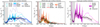 |
Fig. A.1. Surface density radial profiles of the atomic gas (left), the molecular gas (centre), and the total gas (right) from the literature compared to the profile adopted in this work (black points). The factor 1.36 for the helium correction is included. Left panel: BG78 = Burton & Gordon (1978), Wo90 = Wouterloot et al. (1990), DL90 = Dickey & Lockman (1990), BM98 = Binney & Merrifield (1998), NS03 = Nakanishi & Sofue (2003), Le06 = Levine et al. (2006), KD08 = Kalberla & Dedes (2008), and M17 = Marasco et al. (2017). Centre panel: Sa84 = Sanders et al. (1984), Da87 = Dame et al. (1987), Gr87 = Grabelsky et al. (1987), Br88 = Bronfman et al. (1988), Cl88 = Clemens et al. (1988), Di91 = Digel (1991), Lu00 = Luna et al. (2006), NS06 = Nakanishi & Sofue (2006). |
Within the solar circle, we used ΣHI and ΣH2 from Marasco et al. (2017). The upper errors on ΣHI were estimated from the standard deviation of the Gaussian, while the lower errors were found using ΣHI derived in optically thin regime (see Marasco et al. 2017 for details). This sort of correction was done for consistency with B19, in which we used ΣHI of external galaxies derived under the assumption of 100% optically thin HI. Concerning the molecular gas, we followed the Marasco et al. (2017) approach and associated an error of 30% to ΣH2 based on the uncertainty on the CO–H2 conversion factor estimated by Bolatto et al. (2013).
Beyond the solar circle, we adopted ΣHI profiles from Binney & Merrifield (1998), Nakanishi & Sofue (2003), and Levine et al. (2006). These authors assumed an opaque regime for the HI, but did not explore the optically thin case, thus we used the Gaussian standard deviation for the error. Similarly, ΣH2(R) was derived using the estimates by Nakanishi & Sofue (2006) and Binney & Merrifield (1998), and we associated a 30% uncertainty based on Bolatto et al. (2013).
The most uncertain profile is probably ΣHI (see Fig. A.1), while the different estimates of ΣH2 seem approximately compatible. The discrepancies between the HI profiles could be due to the differences in the assumed rotation curve, which has an important effect on the kinematic distance method (see Burton 1974; Marasco et al. 2017).
A.2. Gas scale height
There have been several attempts to infer the gas scale height in our Galaxy directly from the data, and it is interesting to compare these determinations with those we calculated with the hydrostatic equilibrium (see Sect. 4.1). These latter are represented by the black points in Fig. A.2, where the left and the right panel respectively show the HI and the H2 scale heights.
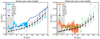 |
Fig. A.2. Scale height radial profiles of the atomic and molecular gas from the literature (Lo84 = Lockman 1984; see caption of Fig. A.1 for the other labels in the legend) compared to those calculated assuming the hydrostatic equilibrium (black points). |
Despite the very different methods, all the profiles show a flaring. The scale height of HI in hydrostatic equilibrium is compatible with the results of Lockman (1984), Wouterloot et al. (1990), Levine et al. (2006), and Kalberla & Dedes (2008). The last work in particular assumed the hydrostatic equilibrium a priori and modelled the ISM as a two-phase fluid, in which the warm neutral medium (WNM) and the cold neutral medium (CNM) have different scale heights. They found that the final model is close to a single-component medium with constant velocity dispersion at 8.3 km s−1, which is similar to the values we adopted for the HI. This can explain the agreement between the scale heights, despite the significant differences between the mass models (see Kalberla et al. 2007).
However, our scale height differs from those derived by Nakanishi & Sofue (2003)8 and Marasco et al. (2017) by ∼50% (see left panel in Fig. A.2). Nakanishi & Sofue (2003) adopted the kinematic distance method to measure the HI distribution and removed the emission of high-altitude and diffuse HI, so a direct comparison is not straightforward. The discrepancy with Marasco et al. (2017) scale height deserves further discussions, as we adopted their velocity dispersion profile to calculate hHI, hence we expected the scale heights to be compatible within the uncertainties. There are some possible explanations for this difference. Marasco et al. (2017) found that HI in the midplane could be best described by a two-component model, where 80–85% of the atomic gas has low velocity dispersion (∼8 km s−1), while the remaining has a much higher velocity dispersion (15–20 km s−1). Likely, this second component has a larger scale height than the first one, in which case it could dominate the HI emission above the midplane. The vertical distribution of the gas was instead modelled using a single component, thus it is possible that the resulting hHI is closer to the scale height of the high-σHI component than to that of the low-σHI one. We adopted the measured velocity dispersion to calculate the scale height with hydrostatic equilibrium, but this approach implicitly relies on the assumption that the velocity dispersion is isotropic and constant along z. However, this latter property may not be true if the high-σHI component is more abundant than the low-σHI one at high latitudes above the midplane. Alternatively, we could speculate that some anisotropic force contributes to balancing the gravitational pull towards the midplane, for instance magnetic tension or cosmic rays. In particular, recent magneto-hydrodynamical simulations of stratified gas of galaxies (e.g. Simpson et al. 2016; Pfrommer et al. 2017) show that the anisotropic diffusion of cosmic rays can contribute to the vertical gradient of the gas pressure, but investigating such scenarios is beyond the aim of this paper.
Figure A.2 shows that the molecular gas scale height based on the hydrostatic equilibrium resembles the hH2 profiles found by Nakanishi & Sofue (2006) and Marasco et al. (2017) within the uncertainties. The hH2 profiles from Sanders et al. (1984), Grabelsky et al. (1987), and Wouterloot et al. (1990) are also in approximate agreement with our scale height, while the Bronfman et al. (1988) scale height shows some discrepancies for 3 kpc ≲R ≲ 8 kpc.
A.3. Gas volume densities
In Fig. A.3, the black points represent the MW volume density profiles of atomic gas (left panel), molecular gas (central panel), and total gas (right panel) calculated with the scale height of hydrostatic equilibrium. The other points show instead the measurements available in the literature.
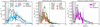 |
Fig. A.3. Volume density radial profiles of the atomic gas (left), the molecular gas (centre), and the total gas (right) from the literature (Li92 = Liszt 1992, KK98 = Kalberla & Kerp 1998, NS = HI from Nakanishi & Sofue 2003, and H2 from Nakanishi & Sofue 2006; see caption of Fig. A.1 for the other labels in the legend) compared to the profile adopted in this work (black points). The factor 1.36 for the helium correction is included. |
Within the solar radius, our ρHI is systematically higher than the other estimates, as we expected from the discrepancy found between the scale heights. However, this difference seems to be partially accounted for by the error bars, which were calculated from the uncertainties on hHI and ΣHI. These latter in particular include the difference between the profiles in the literature (beyond R⊙) and the uncertainty on the optical regime of atomic gas (within R⊙), as reported in Appendix A.1. Concerning the molecular gas, our profile for ρH2(R) is in agreement with the observations, and given that the gas is mainly molecular within the solar circle, our profile for the total gas is also approximately compatible with all the other determinations.
Appendix B: Milky Way SFR distribution using different tracers
In the following, we compare the surface density and the scale height of the SFR adopted in this work with other profiles available in the literature.
B.1. SFR surface density
We adopted the SFR surface density profile derived by Green (2015) using SNRs to trace the distribution of recent star formation. In the left panel of Fig. B.1, this profile is compared to others in the literature, all normalised to have a total SFR of 1.9 M⊙ yr−1. The discrepancy with Case & Bhattacharya (1998), who also studied the SNR distribution, was expected (see Green 2015). The adopted ΣSFR(R) is compatible with the profile derived using pulsars (Lyne et al. 1985; Yusifov & Küçük 2004) and the far-infrared emission (Misiriotis et al. 2006), except for the inner 3 kpc that are not included in our study. The Green (2015) profile is also compatible with the HII regions radial distribution (Paladini et al. 2004), except for R ∼ 5 − 6 kpc (see Appendix C for further discussion).
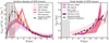 |
Fig. B.1. Surface density (left panel) and scale height (right panel) of the SFR distribution using different tracers. The black points show the profile adopted in this work, while the others are different estimates from the literature (see text). The reference papers are indicated by the following abbreviations: L85 = Lyne et al. (1985), CB98 = Case & Bhattacharya (1998), YK04 = Yusifov & Küçük (2004), G15 = Green (2015), B00 = Bronfman et al. (2000), and L19 = Li et al. (2019). |
B.2. SFR scale height
We studied the radial profile of CCs scale height using the residual z-coordinate (Δz) provided by Chen et al. (2019), see their Fig. 4), for which the signature of the Galactic warp was already modelled and filtred out. We built radial bins of ΔR = 1 kpc from R = 5 kpc to R = 19 kpc containing enough stars (from 8 to 200) to obtain a reasonable sampling of their vertical distribution in each bin using the Freedman–Diaconis estimator (Freedman & Diaconis 1981) implemented in the scipy Python package (Jones et al. 2001). By analogy with a Gaussian distribution, we calculated the scale height at each radius (i.e. the width of the vertical distribution in each bin) as
 (B.1)
(B.1)
with p16 and p84 being the 16th and the 84th percentiles of the distribution in the bin. The uncertainty on this estimate is the sum in quadrature of two contributions,
![Mathematical equation: $$ \begin{aligned} \Delta h_\mathrm{Cep} = \left[ \left(p_\mathrm{50} - \frac{ p_\mathrm{84} + p_\mathrm{16} }{2} \right)^2 + \left( \frac{h_\mathrm{Cep} }{\sqrt{N}} \right) ^2 \right]^{\frac{1}{2}}, \end{aligned} $$](/articles/aa/full_html/2019/12/aa36559-19/aa36559-19-eq17.gif) (B.2)
(B.2)
where p50 and N are respectively the median of the distribution (i.e. the midplane) and the number of CCs in each bin. The first term comes from the asymmetry with respect to the midplane (with the warp contribution already subtracted), while the second term accounts for the statistical error.
The resulting scale height is shown in Fig. 1 and it is compatible with that reported by Chen et al. (2019), despite the different definitions adopted. As a further test, we took the catalogue of CCs by Skowron et al. (2019), who estimated the age of each star, and selected the youngest population (20 Myr < age ≤ 90 Myr). For this latter, we calculated the scale height and found that it is compatible with that shown in Fig. 1 for the Chen et al. (2019) sample. Moreover, the scale of young CCs is the same as that estimated by Skowron et al. (2019) for the sample including all ages, which indicates that CCs scale height does not depend significantly on age.
The right panel of Fig. B.1 shows the comparison between the scale height of CCs (black points) with the scale height of other tracers of star formation: OB stars (Bronfman et al. 2000; Li et al. 2019), stellar populations with 1 Gyr < age < 3 Gyr (Mackereth et al. 2017), and HII regions (Paladini et al. 2004, Table 4). Mackereth et al. (2017) and Li et al. (2019) assumed an exponential function to model the vertical profile of young stars, thus we rescaled their profiles by a factor of  in order to be comparable with our definition of the scale height, which is equivalent to the normalised second moment of the distribution. The presence of the flare is beyond any doubt in all the cases and, despite the different methods adopted, the profiles are generally compatible.
Appendix C: VSF law with alternative determinations from the literature
Here we build the VSF law for the MW using other estimates of the gas and the SFR volume densities. The aim of this exercise is to demonstrate that the MW is compatible with the VSF law no matter which measurement we choose or whether the hydrostatic equilibrium is assumed. In both panels of Fig. C.1, the circles show the profile adopted in this work (see Sect. 3.1 and Sect. 3.2), and are the same as in Fig. 2. In the left panel the squares indicate ρSFR calculated using the surface density and the scale height radial profiles of HII regions provided by Paladini et al. (2004). The two determinations are closely compatible except for the points at R ∼ 7 kpc, where there is a gap between the scale height of CCs and that of HII regions, and also the surface densities are marginally different (see Fig. B.1). The agreement between the two determinations is remarkable and significantly consolidates our results.
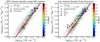 |
Fig. C.1. Left panel: comparison between ρSFR derived with the surface density of SNRs and the scale height of CCs (circles, as in Fig. 2) and ρSFR calculated with the surface density and the scale height of HII regions (squares). In both cases, ρgas is calculated with hydrostatic equilibrium (see Sect. 3.1). Right panel: comparison between ρgas derived with the hydrostatic equilibrium (circles, as in Fig. 2) and ρgas from different works in the literature (M17 = Marasco et al. 2017, BG78 = Burton & Gordon 1978, NS = Nakanishi & Sofue 2003, 2006), all with the ρSFR used in this work (see Sect. 3.2). In both panels, the symbols are colour-coded according to the Galactocentric radius, and the solid line and the red band show the VSF law and its intrinsic scatter derived for nearby disc galaxies, whose volume densities are represented by the grey contours containing, from lightest to darkest, 95%, 75%, 50%, and 25% of the points. |
In the right panel, we show different ρgas estimates taken from the exhaustive collection in Kramer & Randall (2016), who provide the volume densities of the atomic and the molecular gas by Burton & Gordon (1978) and Nakanishi & Sofue (2003, 2006) (the uncertainties are unfortunately not available), and from Marasco et al. (2017). All the points in Fig. C.1 are colour-coded according to the Galactocentric radius, and the spread in the points with the same colour (i.e. at the same R) can be interpreted as the uncertainty on the volume density measurements at that radius. We also show the volume densities of the sample of galaxies in B19 (grey contours) and the VSF law with slope α = 1.91 ± 0.03. The MW points are generally compatible with those of nearby galaxies and the VSF law, although the large scatter makes the comparison itself uncertain. The MW points derived without using the assumption of hydrostatic equilibrium seem to suggest a shallower slope (∼1.5) for the VSF law, but again the large uncertainties do not allow us to draw robust conclusions.
All Figures
|
Fig. 1. Scale height of CCs (data from Chen et al. 2019) as a function of the Galactocentric radius (black diamonds). The red curve is the gas scale height (Eq. (4)), i.e. the weighted average of the HI and the H2 scale heights. |
| In the text | |
|
Fig. 2. Correlations between the surface density (left) and the volume density (right) of the gas and the SFR in the MW, colour-coded according to the Galactocentric radius. The squares indicate measurements for R ≤ R⊙ from Marasco et al. (2017), while the circles are for R > R⊙ from Binney & Merrifield (1998), Nakanishi & Sofue (2003, 2006), and Levine et al. (2006) (see text). The grey points are the corresponding quantites for the sample of 12 nearby disc galaxies (see Figs. 5 and 6 in B19 for the whole range of densities). The solid line in the right panel is the VSF law from B19 with its intrinsic scatter (red band). |
| In the text | |
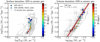 |
Fig. 3. Same as Fig. 2, but in this case the gas densities are for the atomic gas only. |
| In the text | |
 |
Fig. 4. Same as Fig. 2, but in this case the gas densities are for the molecular gas only. |
| In the text | |
|
Fig. A.1. Surface density radial profiles of the atomic gas (left), the molecular gas (centre), and the total gas (right) from the literature compared to the profile adopted in this work (black points). The factor 1.36 for the helium correction is included. Left panel: BG78 = Burton & Gordon (1978), Wo90 = Wouterloot et al. (1990), DL90 = Dickey & Lockman (1990), BM98 = Binney & Merrifield (1998), NS03 = Nakanishi & Sofue (2003), Le06 = Levine et al. (2006), KD08 = Kalberla & Dedes (2008), and M17 = Marasco et al. (2017). Centre panel: Sa84 = Sanders et al. (1984), Da87 = Dame et al. (1987), Gr87 = Grabelsky et al. (1987), Br88 = Bronfman et al. (1988), Cl88 = Clemens et al. (1988), Di91 = Digel (1991), Lu00 = Luna et al. (2006), NS06 = Nakanishi & Sofue (2006). |
| In the text | |
|
Fig. A.2. Scale height radial profiles of the atomic and molecular gas from the literature (Lo84 = Lockman 1984; see caption of Fig. A.1 for the other labels in the legend) compared to those calculated assuming the hydrostatic equilibrium (black points). |
| In the text | |
|
Fig. A.3. Volume density radial profiles of the atomic gas (left), the molecular gas (centre), and the total gas (right) from the literature (Li92 = Liszt 1992, KK98 = Kalberla & Kerp 1998, NS = HI from Nakanishi & Sofue 2003, and H2 from Nakanishi & Sofue 2006; see caption of Fig. A.1 for the other labels in the legend) compared to the profile adopted in this work (black points). The factor 1.36 for the helium correction is included. |
| In the text | |
|
Fig. B.1. Surface density (left panel) and scale height (right panel) of the SFR distribution using different tracers. The black points show the profile adopted in this work, while the others are different estimates from the literature (see text). The reference papers are indicated by the following abbreviations: L85 = Lyne et al. (1985), CB98 = Case & Bhattacharya (1998), YK04 = Yusifov & Küçük (2004), G15 = Green (2015), B00 = Bronfman et al. (2000), and L19 = Li et al. (2019). |
| In the text | |
|
Fig. C.1. Left panel: comparison between ρSFR derived with the surface density of SNRs and the scale height of CCs (circles, as in Fig. 2) and ρSFR calculated with the surface density and the scale height of HII regions (squares). In both cases, ρgas is calculated with hydrostatic equilibrium (see Sect. 3.1). Right panel: comparison between ρgas derived with the hydrostatic equilibrium (circles, as in Fig. 2) and ρgas from different works in the literature (M17 = Marasco et al. 2017, BG78 = Burton & Gordon 1978, NS = Nakanishi & Sofue 2003, 2006), all with the ρSFR used in this work (see Sect. 3.2). In both panels, the symbols are colour-coded according to the Galactocentric radius, and the solid line and the red band show the VSF law and its intrinsic scatter derived for nearby disc galaxies, whose volume densities are represented by the grey contours containing, from lightest to darkest, 95%, 75%, 50%, and 25% of the points. |
| In the text | |
Current usage metrics show cumulative count of Article Views (full-text article views including HTML views, PDF and ePub downloads, according to the available data) and Abstracts Views on Vision4Press platform.
Data correspond to usage on the plateform after 2015. The current usage metrics is available 48-96 hours after online publication and is updated daily on week days.
Initial download of the metrics may take a while.