| Issue |
A&A
Volume 632, December 2019
|
|
|---|---|---|
| Article Number | A103 | |
| Number of page(s) | 12 | |
| Section | Galactic structure, stellar clusters and populations | |
| DOI | https://doi.org/10.1051/0004-6361/201936431 | |
| Published online | 10 December 2019 | |
A MUSE study of the inner bulge globular cluster Terzan 9: a fossil record in the Galaxy⋆
1
Universidade de São Paulo, IAG, Rua do Matão 1226, Cidade Universitária, São Paulo 05508-900, Brazil
e-mail: This email address is being protected from spambots. You need JavaScript enabled to view it.
2
UK Astronomy Technology Centre, Royal Observatory, Blackford Hill, Edinburgh, EH9 3HJ, UK
3
IfA, University of Edinburgh, Royal Observatory, Blackford Hill, Edinburgh EH9 3HJ, UK
4
ESO, Alonso de Córdova 3107, Vitacura, Santiago, Chile
5
Departamento de Física, Facultad de Ciencias Exactas, Universidad Andrés Bello, Av. Fernandez Concha 700, Las Condes, Santiago, Chile
6
Astrophysics Research Institute, Liverpool John Moores University, 146 Brownlow Hill, Liverpool L3 5RF, UK
7
Universitá di Padova, Dipartimento di Fisica e Astronomia, Vicolo dell’Osservatorio 3, 35122 Padova, Italy
8
INAF-Osservatorio Astronomico di Padova, Vicolo dell’Osservatorio 5, 35122 Padova, Italy
9
Universidade Federal do Rio Grande so Sul, Departamento de Astronomia, Av. Bento Gonçalves 9500, Rio Grande do Sul, Brazil
10
Centre for Astrophysics and Supercomputing, Swinburne University of Technology, Hawthorn, VIC 3122, Australia
Received:
1
August
2019
Accepted:
14
October
2019
Abstract
Context. Moderately metal-poor inner bulge globular clusters are relics of a generation of long-lived stars that formed in the early Galaxy. Terzan 9, projected at 4°.12 from the Galactic center, is among the most central globular clusters in the Milky Way, showing an orbit which remains confined to the inner 1 kpc.
Aims. Our aim is the derivation of the cluster’s metallicity, together with an accurate measurement of the mean radial velocity. In the literature, metallicities in the range between −2.0 < [Fe/H] < −1.0 have been estimated for Terzan 9 based on color-magnitude diagrams and CaII triplet (CaT) lines.
Methods. Given its compactness, Terzan 9 was observed using the Multi Unit Spectroscopic Explorer (MUSE) at the Very Large Telescope. The extraction of spectra from several hundreds of individual stars allowed us to derive their radial velocities, metallicities, and [Mg/Fe]. The spectra obtained with MUSE were analysed through full spectrum fitting using the ETOILE code.
Results. We obtained a mean metallicity of [Fe/H] ≈ −1.10 ±0.15, a heliocentric radial velocity of vhr = 58.1 ± 1.1 km s−1, and a magnesium-to-iron [Mg/Fe] = 0.27 ± 0.03. The metallicity-derived character of Terzan 9 sets it among the family of the moderately metal-poor Blue Horizontal Branch clusters HP 1, NGC 6558, and NGC 6522.
Key words: stars: abundances / Galaxy: bulge / globular clusters: individual: Terzan 9
Based on observations collected at the European Organisation for Astronomical Research in the Southern Hemisphere, Paranal, Chile, under ESO programme 097.D-0093.
© ESO 2019
1. Introduction
Globular clusters in the central parts of the Galaxy are among the oldest extant stellar populations in the Milky Way (e.g. Barbuy et al. 2018a; Kunder et al. 2018). Terzan 9 is a very compact cluster located at 4 12 and 0.7 kpc (Bica et al. 2006) from the Galactic center, which is, thus, in the inner bulge volume, and it is among the globular clusters closest to the Galactic center. Terzan 9 appears to show a blue horizontal branch (BHB) in the ground-based color–magnitude diagrams (CMDs) by Ortolani et al. (1999). The clusters identified with a moderate metallicity and a BHB are very old as deduced from proper-motion cleaned color–magnitude diagrams (CMDs) for example for NGC 6522 and HP 1 (Kerber et al. 2018, 2019). A proper-motion cleaned CMD for Terzan 9 is presented in Rossi et al. (2015), with the cluster proper motions derived. Orbit calculations by Pérez-Villegas et al. (2018) reveal that Terzan 9 remains confined within 1 kpc of the Galactic center with an orbit co-rotating with the bar, it has a bar shape in the (x − y) projection, and a boxy shape in (x − z), which indicates that these clusters are trapped by the bar. With absolute proper motions from Gaia data release 2 (DR2), a new orbital analysis was carried out (Pérez-Villegas et al. 2020) using a Monte Carlo method to take into account the effect of the uncertainties in the observational parameters. These calculations confirm that Terzan 9 belongs to the bulge globular cluster group and that most of its probable orbits follow the bar. Since the bulge clusters are typically old, they were probably formed early in the Galaxy and were later trapped by the bar (see also Renzini et al. 2018). As a matter of fact, the bar should have formed at about 8 ± 2 Gyr ago, according to Buck et al. (2018).
A metallicity of [Fe/H] ∼ − 2.0 was deduced by Ortolani et al. (1999) and [Fe/H] ∼ − 1.2 by Valenti et al. (2007) from CMDs. Armandroff & Zinn (1988) obtained [Fe/H] = −0.99 from measurements of CaT lines. Vásquez et al. (2018; ESO proposal 089.D-0493) measured the CaT lines for six stars and obtained [Fe/H] ∼ − 1.08, −1.21, and −1.16 following calibrations from Dias et al. (2016), Saviane et al. (2012), and Vásquez et al. (2015), respectively. In the compilations by Harris (1996, edition of 2010)1 and Carretta et al. (2009), metallicities of [Fe/H] = −1.05 and −2.07 are respectively reported. Given that spectroscopic results are more reliable for metallicity derivations, it appears that a value of around [Fe/H] ∼ −1.0 should be preferred. The aim of this work is to obtain the metallicity derivation for Terzan 9, together with its radial velocity. The coordinates and typical photometric parameters for Terzan 9 are reported in Table 1.
Terzan 9: data from literature.
The ETOILE code (Katz et al. 2011; Dias et al. 2015) is used to derive the stellar parameters effective temperature, gravity, metallicity, and [Mg/Fe] ratio for each sample star. This code corrects for radial velocity, compares the observed spectra of a sample star to all spectra from a grid of spectra, and indicates which ones are the most similar. The procedure proved to work well, as demonstrated in Dias et al. (2015, 2016), where the method is applied to 800 red giants in 51 globular clusters, observed with FORS2 at a similar resolution as MUSE, which is of the order of R ∼ 2000 at 6000 Å.
In Sect. 2, we report our observations. In Sect. 3, the steps in data reduction are given. Extraction of stellar spectra and their analysis are given in Sect. 4. The results are discussed in Sect. 5. A summary is provided in Sect. 6.
2. Observations
Terzan 9 is faint and compact with a concentration factor of c = 2.50 and core radius rcore = 0.03′ (Harris 1996, updated in 2010), therefore the MUSE field of view (FoV) of 1′×1′ appears suitable to locate and identify a large number of member stars.
The input list of stars was created from a combination of the photometric observations of Ortolani et al. (1999) with the Danish telescope in 1998 and more recent observations with the NTT at ESO in 2012. The absolute calibration of the NTT 2012 data has been performed using our previous 1998 Danish data (Ortolani et al. 1999). About 800 stars in common between the Danish 1998 data and NTT 2012 have been matched and checked in order to transform the instrumental NTT magnitudes into the calibrated ones. Two almost linear relations in magnitude and colors have been found, with a residual slope, in a range within 0.01 mag, possibly due to minor linearity deviations mostly at magnitudes brighter than V < 16. A simple offset has been applied then to the instrumental magnitudes and colors. The formal error of the transformation in V and V − I is of about 0.025 mag for both. The photometric error is dominated by linearity deviations at faint magnitudes. The V and I data were calibrated with the following conversion coefficients:
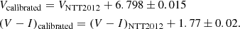
These two sets of data were combined in Rossi et al. (2015) and used for proper-motion decontamination, making use of the 14 yr time difference between the 1998 and 2012 observations to have an optimized selection of member stars. We transformed the original data given in pixels in X, Y into right ascension and declination (RA, Dec) based on the NTT 2012 image. The final coordinates are established by matching stars in common with the Gaia DR2 (Gaia Collaboration 2018). The list of stars with their coordinates, along with their V and V − I, are reported in Table A.1. In Fig. 1, we show an I image of Terzan 9 obtained at the NTT in 2012, with an excellent seeing of 0.5″.
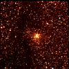 |
Fig. 1. Terzan 9: I image of Terzan 9 obtained at NTT in 2012, with seeing of 0.5 arcsec. Size is 2.2 × 2.2 arcmin2. |
The observations of the Terzan 9 field were conducted with the MUSE instrument installed on the UT4 Yepun unit of the Very Large Telescope (VLT), with the Wide Field Mode, no-AO, standard coverage (nominal mode WFM-NOAO-N). The FoV of MUSE in the Wide Field mode is 1′×1′ per exposure. The total observing time was 5 h including overheads, that were distributed along 5 observation blocks with 3 exposures (one in the central field and 2 offsets) of 948 s each. Besides a rotation of 90°, as recommended, and offsets of < 2 s in RA and of up to 18 s in Dec were applied. Detailed information about each exposure is given in Table 2. The MUSE datacubes were convolved with the transmission curves of the filters Red, Green and Blue, resulting in three images. The color composite image in B (4800 Å), V (5477 Å), and R (6349 Å) is shown in Fig. 2. We note that the Johnson-Cousins B filter overlaps only 22.77% of the MUSE wavelength coverage of 4800–9300 Å. That is the reason why the B in the color composite image, Fig. 2 is centered in 4800 Å instead of 4353 Å.
Observation log.
 |
Fig. 2. Terzan 9: composed image in B, V and R, from 5 different pointings of Terzan 9 obtained with MUSE on Yepun in 2016. Size is 1.1 × 1.1 arcmin2, exposures with seeing from 0.51″to 1.01″. |
3. Data reduction
3.1. Individual exposure reduction and sky subtraction
The individual exposures were reduced using the MUSE instrument pipeline v2.0.1 under the Reflex environment.
Since the field is highly crowded and reddened due to its location at low latitudes in the Galactic bulge, the sky subtraction must be carefully conducted. The MUSE pipeline gives the choice of the fraction of the FoV to be considered as sky. After some tests, we chose 6% based on the generated mask area, zones affected by sky contamination on the stellar spectra, and sky spectra comparisons assuming different fractions. For fractions much higher than 6%, the sky spectrum shows absorption lines of unresolved faint stars at redder wavelengths. For fractions much below 6% the final sky spectrum is not representative of the whole FoV, which implies that some sky-subtracted stellar spectra still show some sky emission lines.
The subtraction method used is simple, demonstrating a slight improvement in the signal-to-noise (S/N). Figures 3 (full wavelength range) and 4 (zoom on the bluest range) show the effect of sky subtraction. The faint sources are more affected by the sky than the bright ones because of their flux level being lower and closer to the sky level.
 |
Fig. 3. Comparison between sky contribution to bright and faint stellar sources. Spectra are normalized to their flux at 8604 Å. |
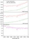 |
Fig. 4. Comparison between sky contribution to bright and faint stellar sources, normalized to their flux at 8604 Å. Scattered stellar light absorption lines can be seen in the sky spectrum, and its subtraction from the actual star spectrum preserves the true line profile. |
An example of spectra from different datacubes are shown in Fig. 6 for a sample star.
3.2. Datacube combination
The combination of the exposures was done by observation block (OB) using the most recent version (v2.1.1) of the MUSE instrument pipeline available only in the Gasgano environment. Gasgano’s interface allows for a quick assignment of frames to specific recipes and easy parameter manipulation, together with a processing request pool, so it is convenient for doing tests and requesting different datasets. We combined the three exposures of each OB to end up with five final cubes. The combination of all OBs was not done in the same way because they were observed in different conditions. The final stellar spectra correspond to the combination of the extracted 1D spectra of each star from the five cubes.
During the combination, several tests were carried out. The most influential parameter was the resampling method in building the combined cube. The MUSE pipeline default method is “drizzle” and comparisons between this method, along with other complex methods “renka” and “lanczos”, were performed. The renka method showed the best spatial resolution and image coverage among the three. We performed some tests with the renka resample method to find the critical radius cr value that optimizes the S/N of the extracted spectra, starting with the default value cr = 1.25. We noticed that the S/N increases for cr < 0.1 and that the line spread function (LSF) starts to degrade if we adopt cr < 0.03, therefore we chose cr = 0.03 to optimize the S/N of the extracted spectra without degrading the LSF. We also note that the reconstructed images using cr = 0.03 reveal fainter stars with a stable PSF and higher S/N, delivering a better result than with the default parameters2.
In addition, there were three other, simpler resampling methods: nearest, quadratic, and linear. A comparison between these three and the more complex methods discussed above showed that the linear method achieved even better results than “renka” both in terms of the S/N, and the spectral and spatial resolution. Our final resampling was done using the linear method. All of the comparisons were made visually with different source brightness in the regions of the Mg I triplet, Hα and Ca II triplet, as well as the spatial resolution and PSF quality, using DS9.
For each of the final cubes, 2D images were created by multiplying the cube by filters transmission curves available in the pipeline: Johnson B, V, Cousins R, I, and a few HST-ACS filters. These images were used to generate color–magnitude diagrams (CMDs) and select Red Giant Branch (RGB) stars to be cross-matched with our previous catalogue.
3.3. Extraction of stellar spectra
To extract the data from the MUSE datacubes, we employed the PampelMUSE3 code (Kamann et al. 2013) which is specific to stellar spectra extraction in crowded fields of data cubes such as MUSE. This software aptly deals with the observation of a densely populated stellar field such as a globular cluster. One challenge is the seeing-limited angular resolution of the instrument. A single object is represented by a point spread function (PSF), and the stellar field is a sum of many overlapping PSFs. Even in cases of heavily blended regions, the objects can be recovered using a PSF model if the distance between two neighbor stars is larger than 0.3 × FWHM.
This code written in python executes many tasks. In a simplified picture, a datacube is a sum of layers in wavelength of the image. A spaxel contains the entire spectrum, hence contributes to all layers. This method consists in analysing the datacube, layer by layer, performing PSF photometry individually on each layer. In the end all photometric solutions for each layer are combined, building spectra for each of the objects.
In order to get the spectra of sources of interest from the datacube, it is needed to provide an input catalogue with the position and magnitude of these objects, or else a selection by hand on the image. The coordinates are identified in the list of stars from the NTT 2012 observations (Sect. 2), and the proper motion cleaned CMDs by Rossi et al. (2015). The code locates the stars through a PSF fitting; a degree of confidence is assigned to each object, that can then be resolved in the crowded stellar field, and the spectra to be extracted.
To find a PSF in a crowded field, the program selects a number of relatively isolated objects and fits to them an analytical function. Then an Hermitian of order two is used to smooth the PSF parameters as a function of wavelength.
The last step in the data handling before the analysis is the removal of emission lines and non-stellar features left behind in the previous steps. These lines could introduce noise to the results in the minimum distance method which is the basis of the code ETOILE. The elimination of emission lines was made using a python code, which identifies the lines and cuts them in a region between their two edges, as illustrated in Fig. 5. We proceeded with the elimination of the emission line [O I] 5577.338 Å (Osterbrock et al. 1996) from all sample spectra. A future version of ETOILE may have the option of masking out undesired regions, such as those with their emission lines remaining after the cosmic ray cleaning and sky subtraction.
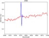 |
Fig. 5. Emission line subtraction from spectrum of star 2582. |
Finally, the extracted spectra for each star observed in different nights were combined to get a final 1D spectrum with higher S/N for each star. The combination is done following these steps: Fig. 6 shows the difference in flux levels in the spectra of a same star observed on different nights with the same exposure time but different weather conditions. We accounted for the difference in flux by normalizing them at 5000 Å and adding up all with no airmass-based or S/N-based weight, given that for the same star, there is little variation in S/N. S/N ∼ 110 for V ∼ 17, and S/N ∼ 90 for V ∼ 20. All S/N values are given in Table A.1.
 |
Fig. 6. Spectra of Terzan 9 star id 0072 from different data cubes obtained with PampelMUSE. |
4. Analysis
We derived atmospheric parameters via full spectrum fitting with the ETOILE code (Katz et al. 2011). This method is very robust in finding the absolute minimum in a χ2 map (e.g. Recio-Blanco 2014; Jofre et al. 2019). The code written in C is a modified version of the HALO (Cayrel et al. 1991) and TGMET (Katz et al. 1998) codes, which is obtained by changing the main four procedures: (a) the sample star spectrum is compared with the full list of reference spectra, (b) the input data are in ascii format, (c) the target spectrum does not need to be normalized or calibrated in absolute flux, and (d) no input parameters are given. More details on the method for extracting the fundamental stellar parameters (Teff, log g, [Fe/H]) from the spectra are given in Katz et al. (1998) and Katz (2001). In the original code, high resolution spectra of 2000 stars obtained with the ELODIE spectrograph, as presented in Katz et al. (2011), were adopted as reference.
Dias et al. (2015, 2016) implemented two other grids of spectra suitable for the analysis of medium-resolution spectra in the wavelength range 4600–5600 Å: the synthetic spectra by Coelho et al. (2005; hereafter Coelho05) and the MILES grid of observed spectra (Sánchez-Blásquez et al. 2006). We implemented a wavelength-extended version to be run with the Coelho05 library, encompassing the range 3000–18 000 Å that covers the region of the MUSE spectra of 4800–9300 Å, and it was used in different ways, as explained below.
In summary, the ETOILE code compares the observed spectrum to a list of reference spectra, either observed or synthetic, and finds the most similar ones through a least square of Euclidean distance measure. An example of a fit to a sample spectrum is given in Fig. 7.
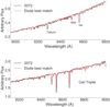 |
Fig. 7. Fit obtained with ETOILE for star 0072 with a good S/N = 129.80. Upper panel: region 6000–6800 Å where the strongest lines (telluric feature at 6282 Å, BaII 6496.9 Å and Hα) are indicated; lower panel: calcium triplet region. |
4.1. Sample extraction and radial velocities
We were able to extract and combine spectra from the five data cubes for 614 stars. After a selection based on S/N (S/N ≥ 85) of all final spectra, 90 of them were retained for analysis. The choice of this high S/N was due to better reliability in the parameter derivation. The ETOILE code was run for these spectra in order to derive their stellar parameters. The code first corrects for radial velocity (vr) through cross-correlation with a template spectrum from the library in use. In the present case, we used the MILES library in the wavelength range 4600–5600 Å, the synthetic Coelho05 library in the full MUSE range 4860–9300 Å, and in the region of the CaII triplet (CaT) 8400–8750 Å. The use of these different libraries and wavelength regions has shown that the most reliable method to derive radial velocities is the comparison of the sample spectra with the synthetic spectra in the CaT region. We concluded this from inspecting a series of spectra from the full initial sample and comparing them individually to reference spectra, verifying the wavelength region with that particular radial velocity value. The results are shown in Fig. 8 as smoothed histograms of radial velocities obtained in the three cases described above.
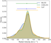 |
Fig. 8. Histograms of radial velocities obtained in the cases: green distribution: MILES library in the range 4860–5600 Å; blue distribution: Coelho05 library in the range 4860–9000 Å; and yellow distribution: Coelho05 library in the CaT region at 8400–8750 Å. |
Figure 9 shows the radial velocity distribution using the CaT region analysed through the Coelho05 library, for the 90 selected stars. A Gaussian fit results in a mean radial velocity value of vr = 49.7 km s−1 and a sigma of 22 km s−1. The mean heliocentric radial velocity is  km s−1. The radial velocity of
 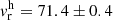 km s−1 from six stars by Vásquez et al. (2018) is compatible with the present value within uncertainties. A comparison with two stars in common with Vásquez et al. (2018) is reported in Table 3, showing excellent agreement in terms of radial velocities. In conclusion, we suggest that the present value is more accurate given the larger sample of stars taken into account.
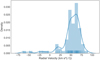 |
Fig. 9. Smoothed histogram of radial velocities obtained with the Coelho05 library in the CaT region at 8400–8750 Å. A kernel density estimation (KDE) Gaussian fitting the main peak of radial velocity distribution is overplotted. |
Comparison of radial velocity and metallicity for two stars in common with Vásquez et al. (2018, V+18).
For these two stars in common, the metallicities from the present work, derived with ETOILE and from CaT with the same method as Vásquez et al. (2018), that is, by applying their Eq. (5) for the metallicity scale by Dias et al. (2016) and their reported values, given in Table 3, show good agreement within uncertainties. The full explanation on how the metallicities are calibrated is given on Sect. 4.4.
Finally, the spectra are corrected for the adopted results of radial velocity, which are reported in Table A.2.
4.2. Coordinates and proper motions
The X, Y position of stars in the NTT image used to identify the stars in the MUSE data, were transformed to right ascension (RA) and declination (Dec) and matched with the Gaia DR2 (Gaia Collaboration 2018) coordinates, therefore the coordinate values reported in Table A.1 have a high astrometric precision. For the list of 90 selected stars, Gaia data are available.
In the MUSE field, there are 371 stars in the Gaia data that are shown in Fig. 10, where we see a clear cluster, seen as the feature highlighted in blue. Among the 371 Gaia stars, we identified 236 stars with proper motion (PM) information. For this sample, the mean proper motion values derived are: pmRA = −2.212 ± 0.0851 mas yr−1, and pmDec = −7.425 ± 0.0851 mas yr−1, in good agreement with derivations by Pérez-Villegas et al. (2020) of (−2.314 ± 0.108, −7.434 ± 0.068) mas yr−1 and (−2.225 ± 0.038, −7.492 ± 0.029) mas yr−1 from Vasiliev (2018). Note that the PM value derived uses 236 stars from Gaia which are present in the MUSE field. The values are the same as for the 90 selected member stars, as made evident in the corner plot given in Fig. 15. We note that the previous values by Rossi et al. (2015) of (0.0 ± 0.38, −3.07 ± 0.49) were different from these data, which are more accurate.
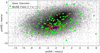 |
Fig. 10. Proper motions from Gaia. Symbols: gray dots: Gaia stars contained within a radius of 15 arcmin from the cluster center; Green dots: Gaia stars in a density representation enclosed in the MUSE field (1.1′×1.1′). The clustering of stars from Terzan 9 can be seen in red and blue, where blue is the densest part. |
In order to identify a final list of member stars, we selected stars within a certain range around the radial velocity of vr = 58.1 ± 1.1 km s−1, combined with proper motions of pmRA = −2.21 ± 0.10 and pmDec = −7.42 ± 0.07. We ended up with 67 stars, that are reported in Table A.1.
4.3. Stellar parameters
After radial velocity correction, the stellar spectrum is compared with the spectra of all stars in both libraries: Coelho05 and MILES. The ETOILE code ranks all spectra from the library by similarity (S) to the target spectrum. S is related to χ2, i.e., the most similar spectra have the smallest S value (for a definition of the similarity parameter, see Katz et al. 1998; Dias et al. 2015). A weighted mean of the stellar parameters Teff, log g, [Fe/H], and [α/Fe] of the most similar reference spectra is taken as the derived parameter of the target spectrum. The threshold to select the most similar spectra is based on the normalized similarity, S/S(1)≤1.1 (Dias et al. 2015), applied to results with both libraries.
The stellar parameters were first derived using the observed library MILES in the wavelength range of 4800–6000 Å, containing the MgI triplet lines, which is among the main features commonly used in spectra of galaxies (Mg2, Mgb, Fe5270, Fe5335, Faber et al. 1985). From this procedure we obtained our first set of results.
Using the Coelho05 library, we carried out tests in different spectral regions, as well as with the full spectral range of the MUSE spectra. As a check, we applied these calculations to spectra of the Sun, Arcturus and the metal-rich red giant μ Leo (Lecureur et al. 2007). For the synthesis of these spectra, the PFANT code (Barbuy et al. 2018b) was applied. The result indicated that the most reliable region is 6000–6800 Å, which is, in fact, the region commonly used to derive stellar parameters from high-resolution spectra (e.g. Barbuy et al. 2018c). This is explained by the following facts: it is widely known that when bluer than 6000 Å, the continuum is progressively affected by molecular lines as well as a large number of faint lines. When redder than 6800 Å, there are fewer lines, and, particularly fewer lines with well-defined oscillator strengths, and more numerous telluric lines. The stellar parameters were then derived by running ETOILE with the library Coelho05 in the range 6000–6800 Å, obtaining a second set of results.
From the final stellar parameters from the two applications (MILES and Coelho05), a mean metallicity obtained from ETOILE along with the two libraries is [Fe/H] = −1.12 ± 0.12, as shown in Fig. 11. It is important to note that there is a trend for lowering the metallicity as a function of lower S/N in this method. This is the reason for selecting only high S/N > 85 spectra; even so there is still a spread in metallicity values.
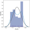 |
Fig. 11. Metallicity distribution of sample stars based on the optical analysis. The black curve represents a Gaussian fit centered at a mean value of [Fe/H] = −1.12 ± 0.12. The blue curve is a KDE Gaussian bandwidth estimated using Scott’s rule. |
Finally, in Fig. 14 the metallicity distribution vs. radial velocity distribution is shown, clearly indicating the locus of the cluster member stars. There is no strong correlation between the possible two peaks in metallicity hinted at in Fig. 11 and radial velocity, meaning that these are not two distinguished groups of similar metallicity and radial velocity values. In Fig. 15, the corner plot of different parameters of the member stars is given.
4.4. Uncertainties
The uncertainties in this paper regarding the stellar parameters are the same as those that have already been described in Sect. 3.2.2 in Dias et al. (2015). The uncertainties on the stellar parameters are computed using the average of squared residuals with the weighted 1/S2 as shown in the equation
 (1)
(1)
where par corresponds to the stellar parameters, Teff, log g, [Fe/H], and [α/Fe], and N is the number of stars. The m and M are counted as the number of the most similar stars in the library after the criteria of similarity S ≤ 1.1 is applied.
4.5. Metallicities from CaT
We normalized the NIR portion of the spectra around the CaT lines in order to perform the techniques described in Vásquez et al. (2015) and Vasiliev (2018). The two stronger lines (λλ 8542, 8662 Å) were fitted using a combination of a Gaussian and a Lorentzian profile, and the equivalent widths were summed (W = W8542 + W8662). Since we used the same script as in Vásquez et al. (2018), we were able to directly follow their calibrations, which we briefly describe here. The sum of the equivalent widths was first put into the same scale as Saviane et al. (2012) by applying the relation

The WS12 was then corrected by gravity and temperature effects by applying the correction, resulting into the reduced equivalent width

where VHB = 20.35 mag (Ortolani et al. 1999). The W′ was then converted into metallicity by applying the metallicity scale of Dias et al. (2016) represented by Eq. (5) of Vásquez et al. (2018), that is,
![Mathematical equation: $$ \begin{aligned} \mathrm{[Fe/H]}_{\rm D16} = 0.055 \times W{\prime }^{2} + 0.13 \times W\prime - 2.68. \end{aligned} $$](/articles/aa/full_html/2019/12/aa36431-19/aa36431-19-eq10.gif)
Example of CaT lines are shown in Fig. 12 for star 1378. A typical error in metallicity is of ±0.1 dex. The final list of cluster members where the metallicites derived from procedures using the ETOILE code and the CaT measurements are reported in Table A.2, which give a mean value of [Fe/H] = −1.09 ± 0.15, as shown in Fig. 13.
 |
Fig. 12. Fit to CaT lines A: 8498 Å; B: 8542 Å, and C: 8662 Å for star 1378 as example. The shaded gray areas show the local continuum regions and the shaded orange areas show the line region defined by Vásquez et al. (2015). The black lines and dots trace the observed spectrum in the rest frame and the blue lines are the best model fit to the data, using a sum of Gaussian and Lorentzian functions. The spectrum has been locally normalized using the highlighted local continuum regions before the fitting. In this analysis we only use the sum of the equivalent widths of the two strongest lines (B+C) following the recipe of Vásquez et al. (2015, 2018). |
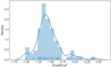 |
Fig. 13. Metallicity distribution of sample stars based on CaT analysis. |
Finally, a comparison of metallicities for the same stars from the ETOILE code and from CaT lines gives a mean difference of [Fe/H](ETOILE) – [Fe/H](CaT) ≈ −0.03 dex. In other words, from ETOILE we get a mean of [Fe/H] = −1.12 ± 0.12 and from CaT we get [Fe/H] = −1.09 ± 0.15, which are, therefore in excellent agreement.
Figure 14 shows the metallicity distribution vs. the radial velocity distribution for the identified 67 member stars. Figure 15 shows a corner plot relating metallicities, proper motions, and radial velocities.
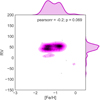 |
Fig. 14. Metallicity distribution based on optical analysis vs. radial velocity distribution, for identified member stars. |
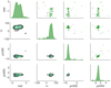 |
Fig. 15. Corner plot: metallicity, proper motion and radial velocities. |
4.6. Color–magnitude diagrams of member stars
In Fig. 16 we compare the I vs. V − I color–magnitude diagram showing all stars where the member stars are highlighted, and the resulting log g vs. Teff diagram. At the RGB base, a small trend towards high temperatures might be present. The brighter the RGB stars, the closer the isochrones get to the more metal-rich ones, again indicating that the metallicity is not bimodal and that the spread is due to S/N effects. On the right panel, member stars identified in the Gaia survey, are plotted with Gaia colors G vs. BR − RP. Dartmouth isochrones of 13 Gyr, [Fe/H] = −2.0 and [Fe/H] = −1.0 are overplotted. The I values were corrected by AI cf. Schlafly & Finkbeiner (2011)4; for the Gaia magnitudes no corrections were applied. In this figure we clearly see the RGB stars. A BHB appears more clearly present in Fig. 16b, confirming ealier evidence by Ortolani et al. (1999).
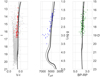 |
Fig. 16. I vs. V − I color–magnitude diagram showing all stars (gray) and member stars (red) (left panel), compared with the log g vs. Teff diagram (middle panel), and CMD in Gaia magnitudes and colors G vs. BP − RP for the stars in common (right panel). Dartmouth isochrones of 13 Gyr, and [Fe/H] = −1.0 are overplotted in black and isochrones of 13 Gyr, and [Fe/H] = −2.0 are overplotted in gray. |
5. Discussion
Photometric data indicate a broad range of metallicities: from V vs. V − I CMDs, Ortolani et al. (1999) deduced a metallicity of [Fe/H] ∼ −2.0, Valenti et al. (2007) instead derived [Fe/H] ∼ −1.2 from Ks vs. J − Ks CMDs; Bica et al. (1998) derived [Z/Z⊙]= − 1.01 from integrated spectra of CaT lines. High-resolution spectroscopic analyses based on CaT lines from the literature are available: Armandroff & Zinn (1988) obtained [Fe/H] = −0.99, and from 6 stars, Vásquez et al. (2018) report Fe/H] = −1.08 ± 0.14, −1.21 ± 0.15, −1.16 ± 0.21, on the scales of Dias et al. (2016), Saviane et al. (2012), and their own. The compilation by Harris (1996, 2010 edition) reports [Fe/H] = −1.05, whereas average metallicity compiled by Carretta et al. (2009), adopting a value from Harris (1996) from before 2010, was given as [Fe/H] = −2.07 ± 0.09. In the present work, the metallicity derived from the 67 selected member stars turned out to be of [Fe/H] = −1.12 ± 0.12 from the optical and [Fe/H] = −1.09 ± 0.15 from CaT lines, therefore, a final metallicity of [Fe/H] = −1.10 ± 0.15 was adopted.
The radial velocity of our sample stars was double-checked with synthetic spectra exhaustively, therefore, we suggest that our value of  km s−1 is more robust than the higher value of vr = 71.4 km s−1, given in Vásquez et al. (2018), due to the higher numbers of stars.
Terzan 9 is now included in the list of moderately metal-poor globular clusters with a BHB similar to HP 1 (Barbuy et al. 2016), NGC 6522 (Barbuy et al. 2014), and NGC 6558 (Barbuy et al. 2018c). Therefore, Terzan 4 continues, so far, to be the most metal-poor cluster in the Galactic bulge, with [Fe/H] = −1.6 (Origlia & Rich 2004). Other potential bulge clusters with metallicities below that of Terzan 4, and within 3.5 kpc from the Galactic center, specifically NGC 6144, NGC 6273, NGC 6287, NGC 6293, NGC 6293, NGC 6333, NGC 6541, are classified as halo intruders in Bica et al. (2016). The orbital classification by Pérez-Villegas et al. (2020) determines these clusters as inner/outer halo, thick disk or disk, and none of them are classified as a bulge member. As for NGC 6681, it has a radial velocity of 216.62 km s−1, and apogalactic distance of 4.97 kpc (Baumgardt et al. 2019), which might indicate that it is a halo intruder.
Terzan 9 has a blue HB, but not an extended one (see Ortolani et al. 1999). The moderately metal-poor metallicity found for Terzan 9 corresponds essentially to the lower end of the metallicity distribution of the bulk bulge stellar population. As a matter of fact, due to a fast chemical enrichment in the Galactic bulge, such as the one modeled by e.g. Cescutti et al. (2008), the iron abundance of [Fe/H] ∼ −1.3 is reached very fast, and stellar populations start to form in more significant numbers from there on, as confirmed by metallicity distribution functions (MDF) given in Zoccali et al. (2008, 2017), Hill et al. (2011), Ness et al. (2013), Rojas-Arriagada et al. (2014), Rojas-Arriagada & Recio-Blanco (2017) – see also Barbuy et al. (2018a).
The derivation of Mg-to-iron is based on the fitting of the MgI triplet lines (see Dias et al. 2015, 2016). In Fig. 17, the distribution of enhancement in the α-element Mg is shown with a mean value of [Mg/Fe] = +0.27 ± 0.03. The sigma of the distribution results is also ±0.03. This enhancement is similar to those reported in the Galactic bulge by Barbuy et al. (2018a) and Schultheis et al. (2017). This indicates that the stars in Terzan 9 were formed from gas resulting from an early fast chemical enrichment by core-collapse supernovae.
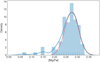 |
Fig. 17. Distribution in [Mg/Fe]. A KDE plot indicates a mean value of [Mg/Fe] = +0.27. |
6. Conclusions
We obtained MUSE datacubes for the bulge compact globular cluster Terzan 9. Using the software pampelMUSE by Kamann et al. (2013, 2018), we were able to extract the spectra of over 600 stars. The sample was reduced to 67 member stars by selecting spectra with S/N > 85 and with compatible radial velocities and proper motions. These spectra were analysed based on a full spectrum fitting with the ETOILE code in the area of 4600–5600 Å, compared with a grid of observed spectra (MILES, Sánchez-Blásquez et al. 2006). In the area of 6000–6800 Å, they were compared with a grid of synthetic spectra by Coelho et al. (2005; Coelh05). The CaT lines were also measured in order to obtain an independent derivation of metallicity. Both methods give very close mean results, with an adopted mean of [Fe/H] = −1.10 ± 0.15. This mean value is the outcome of the combination of a range of values where, in particular with regard to the optical region, two metallicity peaks are seen. In order to confirm metallicities, further observations with high resolution spectroscopy are of great interest. The present paper allows for a reliable target selection for such studies.
We were able to derive a mean heliocentric radial velocity of  km s−1, which is somewhat lower than the value from Vásquez et al. (2018) based on 6 stars, but the values are in agreement within uncertainties. These metallicities place Terzan 9 as a new member of the moderately metal-poor clusters with a blue horizontal branch that are found in the Galactic bulge.
Note that the MUSE pipeline developer Peter Weilbacher recommends the use of the standard pipeline.
Acknowledgments
We are grateful to David Katz for helpful comments on the Etoile code, and to Angeles Pérez-Villegas for help with the proper motion and orbital information. HE, BB, EB and EC acknowledge partial financial support, grants and fellowships from FAPESP, CNPq and CAPES – Finance code 001. HE and EC are grateful for their visit to ESO in Santiago, within ESO’s office for science programme, under supervision of B. Dias.
References
- Armandroff, T. E., & Zinn, R. 1988, A&AS, 140, 261 [Google Scholar]
- Barbuy, B., Chiappini, C., Cantelli, E., et al. 2014, A&A, 570, A76 [NASA ADS] [CrossRef] [EDP Sciences] [Google Scholar]
- Barbuy, B., Cantelli, E., Vemado, A., et al. 2016, A&A, 591, A53 [NASA ADS] [CrossRef] [EDP Sciences] [Google Scholar]
- Barbuy, B., Chiappini, C., & Gerhard, O. 2018a, ARA&A, 56, 223 [NASA ADS] [CrossRef] [Google Scholar]
- Barbuy, B., Trevisan, J., & de Almeida, A. 2018b, PASA, 35, 46 [NASA ADS] [CrossRef] [Google Scholar]
- Barbuy, B., Muniz, L., Ortolani, S., et al. 2018c, A&A, 619, A178 [NASA ADS] [CrossRef] [EDP Sciences] [Google Scholar]
- Bica, E., Claria, J. J., Piatti, A. E., & Bonatto, C. 1998, A&AS, 131, 483 [NASA ADS] [CrossRef] [EDP Sciences] [Google Scholar]
- Bica, E., Bonatto, C., Barbuy, B., & Ortolani, S. 2006, A&A, 450, 105 [NASA ADS] [CrossRef] [EDP Sciences] [Google Scholar]
- Bica, E., Ortolani, S., & Barbuy, B. 2016, PASA, 33, 28 [Google Scholar]
- Baumgardt, H., Hilker, M., Sollima, A., & Bellini, A. 2019, MNRAS, 482, 5138 [Google Scholar]
- Buck, T., Ness, M., Macciò, A. V., Obreja, A., & Dutton, A. A. 2018, ApJ, 861, 88 [NASA ADS] [CrossRef] [Google Scholar]
- Cayrel, R., Perrin, M. N., Barbuy, B., & Buser, R. 1991, A&A, 247, 108 [NASA ADS] [Google Scholar]
- Carretta, E., Bragaglia, A., Gratton, R., D’Orazi, V., & Lucatello, S. 2009, A&A, 508, 695 [NASA ADS] [CrossRef] [EDP Sciences] [Google Scholar]
- Cescutti, G., Matteucci, F., Lanfranchi, G. A., & McWilliam, A. 2008, A&A, 491, 401 [NASA ADS] [CrossRef] [EDP Sciences] [Google Scholar]
- Coelho, P., Barbuy, B., Meléndez, J., Schiavon, R. P., & Castilho, B. V. 2005, A&A, 443, 735 [NASA ADS] [CrossRef] [EDP Sciences] [Google Scholar]
- Dias, B., Barbuy, B., Saviane, I., et al. 2015, A&A, 573, A13 [NASA ADS] [CrossRef] [EDP Sciences] [Google Scholar]
- Dias, B., Barbuy, B., Saviane, I., et al. 2016, A&A, 590, A9 [NASA ADS] [CrossRef] [EDP Sciences] [Google Scholar]
- Faber, S. M., Friel, E., Burstein, D., & Gaskell, C. M. 1985, ApJ, 57, 711 [Google Scholar]
- Gaia Collaboration (Brown, A. G. A., et al.) 2018, A&A, 616, A1 [NASA ADS] [CrossRef] [EDP Sciences] [Google Scholar]
- Harris, W. 1996, AJ, 112, 1487 [NASA ADS] [CrossRef] [Google Scholar]
- Hill, V., Lecureur, A., Gómez, A., et al. 2011, A&A, 534, A80 [NASA ADS] [CrossRef] [EDP Sciences] [Google Scholar]
- Jofre, O., Heiter, U., & Soubiran, C. 2019, ARA&A, 57, 571 [NASA ADS] [CrossRef] [Google Scholar]
- Kamann, S., Wisotzki, L., & Roth, M. M. 2013, A&A, 549, A71 [NASA ADS] [CrossRef] [EDP Sciences] [Google Scholar]
- Kamann, S., Husser, T.-O., Dreizler, S., et al. 2018, MNRAS, 473, 5591 [NASA ADS] [CrossRef] [Google Scholar]
- Katz, D. 2001, J. Astron. Data, 7, 8 [Google Scholar]
- Katz, D., Soubiran, C., Cayrel, R., Adda, M., & Cautain, R. 1998, A&A, 338, 151 [NASA ADS] [Google Scholar]
- Katz, D., Soubiran, C., Cayrel, R., et al. 2011, A&A, 525, A90 [NASA ADS] [CrossRef] [EDP Sciences] [Google Scholar]
- Kerber, L. O., Nardiello, D., Ortolani, S., et al. 2018, ApJ, 853, 15 [NASA ADS] [CrossRef] [Google Scholar]
- Kerber, L. O., Libralato, M., Ortolani, S., et al. 2019, MNRAS, 484, 5530 [NASA ADS] [CrossRef] [Google Scholar]
- Kunder, A., Valenti, E., Dall’Ora, M., et al. 2018, Space Sci. Rev., 214, 90 [NASA ADS] [CrossRef] [Google Scholar]
- Lecureur, A., Hill, V., Zoccali, M., et al. 2007, A&A, 465, 799 [NASA ADS] [CrossRef] [EDP Sciences] [Google Scholar]
- Ness, M., Freeman, K., Athanassoula, E., et al. 2013, MNRAS, 430, 836 [NASA ADS] [CrossRef] [Google Scholar]
- Origlia, L., & Rich, R. M. 2004, AJ, 127, 3422 [NASA ADS] [CrossRef] [Google Scholar]
- Ortolani, S., Bica, E., & Barbuy, B. 1999, A&AS, 138, 267 [NASA ADS] [CrossRef] [EDP Sciences] [Google Scholar]
- Osterbrock, D. E., Fulbright, J. P., Martel, A. R., et al. 1996, PASP, 108, 277 [NASA ADS] [CrossRef] [Google Scholar]
- Pérez-Villegas, A., Rossi, L., Ortolani, S., et al. 2018, PASA, 35, 21 [Google Scholar]
- Pérez-Villegas, A., Barbuy, B., Kerber, L., et al. 2020, MNRAS, in press [arXiv:1911.05207] [Google Scholar]
- Recio-Blanco, A. 2014, IAU Symp., 298, 366 [NASA ADS] [Google Scholar]
- Renzini, A., Gennaro, M., Zoccali, M., et al. 2018, ApJ, 863, 16 [NASA ADS] [CrossRef] [Google Scholar]
- Rojas-Arriagada, A., Recio-Blanco, A., Hill, V., et al. 2014, A&A, 569, A103 [NASA ADS] [CrossRef] [EDP Sciences] [Google Scholar]
- Rojas-Arriagada, A., Recio-Blanco, A., de Laverny, P., et al. 2017, A&A, 601, A140 [NASA ADS] [CrossRef] [EDP Sciences] [Google Scholar]
- Rossi, L., Ortolani, S., Bica, E., Barbuy, B., & Bonfanti, A. 2015, MNRAS, 450, 3270 [NASA ADS] [CrossRef] [Google Scholar]
- Sánchez-Blásquez, P., Peletier, R. F., Jiménez-Vicente, J., et al. 2006, MNRAS, 371, 703 [NASA ADS] [CrossRef] [Google Scholar]
- Saviane, I., da Costa, G. S., Held, E. V., et al. 2012, A&A, 540, A27 [NASA ADS] [CrossRef] [EDP Sciences] [Google Scholar]
- Schlafly, E., & Finkbeiner, D. P. 2011, ApJ, 737, 103 [NASA ADS] [CrossRef] [Google Scholar]
- Schultheis, M., Rojas-Arriagada, A., García-Pérez, A., et al. 2017, A&A, 600, A14 [NASA ADS] [CrossRef] [EDP Sciences] [Google Scholar]
- Valenti, E., Ferraro, F. R., & Origlia, L. 2007, AJ, 133, 1287 [NASA ADS] [CrossRef] [Google Scholar]
- Vásquez, S., Zoccali, M., Hill, V., et al. 2015, A&A, 580, A121 [NASA ADS] [CrossRef] [EDP Sciences] [Google Scholar]
- Vásquez, S., Saviane, I., Held, E. V., et al. 2018, A&A, 619, A13 [NASA ADS] [CrossRef] [EDP Sciences] [Google Scholar]
- Vasiliev, E. 2018, MNRAS, 484, 2832 [Google Scholar]
- Zoccali, M., Hill, V., Lecureur, A., et al. 2008, A&A, 486, 177 [NASA ADS] [CrossRef] [EDP Sciences] [Google Scholar]
- Zoccali, M., Vásquez, S., Gonzalez, O. A., et al. 2017, A&A, 599, A12 [NASA ADS] [CrossRef] [EDP Sciences] [Google Scholar]
Appendix A: Extracted stars from the MUSE datacubes
Identified member stars from MUSE datacubes selected with S/N > 85.
Identified members stars from MUSE datacubes selected with S/N > 85.
All Tables
Comparison of radial velocity and metallicity for two stars in common with Vásquez et al. (2018, V+18).
All Figures
|
Fig. 1. Terzan 9: I image of Terzan 9 obtained at NTT in 2012, with seeing of 0.5 arcsec. Size is 2.2 × 2.2 arcmin2. |
| In the text | |
|
Fig. 2. Terzan 9: composed image in B, V and R, from 5 different pointings of Terzan 9 obtained with MUSE on Yepun in 2016. Size is 1.1 × 1.1 arcmin2, exposures with seeing from 0.51″to 1.01″. |
| In the text | |
|
Fig. 3. Comparison between sky contribution to bright and faint stellar sources. Spectra are normalized to their flux at 8604 Å. |
| In the text | |
|
Fig. 4. Comparison between sky contribution to bright and faint stellar sources, normalized to their flux at 8604 Å. Scattered stellar light absorption lines can be seen in the sky spectrum, and its subtraction from the actual star spectrum preserves the true line profile. |
| In the text | |
|
Fig. 5. Emission line subtraction from spectrum of star 2582. |
| In the text | |
|
Fig. 6. Spectra of Terzan 9 star id 0072 from different data cubes obtained with PampelMUSE. |
| In the text | |
|
Fig. 7. Fit obtained with ETOILE for star 0072 with a good S/N = 129.80. Upper panel: region 6000–6800 Å where the strongest lines (telluric feature at 6282 Å, BaII 6496.9 Å and Hα) are indicated; lower panel: calcium triplet region. |
| In the text | |
|
Fig. 8. Histograms of radial velocities obtained in the cases: green distribution: MILES library in the range 4860–5600 Å; blue distribution: Coelho05 library in the range 4860–9000 Å; and yellow distribution: Coelho05 library in the CaT region at 8400–8750 Å. |
| In the text | |
|
Fig. 9. Smoothed histogram of radial velocities obtained with the Coelho05 library in the CaT region at 8400–8750 Å. A kernel density estimation (KDE) Gaussian fitting the main peak of radial velocity distribution is overplotted. |
| In the text | |
|
Fig. 10. Proper motions from Gaia. Symbols: gray dots: Gaia stars contained within a radius of 15 arcmin from the cluster center; Green dots: Gaia stars in a density representation enclosed in the MUSE field (1.1′×1.1′). The clustering of stars from Terzan 9 can be seen in red and blue, where blue is the densest part. |
| In the text | |
|
Fig. 11. Metallicity distribution of sample stars based on the optical analysis. The black curve represents a Gaussian fit centered at a mean value of [Fe/H] = −1.12 ± 0.12. The blue curve is a KDE Gaussian bandwidth estimated using Scott’s rule. |
| In the text | |
|
Fig. 12. Fit to CaT lines A: 8498 Å; B: 8542 Å, and C: 8662 Å for star 1378 as example. The shaded gray areas show the local continuum regions and the shaded orange areas show the line region defined by Vásquez et al. (2015). The black lines and dots trace the observed spectrum in the rest frame and the blue lines are the best model fit to the data, using a sum of Gaussian and Lorentzian functions. The spectrum has been locally normalized using the highlighted local continuum regions before the fitting. In this analysis we only use the sum of the equivalent widths of the two strongest lines (B+C) following the recipe of Vásquez et al. (2015, 2018). |
| In the text | |
|
Fig. 13. Metallicity distribution of sample stars based on CaT analysis. |
| In the text | |
|
Fig. 14. Metallicity distribution based on optical analysis vs. radial velocity distribution, for identified member stars. |
| In the text | |
|
Fig. 15. Corner plot: metallicity, proper motion and radial velocities. |
| In the text | |
|
Fig. 16. I vs. V − I color–magnitude diagram showing all stars (gray) and member stars (red) (left panel), compared with the log g vs. Teff diagram (middle panel), and CMD in Gaia magnitudes and colors G vs. BP − RP for the stars in common (right panel). Dartmouth isochrones of 13 Gyr, and [Fe/H] = −1.0 are overplotted in black and isochrones of 13 Gyr, and [Fe/H] = −2.0 are overplotted in gray. |
| In the text | |
|
Fig. 17. Distribution in [Mg/Fe]. A KDE plot indicates a mean value of [Mg/Fe] = +0.27. |
| In the text | |
Current usage metrics show cumulative count of Article Views (full-text article views including HTML views, PDF and ePub downloads, according to the available data) and Abstracts Views on Vision4Press platform.
Data correspond to usage on the plateform after 2015. The current usage metrics is available 48-96 hours after online publication and is updated daily on week days.
Initial download of the metrics may take a while.