| Issue |
A&A
Volume 631, November 2019
|
|
|---|---|---|
| Article Number | A113 | |
| Number of page(s) | 15 | |
| Section | Stellar atmospheres | |
| DOI | https://doi.org/10.1051/0004-6361/201936343 | |
| Published online | 01 November 2019 | |
Abundances of disk and bulge giants from high-resolution optical spectra
IV. Zr, La, Ce, Eu★,★★
1
Lund Observatory, Department of Astronomy and Theoretical Physics, Lund University,
Box 43,
221 00
Lund,
Sweden
e-mail: This email address is being protected from spambots. You need JavaScript enabled to view it.
2
Materials Science and Applied Mathematics, Malmö University,
205 06
Malmö,
Sweden
3
Université Côte d’Azur, Observatoire de la Côte d’Azur, CNRS, Laboratoire Lagrange, Bd de l’Observatoire,
CS 34229,
06304
Nice Cedex 4,
France
4
Dipartimento di Fisica, Sezione di Astronomia, Università di Trieste,
via G.B. Tiepolo 11,
34131
Trieste,
Italy
5
INAF – Osservatorio Astronomico di Trieste,
via G.B. Tiepolo 11,
34131
Trieste,
Italy
6
INFN – Sezione di Trieste,
via Valerio 2,
34134
Trieste,
Italy
Received:
18
July
2019
Accepted:
18
September
2019
Abstract
Context. Observations of the Galactic bulge suggest that the disk formed through secular evolution rather than gas dissipation and/or mergers, as previously believed. This would imply very similar chemistry in the disk and bulge. Some elements, such as the α-elements, are well studied in the bulge, but others like the neutron-capture elements are much less well explored. Stellar mass and metallicity are factors that affect the neutron-capture process. Due to this, the enrichment of the ISM and the abundance of neutron-capture elements vary with time, making them suitable probes for Galactic chemical evolution.
Aims. In this work, we make a differential comparison of neutron-capture element abundances determined in the local disk(s) and the bulge, focusing on minimising possible systematic effects in the analysis, with the aim of finding possible differences/similarities between the populations.
Methods. Abundances are determined for Zr, La, Ce, and Eu in 45 bulge giants and 291 local disk giants, from high-resolution optical spectra. The abundances are determined by fitting synthetic spectra using the SME-code. The disk sample is separated into thin- and thick-disk components using a combination of abundances and kinematics.
Results. We find flat Zr, La, and Ce trends in the bulge, with a ~0.1 dex higher La abundance compared with the disk, possibly indicating a higher s-process contribution for La in the bulge. [Eu/Fe] decreases with increasing [Fe/H], with a plateau at around [Fe/H] ~−0.4, pointing at similar enrichment to α-elements in all populations.
Conclusions. We find that the r-process dominated the neutron-capture production at early times both in the disks and bulge. Further, [La/Eu] ratios for the bulge are systematically higher than for the thick disk, pointing to either a) a different amount of SN II or b) a different contribution of the s-process in the two populations. Considering [(La+Ce)/Zr], the bulge and the thick disk follow each other closely, suggesting a similar ratio of high-to-low-mass asymptotic giant branch stars.
Key words: stars: abundances / Galaxy: bulge / solar neighborhood / Galaxy: evolution
Full Tables A.1–A.4 are only available at the CDS via anonymous ftp to cdsarc.u-strasbg.fr (130.79.128.5) or via http://cdsarc.u-strasbg.fr/viz-bin/cat/J/A+A/631/A113
Based on observations made with the Nordic Optical Telescope (programs 51-018 and 53-002) operated by the Nordic Optical Telescope Scientific Association at the Observatorio del Roque de los Muchachos, La Palma, Spain, of the Instituto de Astrofisica de Canarias, spectral data retrieved from PolarBase at Observatoire Midi Pyrénées, and observations collected at the European Southern Observatory, Chile (ESO programs 71.B-0617(A), 073.B-0074(A), and 085.B-0552(A)).
© ESO 2019
1 Introduction
Our view of the structure and formation of the Galactic bulge has changed dramatically over the past decade. Earlier, the prevailing view was that the bulge is a spheroid in a disk formed in an early, rapid, dissipative collapse (e.g. Immeli et al. 2004), naturally resulting from major mergers for example, converting disks to classical bulges (e.g. Shen & Li 2016). However, with new findings and an accumulation of data, what we call the bulge is today predominately considered to be mainly the inner structures of the Galactic bar seen edge-on (e.g. Portail et al. 2017). The details of its structure and timescales for its formation are nevertheless unclear (e.g. Barbuy et al. 2018).
Metallicity distributions and abundance-ratio trends with metallicity provide important means to determine the evolution of stellar populations, also in the bulge. Trends of different element groups formed in different nucleosynthetic channels provide strong complementary constraints. Also, comparisons of trends between different stellar populations, for example the local thick disk, can be used to constrain the history of the bulge. Whether or not there is an actual difference in abundance trends with metallicity between the bulge and the local thick disk is unclear (McWilliam 2016; Barbuy et al. 2018; Zasowski et al. 2019; Lomaeva et al. 2019). Some elements such as Sc, V, Cr, Co, Ni, and Cu show differences in some investigations, whereas others show great similarities. New abundance studies minimising systematic uncertainties are clearly needed.
An important nucleosynthetic channel that has not yet been thoroughly investigated in the bulge is that of the heavy elements, namely the neutron-capture elements. These can be divided into two groups: the slow (s)- and rapid (r)-process elements, depending on the timescales between the subsequent β-decay and that of the interacting neutron flux (Burbidge et al. 1957). The neutron flux in the s-process is such that the timescale of interaction is slower than the subsequent β-decay, making the elements created in this process stable and generally found in the so-called valley of stability, whilst it is the other way around for the r-process, resulting in the creation of heavier elements. As a point of reference, the s-process therefore produces the lighter elements after iron (A ≥ 60), whereasthe r-process is the dominating production process for the heaviest elements. Nonetheless, it is important to keep in mind that the production of heavier elements is a combination of the two processes and an “s- or r-process element” simply refers to an element with a dominating contribution from one of the processes. The neutron densities required for the s- and r-processes are ≤ 107 −1015 cm−3 (Busso et al. 1999; Karakas & Lattanzio 2014) and somewhere between 1024 −1028 cm−3 (Kratz et al. 2007), respectively, putting some constraints on the astrophysical sites where they can occur.
The s-process can in turn be divided into three sub-processes: the weak, main and strong s-processes taking place in massive stars (weak)and asymptotic giant branch (AGB) stars (main, strong). Furthermore, the s-process elements can be divided into the light, heavy, and very heavy s-process elements, the naming originating from their atomic masses of A = 90, 138 and 208 (around Zr, La, and Pb, respectively). A build-up is created at these stable nuclei (N = 50, 82, and 126, also known as magic numbers) due to isotopes with low neutron cross sections, creating bottlenecks in the production of heavier elements and in turn, peaks of stable isotopes. Thus, the naming first- second-, and third-peak s-process is often also used for the light, heavy and very heavy s-process elements. In this work, light and heavy s-process elements produced in the main s-process will be analysed (Zr, La, Ce).
The main s-process takes place in the interior of low- and intermediate-mass AGB stars (Herwig 2005; Karakas & Lattanzio 2014) with the neutrons originating from the reactions  and
and  . The second reaction takes place at higher temperatures in AGB stars with initial masses of > 4 M⊙. The process takes place in the so-called 13C-pocket in between the hydrogen and helium burning shells during the third dredge-up (TDU; Bisterzo et al. 2017). Since AGB stars have an onset delay on cosmic scales, a non-negligible fraction of the s-process-dominated elements is likely to originate from the r-process at early times. Furthermore, the light s-process elements (first-peak s-process) can have a possible production from the weak s-process, taking place in helium core burning and in the subsequent convective carbon-burning-shell phase in massive stars (Couch et al. 1974). However, previous observations cannot fully explain the abundance of the light s-process elements at early times, and other possible origins have therefore been proposed (e.g. LEPP; Travaglio et al. 2004; Cristallo et al. 2015).
The production site(s) for r-process elements is yet to be constrained, but the proposed sites are various neutron-rich (violent) events, such as core-collapse supernovae (CC SNe), collapsars, and the mergers of heavy bodies in binaries, such as neutron star mergers (Sneden et al. 2000; Thielemann et al. 2011, 2017). The electromagnetic counterpart to the observed neutron merger GW170817 (Abbott et al. 2017) indeed showed r-process elements. Research is still ongoing to determine whether or not neutron star mergers are the only, or even the dominating, source of r-process elements (e.g. Thielemann et al. 2018; Côté et al. 2019; Siegel et al. 2019; Kajino et al. 2019).
In order to put constraints on the neutron capture yields, it is important to have reliable observational abundances to compare with the models. In the review paper on the chemical evolution of the bulge by McWilliam (2016), the necessity of having properly measured abundances for the disk in order to have a reference sample for bulge measurements is stressed, and these are provided in this work.
Regarding the determination of neutron-capture elements in bulge stars, such analyses have been made previously by Johnson et al. (2012), Van der Swaelmen et al. (2016), and Duong et al. (2019). Johnson et al. (2012) studied stars in Plaut’s field (b = −8°) observed with the Hydra multifibre spectrograph at the Blanco 4m telescope, determining the abundances of Zr, La, Nd, and Eu. Their [La/Fe] trend versus metallicity of the stars in the bulge field is clearly different from that of the thick disk. These latter authors therefore concluded that the metal-poor bulge, or the inner disk, is likely chemically different from that of the thick disk. Van der Swaelmen et al. (2016) studied Ba, La, Ce, Nd and Eu in 56 Galactic bulge giants observed with FLAMES/UVES at the VLT, finding that the s-process elements Ba, La, Ce, and Nd have decreasing [Ba,La,Ce,Nd/Fe] abundances with increasing metallicity, separating them from the flatter thick-disk trends. Additionally, in the work by Duong et al. (2019), Zr, La, Ce, Nd and Eu are measured for a large bulge sample at latitudes of b = −10°, − 7.5° and − 5°, observed with the HERMES spectrograph on the Anglo-Australian Telescope. These latter authors find indications of the bulge having a higher star formation rate than that of the disk.
Johnson et al. (2012) and Van der Swaelmen et al. (2016) compare their bulge abundances with previously determined disk abundances, mainly from dwarf stars, which might obstruct the interpretation of the comparative abundances due to the risk of systematic uncertainties between analyses of dwarf and giant stars1. Previous studies by Meléndez et al. (2008) and Gonzalez et al. (2015) stressed the importance of comparing stars within the same evolutionary stage. Furthermore, in investigations of atomic diffusion and mixing in stars (Korn et al. 2007; Lind et al. 2008; Nordlander et al. 2012; Gruyters et al. 2016; Souto et al. 2019; Liu et al. 2019), it has been shown that dwarf stars might have systematically lower elemental abundances compared to evolved stars, suggesting that abundances measured from dwarf stars are too low. The magnitude of this depletion is measurable and should, in general, be considered for the relevant elements in order to properly probe the Galactic composition and its evolution based on dwarf stars.
In this paper, we study the four neutron-capture elements Zr, La, Ce, and Eu determined from optical spectra of giants observed with FLAMES/UVES for the bulge sample. We compare the obtained abundance-ratio trends with that of the local disk obtained from a comparison sample of similarly analysed giants (observed with FIES at high resolution in the same wavelength range). Section 2 describe the bulge and disk samples. The same methodology for determining the stellar parameters and abundances (a carefully chosen set of spectral lines) ensures a minimisation of the systematic uncertainties in the comparison of the two samples, following the same methodology as the previous papers in this series; Jönsson et al. (2017a,b); Lomaeva et al. (2019), see Sect. 3. We present the results in Sect. 4 and discuss these in Sect. 5.
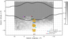 |
Fig. 1 Map of the Galactic bulge showing the five analysed fields (SW, B3, BW, B6, and BL). The bulge samples from Johnson et al. (2012), Van der Swaelmen et al. (2016), and Duong et al. (2019) are also marked in the figure. The dust extinction towards the bulge is taken from Gonzalez et al. (2011, 2012) and scaled to optical extinction (Cardelli et al. 1989). The scale saturates at AV = 2, which is the upper limit in the figure. The COBE/DIRBE contours of the Galactic bulge, in black, are from Weiland et al. (1994). |
2 Observations
2.1 Bulge sample
Since large amounts of dust lies in the line of sight towards the Galactic centre resulting in a high optical extinction, observing bulge stars can be challenging at optical wavelengths. Our ambition was to include fields as close to the centre of the bulge as possible, whilst keeping to regions where the extinction is manageable.
The Galactic bulge sample consists of 45 giants (see Table A.1). The spectra were obtained using the spectrometer FLAMES/UVES mounted on the VLT, Chile, observed in May-August 2003-2004. Twenty-seven of these spectra were also analysed in Van der Swaelmen et al. (2016). In addition to these, 18 spectra from the Sagittarius Window, (l, b) = (1.29°, −2.65°), lying closer to the Galactic plane in a region with relatively low extinction, are added to the sample analysed here. These were observed in August 2011 (ESO programme 085.B-0552(A)). In total, five bulge fields are included in the bulge sample: SW (the Sagittarius Window), BW (Baade’s Window), BL (the Blanco field), B3, and B62. The fields can beseen in Fig. 1, overlaid on an optical extinction map, together with the fields analysed in Johnson et al. (2012) and Duong et al. (2019). From Fig. 1 one can see that the SW field lies in a region of relatively low extinction and closer to the Galactic plane than the other fields.
The FLAMES/UVES instrument allows for simultaneous observation of up to seven stars. Depending on the extinction and local conditions, each setting in our observations required an integration time of somewhere between 5 and 12 h. The achieved signal-to-noise ratios (S/N) of the recorded bulge spectra are between 10 and 80. The resolving power of the spectra is R ~ 47 000 and the usable wavelength coverage is limited to the range 5800–6800 Å.
The distances to our bulge stars are estimated to range between 4 and 12 kpc from the solar system (Bailer-Jones et al. 2018), placing the stars within the Galactic regions classified as the bulge by Wegg et al. (2015). Although it should be noted that distance estimation can be rather troublesome and Gaia DR2 (Gaia Collaboration 2016, 2018) reports a parallax uncertainty higher than 20% for the majority of our bulge stars.
2.2 Disk sample
The disk sample consists of 291 giants stars, a majority of these placed within 2 kpc of the solar system (see Table A.2). The bulk of the sample is observed at the Nordic Optical Telescope (NOT), La Palma, using the FIbre-fed Echelle Spectrograph (FIES; Telting et al. 2014), under the programme 51-018 (150 stars) in May–June 2015 and 53-002 (63 stars) in June 2016. Forty-one spectra were taken from the stellar sample in Thygesen et al. (2012), also observed using the FIES at the NOT. An additional 18 spectra were downloaded from the FIES archive. Lastly, 19 spectra were taken from the PolarBase data base (Petit et al. 2014) where NARVAL and ESPaDOnS were used (mounted on Telescope Bernard Lyot and Canada–France–Hawaii Telescope, respectively). The FIES and PolarBase have similar resolving powers of R ~ 67 000 and R ~ 65 000, respectively.
All three spectrometers cover wide regions in the optical domain, but in order to maximise the coherency in this work, the wavelength region used is restricted to that of the bulge spectra: 5800–6800 Å. The resulting S/N of the FIES spectra are around 80–120 per data point in the reduced spectrum. Similar values can be found for the PolarBase spectra whereas the Thygesen et al. (2012) spectra have a lower S/N of about 30–50. Details of how the S/N was calculated can be found in Jönsson et al. (2017a).
The reduction of the FIES spectra was preformed using the standard FIES pipeline and the Thygesen et al. (2012) and PolarBase data was already reduced. A crude normalisation of all spectra was done initially with the IRAF task continuum. Later in the analysis, the continuum is re-normalised more carefully by a manual placement of continuum regions and subsequently fitting a straight line to these, allowing a higher precision of the abundance determination (more on this in Sect. 3.3).
Telluric lines have not been removed from the spectra. Instead a telluric spectrum from the Arcturus atlas (Hinkle et al. 2000) has been plotted over the appropriately shifted observed spectra and affected regions have been avoided on a star-by-star basis.
3 Analysis
The analysis of the spectra and the determination of the stellar abundances follows the same methodology as described in the previous papers in this series: Jönsson et al. (2017a,b) and Lomaeva et al. (2019). This section describes the general methodology as well as the specific details relevant for this work.
3.1 General methodology
To determine the stellar abundances, synthetic spectra are modelled using the tool Spectroscopy Made Easy (SME, Valenti & Piskunov 1996; Piskunov & Valenti 2017). For a given set of stellar parameters (Teff, log g, [Fe/H], and microturbulence, ξmicro), SME interpolates in a grid of pre-calculated model atmospheres and calculates a synthetic spectrum of a region of choice. By defining line and continuum masks over spectral regions of interest, SME can simultaneously fit, using χ2 -minimisation (Marquardt 1963), both stellar photospheric parameters and/or stellar abundances. Figure 2 shows the line definitions and continuum placements for the bulge star B6-F1 and the spectral lines used in the analysis.
The stellar parameters of the stars analysed are determined as described in Sect. 3.2 below. Metallicity-scaled solar abundances (Grevesse et al. 2007) are assumed in SME, except for the α-elements that have already been determined in Jönsson et al. (2017b).
Spectroscopy Made Easy uses a grid of MARCS models3 (Gustafsson et al. 2008) that adopts spherical symmetry for log g < 3.5, which is the case for the majority of our stars, but otherwise adopts plane parallel symmetry. Some non-local thermodynamic equilibrium (NLTE) effects have been reported for the elements analysed here: Zr is shown by Velichko et al. (2010) to be weakly dependent on temperature; and Mashonkina & Gehren (2000) find that they need small NLTE corrections of the order of +0.03 dex for Eu in their analysis of cool dwarfs. Nonetheless, the analysis in this work is done under the assumption of LTE.
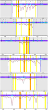 |
Fig. 2 Observed spectrum (black) of the bulge star B6-F1 (S/N = 54). The lines for abundance determination of Zr (three lines), La, Ce, and Eu (one line each) are marked out as the orange regions. The yellow regions are the manually placed continuum and the red spectrum is the synthetic one. The segments within which the synthetic spectrum is modelled are marked as the white wavelength regions between the blue vertical lines in each panel. The four horizontal lines above each spectrum indicate the lines’ sensitivity in the stellar parameters Teff, log g, [Fe/H] and ξmicro, respectively, where green is more sensitive than blue. |
3.2 Stellar parameters
The stellar parameters used are determined in Jönsson et al. (2017a,b) (where a more detailed description can be found) by fitting synthetic spectra for unsaturated and unblended Fe I and Fe II lines, Ca I lines, and log g sensitive Ca I line wings, whileTeff, log g, [Fe/H], ξmicro, and [Ca/Fe]were set as free parameters in SME. The Fe I line has NLTE corrections adopted from Lind et al. (2012). The reported uncertainties for these parameters in Jönsson et al. (2017a,b) for a typical disk star of S∕N ~ 100 are Teff ±50 K, log g ± 0.15 dex, [Fe/H] ± 0.05 dex, and ±0.1 km s−1 for ξmicro. For a typical bulge star, the S/N is significantly lower (median of 38), and hence the uncertainties greater; Teff ± 100 K, log g ± 0.30 dex, [Fe/H] ± 0.10 dex and ξmicro ± 0.2 km s−1. These values are later used in the uncertainties estimations; see Sect. 4.2.
3.3 Abundance determination
The atomic line data used for the abundance determination are collected from the Gaia-ESO line list version 6 (Heiter et al. 2015, and in prep.). From here we get wavelengths, excitation energies, and transition probabilities (as well as broadening parameters, when existing). The transition probabilities for the elements investigated here, Zr, La, Ce, and Eu, come from Biemont et al. (1981), Lawler et al. (2001a), Lawler et al. (2009), and Lawler et al. (2001b), respectively. All available lines for these elements in the given wavelength region (5800–6800 Å) were investigated individually in order to exclude lines that could not be modelled properly (due to blends, bad atomic data, or other systematics). As for Zr, where three separate lines were suitable for abundance determination, the lines were ultimately fitted simultaneously. Finally, the determined SME abundances were, in the post-process, re-normalised to the most up-to-date solar values provided by Grevesse et al. (2015). The final set of lines used for abundance determination is presented in Table 1. Apart from the atomic lines, we include the molecules C2 (Brooke et al. 2013) and CN (Sneden et al. 2014) in the synthesis.
For La and Eu, hyperfine splitting (hfs) had to be taken into account. By not taking hfs into account there is a risk of overestimating the measured abundance (Prochaska & McWilliam 2000; Thorsbro et al. 2018). Additionally, isotopic shift (IS) has to be considered for Zr, Ce, and Eu. The shift is caused by the isotopes having shifted energy levels, resulting in radiative transitions with shifted wavelengths. Isotopic shift is included by manually identifying the set of transitions for each isotope in the line list and scaling the log (gf) to the relative solar isotopic abundances; see Table 2.
3.4 Population separation
The classification of the stellar populations in the disk (thin/ thick) can be done in several ways, namely by kinematics, age, geometry, and chemistry. Even so, the separation of these two components is somewhat debated and the transition between them might be a gradient rather than a clear separation. The results by Hayden et al. (2015) show that the scale length of the thin disk extends further out than that of the thick disk. The thick disk has been shown to be enriched in α-elements compared to that of the thin disk, in addition to thick disk stars having higher total velocities but slower rotational velocities (Bensby et al. 2014).
In Lomaeva et al. (2019) the separation into the two populations is computed for our disk sample, using a combination of stellar metallicity, abundances ([Ti/Fe] as determined in Jönsson et al. 2017b) and kinematics. The radial velocities from Table A.2, propermotions from Gaia DR2 (Gaia Collaboration 2016, 2018) and distances from McMillan (2018) are used to calculate the total velocities4. In total, kinematic data were available for 268 stars in the disk sample. The clustering method Gaussian Mixture Model (GMM), obtained from the scikit-learn module for Python (Pedregosa et al. 2011), is used to cluster the disk data into the two components. We refer to Lomaeva et al. (2019) for more details.
Atomic lines used in the analysis.
Isotope information of the elements.
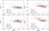 |
Fig. 3 Abundance ratio trends with metallicity, [X/Fe] against [Fe/H], for the thin- (blue) and thick-disk (yellow) stars as well as the bulge stars (red). Since it was not possible to determine all abundances in all spectra, the number of stars in each sample is included in the legend. Filled dark red circles indicate bulge stars with a S/N above 20, whereas the hollow red circles indicate a S/N equal to or less than 20. Some of the disk stars could not be classified as thick or thin disk stars; these are marked as grey dots. The typical uncertainty for the disk and the bulge sample, as described in Sect. 4.2, is marked in the lower right corner of every plot. |
4 Results
4.1 Abundances
Our derived abundance ratios, [X/Fe], for Zr, La, Ce, and Eu, are plotted against [Fe/H] in Fig. 3. The population separation is applied to the disk sample and the number of stars in each population for which we could determine the abundance in question is noted in every panel. The bulge sample is plotted on top of the disk trends, where for the bulge we differentiate between spectra of high and low S/N, with a separation of S/N = 20. The typical uncertainties are noted in the plots, and the estimation of these is described in Sect. 4.2.
4.2 Uncertainties
Systematic errors generally originate from incorrectly determined stellar parameters, model atmosphere assumptions, continuum placement, and atomic data. This makes these errors hard to estimate. To get a sense of the systematic uncertainties, one can compare to reference stars. In Jönsson et al. (2017a) they compare the determined stellar parameters to those of three overlapping Gaia benchmark stars determined in Jofré et al. (2015) and find that these are within the uncertainties of the Gaia benchmark parameters.
All spectra are analysed using the same line and continuum masks as well as the same atomic data, minimising possible random uncertainties. Therefore, the random uncertainties are to primarily be found in the (random) uncertainties of the stellar parameters. An approach to estimate the random uncertainties due to changes in the stellar parameters, is to analyse a typical spectrum several times using parameters that all vary within given distributions. The same method for estimating the uncertainties was used in Lomaeva et al. (2019).
Using the FIES spectrum of the standard star Arcturus5, uncertainties were added to its initial stellar parameters, meaning that the stellar parameters were changed simultaneously, for a set of 500 runs with modified stellar parameters. A Gaussian distribution is used to generate the uncertainties, using the reported stellar parameter uncertainties as standard deviation (see Sect. 3.2). In the uncertainty estimation of the bulge abundances, we have not degraded the FIES Arcturus spectrum (with a resolution of 67 000) to match that of the bulge spectra (R of 47 000), but separate tests have shown this slightly lower resolution to have a negligible effect on the determined abundance.
The abundance uncertainties coming from the uncertainties in the stellar parameters are then calculated as
![Mathematical equation: \begin{equation*}\sigma A_{\textrm{parameters}} = \sqrt{|\delta A_{T_{\textrm{eff}}}|^2 + |\delta A_{\log g}|^2 + |\delta A_{\textrm{[Fe/H]}}|^2 + |\delta A_{v_{\textrm{micro}}}|^2}, \end{equation*}](/articles/aa/full_html/2019/11/aa36343-19/aa36343-19-eq3.png) (1)
(1)
where, for non-symmetrical abundance changes, the mean value is used in the squared sums. The resulting uncertainties can be seen in Table 3.
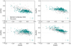 |
Fig. 4 Determined disk abundances in this work (teal) compared with the determined abundances from Battistini & Bensby (2016) (grey). The typical uncertainties for both data sets are indicated in the lower right corner of every plot, where the uncertainties are taken from Table 6 in Battistini & Bensby (2016). |
Estimated typical uncertainties for the disk and bulge sample using a generated set of stellar parameters for the giant star α-Boo.
5 Discussion
In this section we elaborate on the results. Firstly, we compare our separate abundance trends for the disks and bulge with previous literature studies in Sect. 5.1. Secondly, and this is the core of this investigation, in Sect. 5.2 we consider a more in-depth comparative analysis between our abundances for the bulge and disks populations, both determined in the same way. This is done to minimise the systematic uncertainties as much as possible. We then proceed in considering and discussing comparative abundance ratios such as [Eu/Mg], [Eu/La], and [second-peak s/first-peak s], also in Sect. 5.2 as well as Sect. 5.3.
To highlight features of the trend-plots, the running means of the samples are calculated and plotted (with a 1σ scatter). The number of data points in the running window is set to roughly 15% of the sample sizes (thin disk, thick disk, bulge). As a result, the running mean (and scatter) does not cover the whole trend range. For the bulge sample, only data points with S/N > 20 are includedin the running mean. Henceforth, the running mean-trend is the one referred to when describing [X/Fe] or [X/Y] ratios (except for Sect. 5.1.1).
5.1 Comparison with selected literature trends
5.1.1 Disk sample
In Fig. 4 we compare our determined disk abundances with those determined for dwarf stars in the disk by Battistini & Bensby (2016). In general, the trends are similar for all elements, as well as the scatter in the determined abundance. The abundances of [La, Ce, Eu/Fe] seem to be systematically higher than those of Battistini & Bensby (2016) whereas the [Zr/Fe]-abundances appear to be slightly lower. The typical abundance uncertainties for Battistini & Bensby (2016) are 0.12, 0.11, 0.12, and 0.08 dex for Zr, La, Ce, and Eu, respectively (their Table 6), which is somewhat higher than ours (see Table 3). The possible shifts in the abundances could be due to systematic differences in dwarf and giant stars or in differing atomic data such as using different lines in the abundance determination. Indeed, there is no overlap in the atomic lines used in these two data sets, except for the La line at 6390 Å, although Battistini & Bensby (2016) use three additional lines for the La abundance determination.
Zirconium is a first-peak s-process element whereas La and Ce are second-peak s-process elements. [Zr,La/Fe] have somewhat decreasing abundances with increasing metallicities, with a flattening of abundances for [Fe/H] above approximately − 0.4. The [Ce/Fe] trend is flatter than [Zr/Fe] and [La/Fe], explained by the higher s-process contribution in the Ce production (66, 76 and 84% s-process contribution for Zr, La and Ce, respectively Bisterzo et al. 2014).
The scatter for the [La/Fe] abundances is higher, ~0.5 dex, over themetallicity range [−0.2, 0], compared to the rest of the metallicity domain with ~0.3 dex. This indicates that AGB stars produce the bulk of their s-elements through the main s-process. The increase in scatter can most likely be explained by the mass range of AGB stars, which enables (1) stars to produce s-process elements at different metallicities (times) as well as (2) different amounts of production of the first-/second-peak s-process for AGB stars with different masses (see Sect. 5.3). The increasing abundances when [Fe/H] is below −0.5 for the s-process elements Zr and La point at a production by the r-process at early times (see [Eu/Fe]). In addition to Battistini & Bensby (2016), our results are comparable to those reported in Mishenina et al. (2013) (Zr, La, Ce, Eu) and Delgado Mena et al. (2017) (Zr, Ce, Eu), on dwarf stars in the local disk; see Fig. 5. The typical uncertainties from Mishenina et al. (2013) and Delgado Mena et al. (2017) are chosen from their estimates of low Teff stars; see their Tables 3 and 4, respectively.
For Eu, the trend decreases with increasing metallicity throughout our metallicity range, except for a plateau around [Fe/H] <−0.6. Europium has a reported r-process contribution of 94% (Bisterzo et al. 2014) and the observed trend indicates that the r-process has a continuous enrichment in the Galaxy, similar to that of the α-elements. Our Eu abundances compare well with those of Guiglion et al. (2018), including some subgiant and giant stars in their sample; see Fig. 5. We note that our measurements, and those of Battistini & Bensby (2016) and Guiglion et al. (2018), show, on average, slightly supersolar [Eu/Fe] abundances at solar metallicities, which is not seen in either Mishenina et al. (2013) or Delgado Mena et al. (2017). Of all the trends, ours is systematically high, not passing through the solar value at any metallicities.
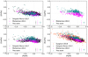 |
Fig. 5 Determined disk abundances in this work (teal) compared with selected literature trends: Mishenina et al. (2013) (pink), Delgado Mena et al. (2017) (black), and Guiglion et al. (2018) (orange). The typical uncertainties, when available, are indicated in the lower right corner of every plot, where the uncertainties from Mishenina et al. (2013) and Delgado Mena et al. (2017) (their Tables 3 and 4, respectively) are for a low Teff star. |
5.1.2 Bulge sample
In Fig. 6 we compare our bulge trend with those observed in Johnson et al. (2012), Van der Swaelmen et al. (2016), and Duong et al. (2019). Twenty-seven of our stars and their spectra overlap with those of Van der Swaelmen et al. (2016), and the same spectral lines are used for the abundance determination. Nonetheless, we observe different trends as well as measure Zr in these stars.
Zirconium
In general, our [Zr/Fe] trend with metallicity is flat, with an increase at lower metallicities [Fe/H] < −0.5. It should be noted that the running mean is rather poorly defined at the edges and the feature is based primarily on the two most metal-poor stars in Fig. 3. Our trend agrees well with that of Johnson et al. (2012) within our overlapping metallicity ranges, whereas Duong et al. (2019) has overall decreasing abundances with increasing metallicities. Above [Fe/H] ~ 0.1, our [Zr/Fe] is solar while Johnson et al. (2012) and Duong et al. (2019) have subsolar [Zr/Fe], ours pointing at a higher s-process contribution in the production of Zr.
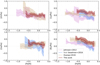 |
Fig. 6 Running mean for the bulge abundances determined in this work (red solid line) compared with the calculated running mean based on the abundances in Johnson et al. (2012) (pink solid line),Van der Swaelmen et al. (2016) (blue solid line), and Duong et al. (2019) (beige solid line), with a 1σ scatter (shaded regions, same colours as solid lines). |
Lanthanum
Johnson et al. (2012) reports a dip in [La/Fe] abundance around [Fe/H] ~−0.4 which is not observed in either of the other studies, or ours. Both Johnson et al. (2012) and Van der Swaelmen et al. (2016) produce decreasing [La/Fe] abundances with increasing metallicities, whilst both ours and that of Duong et al. (2019) exhibit only a very small decrease of [La/Fe] with increasing [Fe/H]. In general, our [La/Fe] abundances are higher than the other studies, which possibly could point at a higher s-process production in the bulge compared to previous work. However, we note that our bulge abundances, similarly to the disk abundances, are expected to suffer from a systematic offset in the determined [La/Fe] abundance ratios, preventing us from making a firm claim.
Cerium
Our [Ce/Fe] trend is flat throughout our metallicity range. Duong et al. (2019) also find a flat trend at solar scaled values, but with a slight step-wise increase at [Fe/H] ~−0.3, thereafter following our trend. Van der Swaelmen et al. (2016) find a different [Ce/Fe] trend with decreasing [Ce/Fe] values with increasing metallicities.
Europium
All the published [Eu/Fe] bulge trends and ours decrease with increasing metallicity, although with slightly different slopes and different offsets. The Johnson et al. (2012) study covers the lowest metallicities of all the samples. The trend of Duong et al. (2019) and ours trace each other closely with super-solar abundances at all metallicities. The Johnson et al. (2012) and Van der Swaelmen et al. (2016) trends follow each other well in their overlapping metallicity region, with subsolar abundances above solar metallicities. There is an observable “knee” in the trend around [Fe/H] ~ − 0.4, seen in all four studies mentioned above. Similarly to [La/Fe], our [Eu/Fe] abundances are higher than those in previous studies, although due to the possible systematic offsets we cannot draw any firm conclusions from this. However, since the main purpose of this work is to make a differential analysis between the disk and bulge abundances in this work, the possible systematic offset in our analysis is of less importance.
5.2 Disk and bulge comparison of the current study
In this section we compare our abundance-ratio trends, that is [X/Fe], for the bulge, the thin disk, and the thick disk as a function of the metallicity for the s-process elements Zr, La, and Ce, and the r-process element Eu. In Fig. 7 we directly compare thebulge population trends with those of the thin and the thick disk populations, determined in the same way in the present study.
The bulge and the disks have very similarly shaped s-process element trends (Zr, La, Ce). The bulge trend of [La/Fe] is slightly higher overall, especially at subsolar metallicities where [La/Fe] is ~ 0.1 dex higher than for the disk. We note that this is the opposite to findings in Duong et al. (2019). The metallicities of the bulge sample extend to slightly higher values, pointing at a higher star formation rate of the bulge. Additionally, Matteucci et al. (2019) shows that implementing a Salpeter like initial mass function (IMF), which favours massive stars compared to typical IMFs for the disk, better reproduce bulge abundances.
For [Eu/Fe], the thick disk is enhanced as compared with the thin disk, reminding us of an α-element. The decreasing trend for metallicities larger than [Fe/H] ≳−0.4 is a result of iron production by SN Ia after a time delay of roughly 100 Myr-1 Gyr (Matteucci & Brocato 1990; Ballero et al. 2007). The bulge traces the thick disk in the [Eu/Fe] abundance, suggesting the bulge has a similar star formation rate as that of the thick disk. A plateau, or a knee, can be seen around metallicities of approximately − 0.4 for both the thick disk and the bulge. A knee at higher metallicities than in the solar vicinity was already predicted for the bulge by Matteucci & Brocato (1990) and in general for systems with higher star formation rates than in the solar vicinity.
In Fig. 8 we compare Eu with the well-determined α-element magnesium (from Jönsson et al. 2017b), by plotting [Eu/Mg], for the same stars. The resulting, mostly flat trend of all populations is already expected from the [Eu/Fe] trend, pointing at Eu having a contribution from progenitors of similar timescales to that of progenitors producing Mg (i.e. SNe II). It has indeed been shown by Travaglio et al. (1999) that SNe II progenitors with masses of 8–10 M⊙ best reproduce the r-process enrichment in the Galaxy, and Cescutti et al. (2006) showed that to reproduce the ratio of typical s-process elements, such as [Ba/Fe], at low metallicities, an r-process production of these elements in stars with masses ranging from 8 to 30 M⊙ should be assumed. Nonetheless, the origin of r-elements is, as mentioned earlier, still debated (see e.g. Sneden et al. 2000; Thielemann et al. 2011; Côté et al. 2019; Siegel et al. 2019; Kajino et al. 2019).
A way to disentangle the s- and r-process contribution throughout the evolution of the Galaxy is to compare an s-process-dominated element with an r-process-dominated one. We thus compare La, with an s-process contribution of 76%, to that of Eu with an r-process contribution of 94% (Bisterzo et al. 2014), plotted as [La/Eu] in Fig. 9. A pure r-process line is added, using the values from Bisterzo et al. (2014). The value of the pure r-process line is calculated by subtracting the predicted s-process abundance from the solar system total values, that is, by treating the r-process as a residual (Bisterzo et al. 2014).
The trends in Fig. 9 show that the r-process increasingly dominates the production of neutron-capture elements with decreasing metallicity, reaching [La/Eu] = −0.25 for the bulge and [La/Eu] = −0.4 for the thick disk at [Fe/H] ~−0.5. With regard to the large scatter at supersolar metallicities, we refrain from making any further interpretations of the bulge abundances at these metallicities. At around [Fe/H] ~−0.6 the [La/Eu] thick disk trend levels off or even increases with lower metallicities. Whether this is significant or not is yet to be understood and observations of more stars in this metallicity range are needed. The generally higher [La/Eu] abundances of the bulge compared with those of the thick disk point at the bulge having either less r-process production (in turn, possibly a different amount of SNe II), or a higher s-process contribution (as seen previously in the [La/Fe]-trend) than that of the thick disk.
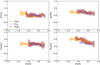 |
Fig. 7 Running mean for the bulge (red solid line) compared with the running mean of the thick disk (yellow solid line) and thin disk (blue solid line), with a 1σ scatter (shaded regions, same colours as solid lines). |
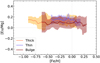 |
Fig. 8 [Eu/Mg] abundances against [Fe/H] as running mean with a 1σ scatter for the thin disk (blue), thick disk (yellow), and bulge (red). |
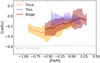 |
Fig. 9 [La/Eu] abundances against [Fe/H] as running mean with a 1σ scatter for the thin disk (blue), thick disk (yellow), and bulge (red). A pure r-process line is plotted, calculated using the values presented in Bisterzo et al. (2014). |
5.3 First- and second-peak s-process elements
In Fig. 10, the running mean of the ratio of the second-peak s-process elements (a mean of La and Ce) and the first-peak s-process element Zr are plotted against metallicity. The trend, elaborated on in the last paragraph of this section,can be explained by considering the stellar yields from Karakas & Lugaro (2016), where low-mass AGB stars have a higher relative production of second-peak elements compared to the production of first-peak elements.
The neutrons in the s-process come from two neutron sources: the  O- and the
  Mg-reactions. The 13C source has a lower neutron density of roughly 107 neutrons cm−3, whereas the neutron density for the 22Ne source is around 1015 neutrons cm−3. However, due to the longer timescales of the 13C reaction (~103 yr compared to~10 yr), the time integrated neutron flux for this neutron source is much higher than for the 22Ne source. Due to this, the 13C reac- tion builds up the heavier s-process elements, such as the second- (and third-)peak elements, whilst the 22Ne reaction is limited to producing the first-peak s-process elements (Karakas & Lattanzio 2014).
Furthermore, Bisterzo et al. (2017) elaborate on the importance of the size of the 13C-pocket in the s-process production. The 22Ne reaction takes place only in initially more massive (AGB) stars of >4 M⊙, due to the higher temperatures of these stars (Karakas & Lattanzio 2014). This shrinks the 13C-pocket, resulting in a smaller quantity of s-elements being expected, especially the heavier ones. In short, heavier AGB stars produce relatively fewer second-peak elements compared to low-mass AGB stars, and the latter have a longer time delay.
Another aspect to keep in mind is that at lower metallicities, the ratio of the number of neutrons to the number of available 56Fe-seeds is higher, compared to higher metallicities, which enables the build-up of second-peak elements (Busso et al. 1999).
In Fig. 10 we first see an increasing trend in the thick disk for increasing metallicities, which turns over for solar metallicities and higher. Below solar metallicities (and above [Fe/H] ~−0.5), all trends show an enrichment of second-peak as compared to first-peak elements. This is therefore explained by the low-mass AGB stars which have not yet enriched the interstellar medium (ISM) at the time of the formation of the older thick disk stars, resulting in relatively low [(La+Ce)/Zr] abundances at early times.
At solar metallicities, the disk populations does not show any clear differences. As for the bulge, it follows the trend of the thick disk more closely than that of the thin disk at subsolar metallicities. At supersolar metallicities, the first-peak elements seem to increase in the bulge, possibly explained by a contribution of metal-rich AGB stars, producing a higher amount of first-peak elements (Karakas & Lugaro 2016).
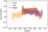 |
Fig. 10 Abundance ratio of the second-peak s-process elements (La, Ce) and the first-peak s-process element (Zr) against [Fe/H] as running mean with a 1σ scatter for the thin disk (blue), thick disk (yellow), and bulge (red). |
6 Conclusions
In this work we determined abundances of the neutron-capture elements Zr, La, Ce, and Eu in 45 bulge giants and 291 local disk giants. The determination has been done using high-resolution spectra obtained with FLAMES/UVES (bulge sample) or either FIES or PolarBase (disk sample) and the analysis code SME.
All spectra are evaluated over the wavelength region 5800–6800 Å and the careful, manual definition of the continuum surrounding the spectral lines of interest in the spectra has been crucial in order to get high-precision abundances. Hyperfine splitting (in the cases of La, Eu) has been taken into account, as well as isotopic shifts by manually scaling the log (gf)-values of the identified transitions in the line list (for the isotopes of Zr, Ce, Eu).
The stellar mass and metallicity are factors that contribute to, and affect, the s- and r-process production. Due to this, the enrichment of the ISM and the abundance of neutron-capture elements vary with time in the Galaxy, making them suitable probes for Galactic chemical evolution.
Our [Zr, La, Ce/Fe] bulge trends are in general flatter than those reported by previous studies, many of which are decreasing with higher metallicities. Such decreasing trends would suggest a higher r-process contribution to these elements in the bulge, while our flatter trends that have the same general shapes as our thick disk trends suggest more similar r/s-proportions in the creation of the neutron capture elements in the bulge and disks. The [La/Fe] bulge trend is ~ 0.1 dex higher compared with the disk, possibly indicating a higher s-process contribution in the bulge, compared with that of the disk.
For [Eu/Fe], we see a decreasing trend with increasing metallicities for both the disk and the bulge, with a plateau at around [Fe/H] ~ −0.4. This is very similar to the typical α-element trend, and plotting [Eu/Mg] confirms this, suggesting that the r-process has a similar production rate as that of Mg (coming from SNe II).
For [La/Eu] we find that towards low metallicities, the abundances lay closer to the pure r-process line (reaching [La/Eu] − 0.4 (disk) and − 0.25 (bulge) at [Fe/H] ~−0.5), indicating that the r-process was the dominating neutron-capture process at early times, both in the disk and the bulge. The results also point at either (a) a different amount of massive stars or (b) different contribution of the s-process in the local thick disk and the bulge, where the [La/Eu] abundances seem to be systematically higher in the bulgethan in the thick disk. Since we compare abundances determined with the same method, and for stars at the same evolutionary stage, the difference between the disk and the bulge in [La/Fe] could likely be real.
When plotting the ratio of the second- and first-peak s-process elements, [(La+Ce)/Zr], against metallicity we see that the bulge and the thick disk trends follow each other closely. We also show that, according to theoretical predictions by Karakas & Lattanzio (2014), low-mass AGB stars are needed to explain the enhancement of second-peak s-process abundances compared to first-peak s-process abundances.
To conclude, in general, our findings for Zr, Ce and Eu suggest that the bulge experiences a similar chemical evolution to that of the local thick disk, with a similar star formation rate. On the other hand, our La trends for the bulge and the thick disk are offset by about 0.1: systematic effects could not be identified in our homogeneous analysis of the bulge and disk samples and further investigation is still required. Our results for the s-process elements differ substantially from previous studies: here we find flatter trends. More bulge data would be needed to decrease thescatter and put further constraints on bulge abundances. Additionally, it would be useful to adopt the abundances in Galactic Chemical Evolution models to put further constraints on the evolution of the Galaxy and its components.
Acknowledgements
We would like to thank the referee, Mathieu Van der Swaelmen, for very insightful comments and suggestions which helped to improve this paper in many ways. This research has been partly supported by the Lars Hierta Memorial Foundation, and the Royal Physiographic Society in Lund through Stiftelsen Walter Gyllenbergs fond and Märta och Erik Holmbergs donation. H.J. acknowledges support from the Crafoord Foundation, Stiftelsen Olle Engkvist Byggmästare, and Ruth och Nils-Erik Stenbäcks stiftelse. This work has made use of data from the European Space Agency (ESA) mission Gaia (https://www.cosmos.esa.int/gaia), processed by the Gaia Data Processing and Analysis Consortium (DPAC, https://www.cosmos.esa.int/web/gaia/dpac/consortium). Funding for the DPAC has been provided by national institutions, in particular the institutions participating in the Gaia Multilateral Agreement. This publication made use of the SIMBAD database, operated at CDS, Strasbourg, France; NASA’s Astrophysics Data System; and the VALD database, operated at Uppsala University, the Institute of Astronomy RAS in Moscow, and the University of Vienna.
Appendix A: Additional tables
Basic data for the observed bulge giants.
Basic data for the observed solar neighbourhood giants.
Stellar parameters and determined abundances for observed bulge giants.
Stellar parameters and determined abundances for observed solar neighbourhood giants.
References
- Abbott, B. P., Abbott, R., Abbott, T. D., et al. 2017, Phys. Rev. Lett., 119, 161101 [NASA ADS] [CrossRef] [PubMed] [Google Scholar]
- Bailer-Jones, C. A. L., Rybizki, J., Fouesneau, M., Mantelet, G., & Andrae, R. 2018, AJ, 156, 58 [NASA ADS] [CrossRef] [Google Scholar]
- Ballero, S. K., Matteucci, F., Origlia, L., & Rich, R. M. 2007, A&A, 467, 123 [Google Scholar]
- Barbuy, B., Chiappini, C., & Gerhard, O. 2018, ARA&A, 56, 223 [NASA ADS] [CrossRef] [Google Scholar]
- Battistini, C., & Bensby, T. 2016, A&A, 586, A49 [NASA ADS] [CrossRef] [EDP Sciences] [Google Scholar]
- Bensby, T., Feltzing, S., & Oey, M. S. 2014, A&A, 562, A71 [NASA ADS] [CrossRef] [EDP Sciences] [Google Scholar]
- Biemont, E., Grevesse, N., Hannaford, P., & Lowe, R. M. 1981, ApJ, 248, 867 [NASA ADS] [CrossRef] [Google Scholar]
- Bisterzo, S., Travaglio, C., Gallino, R., Wiescher, M., & Käppeler, F. 2014, ApJ, 787, 10 [NASA ADS] [CrossRef] [Google Scholar]
- Bisterzo, S., Travaglio, C., Wiescher, M., Käppeler, F., & Gallino, R. 2017, ApJ, 835, 97 [NASA ADS] [CrossRef] [Google Scholar]
- Brooke, J. S. A., Bernath, P. F., Schmidt, T. W., & Bacskay, G. B. 2013, J. Quant. Spectr. Rad. Transf., 124, 11 [NASA ADS] [CrossRef] [Google Scholar]
- Buder, S., Asplund, M., Duong, L., et al. 2018, MNRAS, 478, 4513 [NASA ADS] [CrossRef] [Google Scholar]
- Burbidge, E. M., Burbidge, G. R., Fowler, W. A., & Hoyle, F. 1957, Rev. Mod. Phys., 29, 547 [NASA ADS] [CrossRef] [Google Scholar]
- Busso, M., Gallino, R., & Wasserburg, G. J. 1999, ARA&A, 37, 239 [NASA ADS] [CrossRef] [Google Scholar]
- Cardelli, J. A., Clayton, G. C., & Mathis, J. S. 1989, ApJ, 345, 245 [NASA ADS] [CrossRef] [Google Scholar]
- Cescutti, G., François, P., Matteucci, F., Cayrel, R., & Spite, M. 2006, A&A, 448, 557 [NASA ADS] [CrossRef] [EDP Sciences] [Google Scholar]
- Chang, T. L., Qian, Q.-Y., Zhao, M.-T., & Wang, J. 1994, Int. J. Mass Spectrom. Ion Process., 139, 95 [NASA ADS] [CrossRef] [Google Scholar]
- Chang, T.-L., Qian, Q.-Y., Zhao, M.-T., Wang, J., & Lang, Q.-Y. 1995, Int. J. Mass Spectrom. Ion Process., 142, 125 [NASA ADS] [CrossRef] [Google Scholar]
- Côté, B., Eichler, M., Arcones, A., et al. 2019, ApJ, 875, 106 [NASA ADS] [CrossRef] [Google Scholar]
- Couch, R. G., Schmiedekamp, A. B., & Arnett, W. D. 1974, ApJ, 190, 95 [NASA ADS] [CrossRef] [Google Scholar]
- Cristallo, S., Abia, C., Straniero, O., & Piersanti, L. 2015, ApJ, 801, 53 [NASA ADS] [CrossRef] [Google Scholar]
- de Laeter, J. R., & Bukilic, N. 2005, Int. J. Mass Spectrom., 244, 91 [NASA ADS] [CrossRef] [Google Scholar]
- Delgado Mena, E., Tsantaki, M., Adibekyan, V. Z., et al. 2017, A&A, 606, A94 [NASA ADS] [CrossRef] [EDP Sciences] [Google Scholar]
- Duong, L., Asplund, M., Nataf, D. M., Freeman, K. C., & Ness, M. 2019, MNRAS, 486, 5349 [NASA ADS] [CrossRef] [Google Scholar]
- Gaia Collaboration (Prusti, T., et al.) 2016, A&A, 595, A1 [NASA ADS] [CrossRef] [EDP Sciences] [Google Scholar]
- Gaia Collaboration (Brown, A. G. A., et al.) 2018, A&A, 616, A1 [NASA ADS] [CrossRef] [EDP Sciences] [Google Scholar]
- Gonzalez, O. A., Rejkuba, M., Zoccali, M., et al. 2011, A&A, 530, A54 [NASA ADS] [CrossRef] [EDP Sciences] [Google Scholar]
- Gonzalez, O. A., Rejkuba, M., Zoccali, M., et al. 2012, A&A, 543, A13 [NASA ADS] [CrossRef] [EDP Sciences] [Google Scholar]
- Gonzalez, O. A., Zoccali, M., Vasquez, S., et al. 2015, A&A, 584, A46 [NASA ADS] [CrossRef] [EDP Sciences] [Google Scholar]
- Grevesse, N., Asplund, M., & Sauval, A. J. 2007, Space Sci. Rev., 130, 105 [Google Scholar]
- Grevesse, N., Scott, P., Asplund, M., & Sauval, A. J. 2015, A&A, 573, A27 [NASA ADS] [CrossRef] [EDP Sciences] [Google Scholar]
- Gruyters, P., Lind, K., Richard, O., et al. 2016, A&A, 589, A61 [NASA ADS] [CrossRef] [EDP Sciences] [Google Scholar]
- Guiglion, G., de Laverny, P., Recio-Blanco, A., & Prantzos, N. 2018, A&A, 619, A143 [NASA ADS] [CrossRef] [EDP Sciences] [Google Scholar]
- Gustafsson, B., Edvardsson, B., Eriksson, K., et al. 2008, A&A, 486, 951 [NASA ADS] [CrossRef] [EDP Sciences] [Google Scholar]
- Hayden, M. R., Bovy, J., Holtzman, J. A., et al. 2015, ApJ, 808, 132 [NASA ADS] [CrossRef] [Google Scholar]
- Heiter, U., Lind, K., Asplund, M., et al. 2015, Phys. Scr, 90, 054010 [CrossRef] [Google Scholar]
- Herwig, F. 2005, ARA&A, 43, 435 [NASA ADS] [CrossRef] [Google Scholar]
- Hinkle, K., Wallace, L., Harmer, D., Ayres, T., & Valenti, J. 2000, IAU Joint Discuss., 24, 26 [Google Scholar]
- Immeli, A., Samland, M., Gerhard, O., & Westera, P. 2004, A&A, 413, 547 [NASA ADS] [CrossRef] [EDP Sciences] [Google Scholar]
- Jofré, P., Heiter, U., Soubiran, C., et al. 2015, A&A, 582, A81 [NASA ADS] [CrossRef] [EDP Sciences] [Google Scholar]
- Johnson,C. I., Rich, R. M., Kobayashi, C., & Fulbright, J. P. 2012, ApJ, 749, 175 [NASA ADS] [CrossRef] [Google Scholar]
- Jönsson, H., Ryde, N., Nordlander, T., et al. 2017a, A&A, 598, A100 [NASA ADS] [CrossRef] [EDP Sciences] [Google Scholar]
- Jönsson, H., Ryde, N., Schultheis, M., & Zoccali, M. 2017b, A&A, 600, C2 [NASA ADS] [CrossRef] [EDP Sciences] [Google Scholar]
- Kajino, T., Aoki, W., Balantekin, A. B., et al. 2019, Prog. Part. Nucl. Phys., 107, 109 [NASA ADS] [CrossRef] [Google Scholar]
- Karakas, A. I., & Lattanzio, J. C. 2014, PASA, 31, e030 [NASA ADS] [CrossRef] [Google Scholar]
- Karakas, A. I., & Lugaro, M. 2016, ApJ, 825, 26 [NASA ADS] [CrossRef] [Google Scholar]
- Korn, A. J., Grundahl, F., Richard, O., et al. 2007, ApJ, 671, 402 [NASA ADS] [CrossRef] [Google Scholar]
- Kratz, K.-L., Farouqi, K., Pfeiffer, B., et al. 2007, ApJ, 662, 39 [NASA ADS] [CrossRef] [MathSciNet] [Google Scholar]
- Lawler, J. E., Bonvallet, G., & Sneden, C. 2001a, ApJ, 556, 452 [NASA ADS] [CrossRef] [Google Scholar]
- Lawler, J. E., Wickliffe, M. E., den Hartog, E. A., & Sneden, C. 2001b, ApJ, 563, 1075 [CrossRef] [Google Scholar]
- Lawler, J. E., Sneden, C., Cowan, J. J., & Ivans, I. I., & Den Hartog E. A. 2009, ApJS, 182, 51 [NASA ADS] [CrossRef] [Google Scholar]
- Lecureur, A., Hill, V., Zoccali, M., et al. 2007, A&A, 465, 799 [NASA ADS] [CrossRef] [EDP Sciences] [Google Scholar]
- Lind, K., Korn, A. J., Barklem, P. S., & Grundahl, F. 2008, A&A, 490, 777 [NASA ADS] [CrossRef] [EDP Sciences] [Google Scholar]
- Lind, K., Bergemann, M., & Asplund, M. 2012, MNRAS, 427, 50 [NASA ADS] [CrossRef] [Google Scholar]
- Liu, F., Asplund, M., Yong, D., et al. 2019, A&A, 627, A117 [NASA ADS] [CrossRef] [EDP Sciences] [Google Scholar]
- Lomaeva, M., Jönsson, H., Ryde, N., Schultheis, M., & Thorsbro, B. 2019, A&A, 625, A141 [NASA ADS] [CrossRef] [EDP Sciences] [Google Scholar]
- Marquardt, D. W. 1963, J. Soc. Ind. Appl. Math., 11, 431 [Google Scholar]
- Mashonkina, L., & Gehren, T. 2000, A&A, 364, 249 [NASA ADS] [Google Scholar]
- Matteucci, F., & Brocato, E. 1990, ApJ, 365, 539 [NASA ADS] [CrossRef] [Google Scholar]
- Matteucci, F., Grisoni, V., Spitoni, E., et al. 2019, MNRAS, 487, 5363 [NASA ADS] [CrossRef] [Google Scholar]
- McMillan, P. J. 2018, Res. Notes AAS, 2, 51 [Google Scholar]
- McWilliam, A. 2016, PASA, 33, e040 [NASA ADS] [CrossRef] [Google Scholar]
- Meléndez, J., Asplund, M., Alves-Brito, A., et al. 2008, A&A, 484, L21 [NASA ADS] [CrossRef] [EDP Sciences] [MathSciNet] [Google Scholar]
- Mishenina, T. V., Pignatari, M., Korotin, S. A., et al. 2013, A&A, 552, A128 [NASA ADS] [CrossRef] [EDP Sciences] [Google Scholar]
- Nomura, M., Kogure, K., & Okamoto, M. 1983, Int. J. Mass Spectrom. Ion Process., 50, 219 [NASA ADS] [CrossRef] [Google Scholar]
- Nordlander, T., Korn, A. J., Richard, O., & Lind, K. 2012, ApJ, 753, 48 [NASA ADS] [CrossRef] [Google Scholar]
- Pedregosa, F., Varoquaux, G., Gramfort, A., et al. 2011, J. Mach. Learn. Res., 12, 2825 [Google Scholar]
- Petit, P., Louge, T., Théado, S., et al. 2014, PASP, 126, 469 [NASA ADS] [CrossRef] [Google Scholar]
- Piskunov, N., & Valenti, J. A. 2017, A&A, 597, A16 [NASA ADS] [CrossRef] [EDP Sciences] [Google Scholar]
- Portail, M., Gerhard, O., Wegg, C., & Ness, M. 2017, MNRAS, 465, 1621 [NASA ADS] [CrossRef] [Google Scholar]
- Prochaska, J. X., & McWilliam, A. 2000, ApJ, 537, L57 [NASA ADS] [CrossRef] [Google Scholar]
- Shen, J., & Li, Z.-Y. 2016, in Galactic Bulges, eds. E. Laurikainen, R. Peletier, & D. Gadotti (Berlin: Springer), 418, 233 [NASA ADS] [CrossRef] [Google Scholar]
- Siegel, D. M., Barnes, J., & Metzger, B. D. 2019, Nature, 569, 241 [NASA ADS] [CrossRef] [Google Scholar]
- Sneden, C., Cowan, J. J., Ivans, I. I., et al. 2000, ApJ, 533, L139 [NASA ADS] [CrossRef] [PubMed] [Google Scholar]
- Sneden, C., Lucatello, S., Ram, R. S., Brooke, J. S. A., & Bernath, P. 2014, ApJS, 214, 26 [Google Scholar]
- Souto, D., Allende Prieto, C., Cunha, K., et al. 2019, ApJ, 874, 97 [NASA ADS] [CrossRef] [Google Scholar]
- Telting, J. H., Avila, G., Buchhave, L., et al. 2014, Astron. Nachr., 335, 41 [NASA ADS] [CrossRef] [Google Scholar]
- Thielemann, F.-K., Arcones, A., Käppeli, R., et al. 2011, Prog. Part. Nucl. Phys., 66, 346 [NASA ADS] [CrossRef] [Google Scholar]
- Thielemann, F. K., Eichler, M., Panov, I. V., & Wehmeyer, B. 2017, Ann. Rev. Nucl. Part. Sci., 67, 253 [NASA ADS] [CrossRef] [Google Scholar]
- Thielemann, F.-K., Isern, J., Perego, A., & von Ballmoos, P. 2018, Space Sci. Rev., 214, 62 [NASA ADS] [CrossRef] [Google Scholar]
- Thorsbro, B., Ryde, N., Schultheis, M., et al. 2018, ApJ, 866, 52 [NASA ADS] [CrossRef] [Google Scholar]
- Thygesen, A. O., Frandsen, S., Bruntt, H., et al. 2012, A&A, 543, A160 [NASA ADS] [CrossRef] [EDP Sciences] [Google Scholar]
- Travaglio, C., Galli, D., Gallino, R., et al. 1999, ApJ, 521, 691 [NASA ADS] [CrossRef] [Google Scholar]
- Travaglio, C., Gallino, R., Arnone, E., et al. 2004, ApJ, 601, 864 [NASA ADS] [CrossRef] [Google Scholar]
- Valenti, J. A.,& Piskunov, N. 1996, A&AS, 118, 595 [NASA ADS] [CrossRef] [EDP Sciences] [Google Scholar]
- Van der Swaelmen, M., Barbuy, B., Hill, V., et al. 2016, A&A, 586, A1 [NASA ADS] [CrossRef] [EDP Sciences] [Google Scholar]
- Velichko, A. B., Mashonkina, L. I., & Nilsson, H. 2010, Astron. Lett., 36, 664 [NASA ADS] [CrossRef] [Google Scholar]
- Wegg, C., Gerhard, O., & Portail, M. 2015, MNRAS, 450, 4050 [NASA ADS] [CrossRef] [Google Scholar]
- Weiland, J. L., Arendt, R. G., Berriman, G. B., et al. 1994, ApJ, 425, L81 [NASA ADS] [CrossRef] [Google Scholar]
- Zasowski, G., Schultheis, M., Hasselquist, S., et al. 2019, ApJ, 870, 138 [NASA ADS] [CrossRef] [Google Scholar]
Duong et al. (2019), to as large an extent as possible, use the same atomic data and analysis method in their work as their comparison sample, GALAH (Buder et al. 2018), to minimise systematic offsets.
The naming of the fields follows the convention seen in Lecureur et al. (2007).
Available at marcs.astro.uu.se
 .
.
The giant star Arcturus (also known as α-Boo or HIP69673) has been analysed extensively due to its brightness, being the fourth brightest in the night sky, and is suitable as a reference of a typical giant star.
All Tables
Estimated typical uncertainties for the disk and bulge sample using a generated set of stellar parameters for the giant star α-Boo.
Stellar parameters and determined abundances for observed solar neighbourhood giants.
All Figures
|
Fig. 1 Map of the Galactic bulge showing the five analysed fields (SW, B3, BW, B6, and BL). The bulge samples from Johnson et al. (2012), Van der Swaelmen et al. (2016), and Duong et al. (2019) are also marked in the figure. The dust extinction towards the bulge is taken from Gonzalez et al. (2011, 2012) and scaled to optical extinction (Cardelli et al. 1989). The scale saturates at AV = 2, which is the upper limit in the figure. The COBE/DIRBE contours of the Galactic bulge, in black, are from Weiland et al. (1994). |
| In the text | |
|
Fig. 2 Observed spectrum (black) of the bulge star B6-F1 (S/N = 54). The lines for abundance determination of Zr (three lines), La, Ce, and Eu (one line each) are marked out as the orange regions. The yellow regions are the manually placed continuum and the red spectrum is the synthetic one. The segments within which the synthetic spectrum is modelled are marked as the white wavelength regions between the blue vertical lines in each panel. The four horizontal lines above each spectrum indicate the lines’ sensitivity in the stellar parameters Teff, log g, [Fe/H] and ξmicro, respectively, where green is more sensitive than blue. |
| In the text | |
|
Fig. 3 Abundance ratio trends with metallicity, [X/Fe] against [Fe/H], for the thin- (blue) and thick-disk (yellow) stars as well as the bulge stars (red). Since it was not possible to determine all abundances in all spectra, the number of stars in each sample is included in the legend. Filled dark red circles indicate bulge stars with a S/N above 20, whereas the hollow red circles indicate a S/N equal to or less than 20. Some of the disk stars could not be classified as thick or thin disk stars; these are marked as grey dots. The typical uncertainty for the disk and the bulge sample, as described in Sect. 4.2, is marked in the lower right corner of every plot. |
| In the text | |
|
Fig. 4 Determined disk abundances in this work (teal) compared with the determined abundances from Battistini & Bensby (2016) (grey). The typical uncertainties for both data sets are indicated in the lower right corner of every plot, where the uncertainties are taken from Table 6 in Battistini & Bensby (2016). |
| In the text | |
|
Fig. 5 Determined disk abundances in this work (teal) compared with selected literature trends: Mishenina et al. (2013) (pink), Delgado Mena et al. (2017) (black), and Guiglion et al. (2018) (orange). The typical uncertainties, when available, are indicated in the lower right corner of every plot, where the uncertainties from Mishenina et al. (2013) and Delgado Mena et al. (2017) (their Tables 3 and 4, respectively) are for a low Teff star. |
| In the text | |
|
Fig. 6 Running mean for the bulge abundances determined in this work (red solid line) compared with the calculated running mean based on the abundances in Johnson et al. (2012) (pink solid line),Van der Swaelmen et al. (2016) (blue solid line), and Duong et al. (2019) (beige solid line), with a 1σ scatter (shaded regions, same colours as solid lines). |
| In the text | |
|
Fig. 7 Running mean for the bulge (red solid line) compared with the running mean of the thick disk (yellow solid line) and thin disk (blue solid line), with a 1σ scatter (shaded regions, same colours as solid lines). |
| In the text | |
|
Fig. 8 [Eu/Mg] abundances against [Fe/H] as running mean with a 1σ scatter for the thin disk (blue), thick disk (yellow), and bulge (red). |
| In the text | |
|
Fig. 9 [La/Eu] abundances against [Fe/H] as running mean with a 1σ scatter for the thin disk (blue), thick disk (yellow), and bulge (red). A pure r-process line is plotted, calculated using the values presented in Bisterzo et al. (2014). |
| In the text | |
|
Fig. 10 Abundance ratio of the second-peak s-process elements (La, Ce) and the first-peak s-process element (Zr) against [Fe/H] as running mean with a 1σ scatter for the thin disk (blue), thick disk (yellow), and bulge (red). |
| In the text | |
Current usage metrics show cumulative count of Article Views (full-text article views including HTML views, PDF and ePub downloads, according to the available data) and Abstracts Views on Vision4Press platform.
Data correspond to usage on the plateform after 2015. The current usage metrics is available 48-96 hours after online publication and is updated daily on week days.
Initial download of the metrics may take a while.