| Issue |
A&A
Volume 631, November 2019
|
|
|---|---|---|
| Article Number | A78 | |
| Number of page(s) | 14 | |
| Section | Extragalactic astronomy | |
| DOI | https://doi.org/10.1051/0004-6361/201834530 | |
| Published online | 23 October 2019 | |
A spectral stacking analysis to search for faint outflow signatures in z ∼ 6 quasars⋆
Department of Space, Earth and Environment, Chalmers University of Technology, Onsala Space Observatory, 439 92 Onsala, Sweden
e-mail: This email address is being protected from spambots. You need JavaScript enabled to view it.
Received:
29
October
2018
Accepted:
29
August
2019
Abstract
Aims. Outflows in quasars during the early epochs of galaxy evolution are an important part of the feedback mechanisms that potentially affect the evolution of the host galaxy. However, systematic millimetre (mm) observations of outflows are only now becoming possible with the advent of sensitive mm telescopes. In this study we used spectral stacking methods to search for a faint high-velocity outflow signal in a sample of [C II] detected, z ∼ 6 quasars.
Methods. We searched for broad emission line signatures from high-velocity outflows for a sample of 26 z ∼ 6 quasars observed with the Atacama Large Millimeter Array (ALMA), with a detection of the [C II] line. The observed emission lines of the sources are dominated by the host galaxy, and outflow emission is not detected for the individual sources. We used a spectral line stacking analysis developed for interferometric data to search for outflow emission. We stacked both extracted spectra and the full spectral cubes. We also investigated the possibility that only a sub-set of our sample contributes to the stacked outflow emission.
Results. We find only a tentative detection of a broad emission line component in the stacked spectra. When taking a region of about 2″ around the central position of the stacked cubes, the stacked line shows an excess emission due to a broad component of 1.1–1.5σ, but the significance drops to 0.4–0.7σ when stacking the extracted spectra from a smaller region. The broad component can be characterised by a line width of full width at half-maximum FWHM > 700 km s−1. Furthermore, we find a sub-sample of 12 sources, the stack of which maximises the broad component emission. The stack of this sub-sample shows an excess emission due to a broad component of 1.2–2.5σ. The stacked line of these sources has a broad component of FWHM > 775 km s−1.
Conclusions. We find evidence suggesting the presence of outflows in a sub-sample of 12 out of 26 sources, which demonstrates the importance of spectral stacking techniques in tracing faint signal in galaxy samples. However, deeper ALMA observations are necessary to confirm the presence of a broad component in the individual spectra.
Key words: galaxies: high-redshift / quasars: general / galaxies: evolution / submillimeter: galaxies
All reduced data cubes and all stacked cubes are only available at the CDS via anonymous ftp to cdsarc.u-strasbg.fr (130.79.128.5) or via http://cdsarc.u-strasbg.fr/viz-bin/cat/J/A+A/631/A78
© ESO 2019
1. Introduction
Our understanding of redshift z ≳ 6 galaxies and super-massive black holes (SMBHs) has increased significantly, and still continues to do so. More and more quasars are detected at high redshifts, with their numbers now in the hundreds at redshifts z > 5.5 (e.g. Bañados et al. 2016; Jiang et al. 2016). These quasars are known to have SMBH masses of > 109 M⊙ (e.g. Fan et al. 2006; Kurk et al. 2007; De Rosa et al. 2011). Their hosts tend to be massive galaxies with stellar masses of 1010 − 1011 M⊙. Star formation rates (SFRs) in z ∼ 6 quasar host galaxies can range between 10 and 3000 M⊙ yr−1 (e.g. Omont et al. 2013; Willott et al. 2013, 2017; Venemans et al. 2012, 2016, 2018; Wang et al. 2016), and they appear to be gas and dust-rich (e.g. Maiolino et al. 2005; Wang et al. 2011, 2013; Venemans et al. 2017). However, we still lack understanding on the presence of quasar feedback, and how it affects the host galaxy and the surrounding environment.
Massive outflows observed in active galaxies are linked with the feedback that regulates the overall star formation and SMBH growth (e.g. Fabian 2012; King & Pounds 2015). Observational studies of local and low-redshift galaxies yield a large number of outflow detections, both in the ionised and the molecular gas phases, that are seen in starburst galaxies as well as active galactic nuclei (AGN, e.g. Rupke & Veilleux 2011; Sturm et al. 2011; Maiolino et al. 2012; Veilleux et al. 2013; Cicone et al. 2014; Harrison et al. 2014; Tadhunter et al. 2018; Barcos-Muñoz et al. 2018; Gallerani et al. 2018, see also review by Fabian 2012). Furthermore, simulations of galaxy formation and evolution find that feedback is necessary in order to reproduce the observed galaxy stellar mass functions (e.g. Somerville et al. 2008; Sijacki et al. 2015; Schaye et al. 2015). Therefore, it is necessary to characterise the physical properties of quasar outflows observationally, as well as from simulations, to constrain their feedback mechanisms.
Since the cosmic SFR peaks only a few billion years after the Big Bang, the detection and characterisation of outflows in the high redshift quasar populations is a necessity if we are to understand early galaxy evolution. For high-redshift galaxies, the number of detections is still limited, in part because of the large distances resulting in the faintness of the sources, and the limited spatial resolution. Currently, only a single detection of a [C II] outflow is known in a quasar at redshift z ∼ 6 – SDSS J1148+5251 (e.g. Maiolino et al. 2012; Cicone et al. 2015). However, recent millimetre (mm) observations of z > 5 quasars (e.g. Venemans et al. 2016, 2017; Venemans 2017; Willott et al. 2017; Decarli et al. 2017, 2018) and star-forming galaxy samples (e.g. Gallerani et al. 2018) have allowed for the search of outflow signatures in more sources. In a study of 27 quasars at z ∼ 6, Decarli et al. (2018) find a high detection rate of 85% in [C II], which is in contrast to normal star-forming galaxies (e.g. Knudsen et al. 2016). Finding no evidence of outflows in the individual sources, Decarli et al. (2018) examine the possibility of an outflow signature in the stacked spectra of the full sample. The stacked spectra show no evidence of an outflow component; however, the authors only consider the signal within the central pixel of each target. Interestingly, a study of nine star-forming galaxies at similar redshifts of z ∼ 5.5 observed in [C II] shows excess emission in their stacked spectra at high velocities (∼1000 km s−1), which could be attributed to the presence of outflows (Gallerani et al. 2018).
In this study we aim to use recent ALMA archival data to examine the presence of outflows in a sample of z ∼ 6 quasars observed in [C II]. Using extensive spectral stacking analysis over the extended galaxy regions, we examine the presence of an outflow component in the stacked [C II] line over a larger area. Furthermore, we used a sub-sampling method to determine a sub-sample of sources most likely to have an outflow component when stacked. We note that this paper was written in parallel to the recent article by Bischetti et al. (2019) with a similar aim as our work. However, our sample selection, redshift range, and analysis are different.
In Sect. 2 we present the sample of quasars selected from the ALMA archive along with a description of the projects they were part of. In Sect. 3 we describe the data reduction and analysis. In Sect. 4 we present the methods used in our stacking analysis. The results are given in Sect. 5, followed by the discussion in Sect. 6. Finally, in Sect. 7 we give a brief summary and the conclusions of this work. Throughout this paper we assume H0 = 70 km s−1 Mpc−1, ΩM = 0.3, ΩΛ = 0.7.
2. Sample
To study the outflow activity in distant quasars, we selected sources at z ∼ 6 that have been observed with ALMA in the far-infrared fine-structure line [C II] 2P3/2−2P1/2, at a rest frequency of 1900.537 GHz (λ ∼ 158 μm). The sample was selected from the ALMA archive from relatively recent cycles (observing cycle 3 and above) to ensure that all sources where observed with similar technical specifications, such as the number of antennas and uv-coverage. Additionally, the sample was limited to the sources for which the data was public by January 2018.
Our sample consists of 32 optically-selected quasars (see Table 1) from projects 2015.1.00606.S (Willott et al. 2017), 2015.1.00997.S (PI: R. Maiolino), and 2015.1.01115.S (Decarli et al. 2018). The sample has redshifts of 5.779 < z < 6.661, and absolute magnitudes at 1450 Å of −27.8 < M1450 Å < −23.89 that correspond to bolometric luminosities of 3.9 × 1045 < Lbol < 1047 erg s−1 (converted following Runnoe et al. 2012; Venemans et al. 2016, see Table 1). In Fig. 1 we show the distribution of the Lbol together with the distribution of the redshift, for a total of 321 quasars from Bañados et al. (2016, and references therein), Jiang et al. (2016), and Mazzucchelli et al. (2017). The sample of quasars used in our analysis are overplotted as red triangles. Our sample covers the majority of the bolometric luminosity range of the general detected population, while concentrating on the higher end of the redshift distribution by design. Therefore, it is representative of optically selected quasars at redshifts of z = 5.8 − 6.7.
Properties for our sample of z ∼ 6 quasars available in the ALMA archive by January 2018.
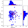 |
Fig. 1. AGN bolometric luminosity (Lbol) as a function of redshift (z) of our sample (red triangles). Also plotted are the known high redshift quasars from the compiled catalogue of Bañados et al. (2016), the catalogue of SDSS detections of Jiang et al. (2016) and the new detections of Mazzucchelli et al. (2017), from which the majority of our sample has been selected. |
As the purpose of this study is to determine the presence of an outflow component, we only included the sample sources where the [C II] line was detected. As a result, we found that 26 sources are detected, and the data are of sufficient quality to be used for the purpose of this paper. This final sample is provided in Table 2.
Results of the observations for the sample sources.
3. ALMA data reduction and analysis
After extracting the [C II] raw data of the 31 quasars from the ALMA archive, we calibrated and imaged (including continuum subtraction) each data set with the Common Astronomy Software Applications1. For about 70% of the sources, a careful manual calibration of the observations was necessary to warrant that the data were calibrated correctly. This was necessary in order to address issues found with flux calibration2, incorrect antenna positions3, low source amplitudes requiring additional flagging, and other issues found in the original calibration. Specifically for the sources with flux calibration issues, we found that the fluxes were wrong by ∼20–45%. For the remaining ∼30% of the sources, the calibration results from the ALMA pipeline were sufficient. For the manually calibrated data sets, we used the CASA software version 5.1.1, to ensure that bugs and calibration issues found for previous CASA versions have been corrected for. Hereafter, a few details are given for each of the archival ALMA projects.
From project 2015.1.00606.S we included two sources (see Table 1). The sources were observed on March 22, 2016, and April 27, 2016. 37 antennas were included in the array with minimum and maximum baselines of 15.3 m and 460.0 m, respectively. Applying natural weighting, the resulting beam size is 0.8″×0.6″. The spectral setup consisted of four spectral windows of 2.0 GHz bandwidth, each containing 128 channels of 15.625 MHz width.
From project 2015.1.00997.S we included five sources (see Table 1). The sources were observed between January and July 2016. Between 37 and 49 antennas were included in the arrays with baselines between 15.1 m and 1.0 km. The synthesised beam sizes resulting from natural weighting ranged between ∼0.4″ and ∼1.2″. The observations were setup with four spectral windows of 1.875 GHz bandwidth each, 480 channels per spectral window, and 3.9 MHz wide channels.
From project 2015.1.01115.S we included 26 sources (see Table 1). The sources were observed between January and June 2016 in arrays with baselines between 15.1 m and 704.1 m. Natural weighting led to synthesised beam sizes between ∼0.4″ and 1.7″. For the spectral setup, 960 channels of 1.953 MHz width covered each of the four 1.875 GHz wide spectral windows. For more extensive details see Decarli et al. (2018).
Finally, all data cubes were imaged to the same angular resolution of 0.8″ × 0.8″ and spectral resolution of 30 km s−1, with a pixel scale of 0.2″. Continuum subtraction was performed using the CASA task UVCONTSUB, using the channels with no line emission. The uncertainty of the absolute flux calibration for all sources falls within 5–10%. For further spectral analysis, the resulting data cubes were imported into the MAPPING software package within GILDAS4. From the continuum-subtracted cubes, we created integrated intensity maps (moment-0) of the [C II] line for each source. With the help of these maps we extracted 1D spectra from the position of the brightest pixel, and the individual areas enclosed by the 2 and 3σ integrated intensity contours (for an example see Fig. 2). We extracted the continuum flux densities (Scont) of each source using a 2D Gaussian fit to the continuum source. The IR (8–1000 μm) luminosity of the sources was estimated by normalising a set of star-forming galaxy templates (from Mullaney et al. 2011, see also Stanley et al. 2018) to the measured Scont values.
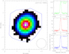 |
Fig. 2. Example for an integrated intensity distribution (moment zero map) and spectra extracted from different regions in J2310+1855. The green box marks the area of the brightest pixel, the area marked by the red line contains all signal above the 3σ threshold, and the blue line outlines the region with signals above 2σ. The spectra extracted from these three regions are shown on the right-hand side. They are colour-coded according to the region from which they were extracted, and the region of extraction is mentioned in the panel for each spectrum as well. On the lower-left side of the image we also show the beam size of our images. |
4. Spectral line stacking techniques
To search for outflow signatures in our sample of z ∼ 6 quasars, we used the spectral stacking analysis tool LINE STACKER (Jolly et al., in prep.). Stacking the [C II] line of the quasars in our sample allows for the search of a broad emission line component, that is weak in comparison to the bright [C II] main line component, and is typically undetected in the individual spectra. We only use the sources where [C II] has been detected, as the detection provides the redshift, and the systemic velocity of the line of each quasar host galaxy.
4.1. Velocity re-binning
To account for the range of line widths (FWHM) observed for the [C II] lines in our sample, we chose to normalise all line widths to the same value. The [C II] lines of all sources were re-binned in channel space with respect to the smallest FWHM measured in the sample, so that each [C II] FWHM is covered by the same number of channels albeit of different channel width. We chose to normalise to the narrowest line and not the widest to avoid oversampling of the data. We note that any sub-samples selected use the re-binned spectra as defined for the full sample. For a [C II] line that has a larger FWHM than the narrowest line, the channels were re-defined to have a width of: cwrebin = cworig × FWHMorig/FWHMmin, where cwrebin is the channel width after re-binning, cworig is the original channel width of 30 km s−1 (see Sect. 3), and FWHMmin is the FWHM of the narrowest line, which corresponds to 270 km s−1.
As a result of the re-binning, the outer velocity bins of the stacked spectrum were not sampled by the same number of sources as the central bins close to the [C II] line core. For the analysis we only considered the central part of the spectrum where the channels include information from the majority of the stacked sample. As we are looking at the mean stacked spectra of the sample, the channel width of the stacked spectrum is taken as the mean channel width of all the individual spectra once re-binned, for our sample that corresponds to 60 km s−1.
4.2. 1D and 3D stacking
In our analysis we performed both 1D and 3D stacking. For the 1D stacking, we first extracted the integrated spectrum for each source, from the region where the moment zero maps have a > 2σ emission. We then re-binned the spectra as described in Sect. 4.1, and stacked. For the 3D stacking, we took the full spectral cubes of each source. Following the method described in Sect. 4.1 we re-binned the full cube using the same parameters determined in our 1D analysis. The cubes were then stacked pixel by pixel in order to create the stacked cube. The stacked cube allows us to extract the stacked spectrum from different regions as well as image different parts of the stacked spectrum.
4.3. Weighting schemes for the line stacking
In our stacking analysis we use three different types of weights (w) when stacking the spectra: (a) w = 1, where the stacks do not include weighting values; (b)  , where
  is the noise; (c) w = 1/Speak, where Speak is the peak flux density of the detected [C II] line.
For case (b) the weight was applied in each velocity channel of the re-binned spectra, using the corresponding noise in that channel. Like this, we took the variations in noise levels of the different observations and spectral channels into account. This is important, as we are interested in the relatively weak outflow component. With the weights of case (c) we normalised for the varying strength of the main component, so that bright lines do not dominate the result.
We repeated our stacking analysis for the three different weighting schemes to search for an outflow component and determine the effects of the varying [C II] line strengths, and noise levels.
5. Results
5.1. Stacking the full sample
In the first column of Fig. 3 we show the 1D stacked spectra for the full sample, for the three different weights used. At the bottom of the figure we also show the number of sources included in each channel. The results from fitting the stacked line are given in Table 3. Including a broad component in the fit improves the χ2 of the fit by 24, 23, and 14% for stacks with weights of w = 1,  , and w = 1/Speak, respectively. However, the fitted parameters for the broad component are not well constrained (see Table 3).
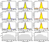 |
Fig. 3. Results from our 1D stacking analysis. Left: stacked spectra of the full sample, middle: max sub-sample, and right: min-sub-sample, using weights of w = 1 (1st row), |

Results of our 1D stacking analysis.
We estimated the significance of the excess emission not accounted for by the single component fit to the line. For this we subtracted the single component fit from the spectrum, and took the sum of the residuals within ±800 km s−1. We find a significance of 0.4–0.7σ, depending on the weighting scheme used (see Table 5).
In Fig. 4 (top panel) we show the stacked cubes of the full sample for the non-weighted stacks. Also shown are the one-component (red) and two-component (blue) fits to the line. The results of the two-component fits to the stacked line are given in Table 4. In the right of Fig. 4 we also show the collapsed image of the wing channels, covering velocities of ±420 − 840 km s−1. In this case, including a broad component improves the χ2 of the fit by 46%, 15%, 34% for weights of w = 1,  , and w = 1/Speak, respectively. Following the methods described earlier, we calculated the significance of the excess emission to be 1.1–1.5σ, depending on the weighting scheme used (see Table 5).
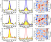 |
Fig. 4. Results from our 3D stacking analysis, for w = 1. From left to right: [C II] line extracted from the stacked cube within a 2″ radius from the centre, a zoom-in view of the broad line component once the narrow component has been removed, combined image of the [C II] line wings from ±420–840 km s−1 (see vertical dotted lines in the spectrum), for the full sample (1st row), the max sub-sample (2nd row), and min sub-sample (3rd row). We also show the one (red curve) and two-component fits (blue solid and dashed curves) to the stacked line. The extent of the narrow component emission is shown with the black contours in the combined images, and the white circle corresponds to the area within a 2″ radius from the centre. |
Results of our 3D stacking analysis.
The 3D stacked line differs to that from our 1D stacking analysis. This is due to the fact that in our 3D stacking analysis we used a larger integration area (2″) than that used in the 1D stacking analysis, where only the area with positive signal was included. Consequently, the 3D stacked line, includes faint extended signal missed by the moment zero 2σ regions used for the 1D stacking analysis. Comparing the results of the 1D stacked spectra with those of the 3D stacked spectra it becomes clear that the broad component in the 1D stacking is poorly constrained, due to the lack of the more extended signal that is included in the 3D stacking.
5.2. A sub-sample with outflow signatures
In addition to simply stacking the full sample in search for an outflow signature, we have also developed a method for determining a sub-sample that maximises the possibility of detecting an outflow signature in the stacked spectrum. Under normal circumstances it is assumed that all stacked sources have the same properties, but in the case of outflows, the orientation of a bi-polar outflow will impact on how it might be detected. If the outflow is oriented in or close to the plane of the sky, the radial component of the velocity will be relatively small and likely remain undetected. This means that even if all sample sources would have a high-velocity outflow, we would expect a fraction of these not to contribute to the stacked signal.
The sub-sample selection was done by randomly selecting sub-sets of n sources, where n is in the range 3−25, and repeated 10 000 times. For each of the 10 000 randomly selected sub-samples, we performed the same stacking analysis as described above. From the resulting stacked spectrum we selected the “line-free” channels, defined to be at a distance of 2 × FWHM from the centre of the main line component. These are channels were we can expect to see only emission due to an outflow component. We then integrated over these channels at different radii from the centre, within the range of 0.2–3″ in steps of 0.2″. The integrated flux density for each integration radius was saved as a grade for the sub-sample.
Once this is done for all 10 000 randomly selected sub-samples, each source in our sample is ranked based on the total sum of the grades of the sub-samples it was in, at all integration radii. Sources with no outflow signal will be mostly in sub-samples with low grades, and will therefore have an overall low rank. We took the mean rank of all sources and defined it as the lower limit for selection of the best sub-sample. The sub-sample of sources selected will be the most likely to have signal from an outflow component (max sub-sample). We also define the sub-sample of least likely sources to have signal from an outflow component (min sub-sample), picked to have a rank below or equal to the mean.
The max sub-sample consists of 12 sources highlighted with boldface in Table 2. We note that the subsampling analysis was performed for both the 1D and 3D stacking analysis and returned the same sub-sample for both cases. These sources cover the same range in bolometric quasar luminosities, redshifts, IR luminosities and [C II] line properties as the full sample (see Fig. 5).
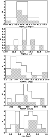 |
Fig. 5. Distribution of the properties of the max sub-sample sources (filled in regions) in comparison to the full sample of this study (main histogram). From top to bottom we compare: the bolometric luminosity of the quasars (Lbol), the IR (8–1000 μm) luminosity of the galaxies (LIR), the Speak, the FWHM, and the rms of the of the individual [C II] lines (before the velocity rebinning). It is evident that the max sub-sample covers a wide range of values in all properties, and is not skewed towards the brightest quasars, specific line-widths or line strength. The max sub-sample does seem to prefer higher rms values, but this is restricted by small number statistics. |
The stacked line of the max sub-sample is shown in the second column of Fig. 3 and the second row of Fig. 4. An outflow component is found in both the 1D and 3D stacking results, for all three weighting schemes. In the case of the 1D stacking analysis we find that the fit when including a broad component, is improved by 48%, 51%, 46% for weights of w = 1,  , and w = 1/Speak, respectively. We find that there is excess emission of 1.1–1.5σ, depending on the weighting scheme used (see Tables 3 and 5). In the case of the 3D stacking analysis the presence of a broad component is more pronounced. We find that including the broad component improves the fit by 62%, 57%, 48% for weights of w = 1,
  , and w = 1/Speak, respectively. Furthermore, the significance of excess emission rises to 1.2–2.5σ (see Tables 4 and 5). The collapsed image (over ±420–840 km s−1) in Fig. 4, shows spatially extended emission, larger than what is seen for the narrow component (see contours), reaching ∼2″.
As discussed earlier, the 3D stacking results are better at constraining the broad component signal compared to the 1D stacking, due to the fact that it includes the more extended faint emission excluded in the 1D stacking. Therefore, for the rest of this paper we only consider the 3D stacking results.
We estimated the mean outflow rate (Ṁoutf) for the max sub-sample, based on the w = 1 3D stacking results. We used the equation of Hailey-Dunsheath et al. (2010) to calculate the outflow gas mass from the integrated [C II] luminosity of the broad component, which includes dependencies on the gas density (n), temperature (T), and abundance of C+ ions (XC+). Following Maiolino et al. (2012) and Cicone et al. (2015), we assumed that XC+ = 1.4 × 10⁻⁴, T = 200 K, and n ≫ ncrit (ncrit ∼ 3 × 103 cm−3), which are typical of photo-dissociated regions. We calculated an estimate of the velocity of the outflow (υoutf) by taking υoutf = 0.5 × FWHM, and took the radius of the extent of the outflow emission (R). By assuming that the velocity of the outflow is constant across the outflow, the dynamical time of the outflow can be defined as τdyn = R/υoutf. Therefore, Ṁoutf = Moutf/τdyn = Moutf × υoutf/R. For the mean redshift of 6.236, a radius of R = 11.5 kpc (2″), and υoutf = 493 km s−1, we find that Ṁoutf = 45 ± 21 M⊙ yr−1. Since the properties of the broad component do not change significantly for the different weights, the calculated mass outflow rate will be similar for all weights.
To determine if a specific source in our max sub-sample is driving the outflow component emission or the shape of the extended emission, we performed a test. We repeated our stacking analysis as many times as the number of sources in the max sub-sample, and each time removed one of the sources. As a result we have the stacked lines and collapsed images for each source’s exclusion from the sub-sample. If one source is driving the observed results of the max sub-sample, then the stack without it will show significant differences to that of the max sub-sample. We find that none of the sources cause a significant difference in the extent of the high-velocity emission seen in the collapsed images, and none are specifically driving the shape and strength of the outflow component of the stacked [C II] line. Specifically, the FWHM, Speak values of the broad component remain within 20% of those found for the stack of the complete max sub-sample, and remain within the error of the fitted values (see Table 4).
If we extract the line only from the central pixel then there is no evidence for an outflow, in agreement with the results by Decarli et al. (2018). Taking the central pixel is equivalent to taking the flux within the beam for point like sources. This suggests that the emission of the outflow is spatially extended beyond the beam, as indicated by the collapsed image of the line wings in Fig. 4.
We have also looked into the stack of the sources excluded from the max sub-sample described above (right column of Fig. 3 and lower row of Fig. 4). A stack for these sources shows no evidence of an outflow component, and the line wing images show no significant traces of emission. This result also adds to the reasonableness of our max sub-sample selection, since it does not show any outflow signal, but also the average signal is not negative which could be the case if the signal in the max sub-sample was artificial.
In this analysis we have assumed that the outflow emission signature has the spectral profile of a single broad Gaussian, which might not be the case for some or all of the quasars in our sample. Previous individual detections of outflows reported in the literature using e.g., CO, HCN, or [C II], show that the majority of the lines have nearly symmetric, broad emission lines, with a subset of results showing outflows dominated by emission only on the red or blue side of the main component (e.g., Cicone et al. 2014; Janssen et al. 2016). Apparent individual emission line components with a high velocity offset from the dominant line component could also be interpreted as an outflow signature (e.g., Fan et al. 2018). Furthermore, we have assumed that the broad component found is originating from the high-velocity gas of an outflow. However, it is possible that the high-velocity emission is not due to an outflow but for example, a gas flow between two interacting galaxies (for a detailed discussion see Gallerani et al. 2018). We know of one source included in our sample (PJ308−21) that has complex high-velocity structure (e.g. Decarli et al. 2017). However, when this source is removed from our stacking analysis, the observed broad component and the spatial extent of the wings do not change significantly.
5.3. Testing the feasibility of detecting an outflow signal with our method
To determine if the methods of our analysis are indeed capable of detecting an outflow component, we test their performance on mock samples with and without an outflow component. To test if our method can successfully retrieve the broad component signal, we performed our 1D stacking analysis on a mock sample with [C II] lines that included a weak broad component. Based on the extracted spectra of our observed sample, we used the one-component line fits of the observed lines, to which we added a broad line component of similar properties to what we find in our stacking results, with 2 times the width and 0.1 times the peak flux density of the main line component. For 10 000 iterations, we added random noise to the individual [C II] lines, based on the range of the observed rms, and stacked following our 1D stacking analysis. We then determined if we could detect excess emission due to a broad component in the stacked spectra, following the method described in Sect. 5.1. We find excess emission due to a broad component with only a weak significance of < 3σ, with 75% of iterations having an excess emission of 1 − 2σ for stacks with weights of w = 1 and  . However, a weight of w = 1/Speak seems to suppress the signal, with the detectability of excess emission dropping to 20% for a 1 − 2σ significance (see figures in Appendix A). It is worth noting however, that if assuming a stronger initial broad component, with 3 times the width and 0.2 times the peak flux density of the main line component, then our method retrieves a strong broad component in the stacks. In this case an excess emission of > 5σ for > 99% of iterations, for stacks with weights of w = 1 and
  , and > 3σ for 35% of iterations for w = 1/Speak.
To test if it is possible that the outflow component found in our results could be created by stacked noise and is not a real signal, we performed a similar test. Based on the one-component fit to the [C II] lines of our sample, we created a mock sample with the same line properties, and without an added outflow component. We then added random noise to each, based on the range of the observed rms. We performed our 1D stacking analysis on this mock sample 10 000 times, each time re-applying randomly selected noise levels. Then we attempted a two-component fit to each stacked line and determined if a broad line component is found and if it has comparable properties to the one found in our analysis of the observed data. This is done for all three weighting schemes. We find that, depending on the weight scheme used, 14–17% of the iterations return a > 0.4σ excess signal in the stacked lines (see Appendix A).
6. Discussion
6.1. Spectral line stacking methods
At the high redshifts covered in our study the spatial information available is limited. Therefore, our analysis will primarily be sensitive to the information that can be derived from the velocity characteristics of the observed lines. Hence our type of analysis is relevant for outflows that have velocities higher than that of the host galaxy emission, and low-velocity outflows will not be detected.
As the aim of the stacking is to search for a faint broad emission line component, it is imperative to understand the effect of stacking data where the main (bright) component has varying line widths. If spectral lines, such as those of the data used here, are simply stacked, it could result in the detection of an artificial broad component. To test the effect of the varying FWHM values of the lines stacked on the final result, we created a mock sample with the line properties of the observed sample, without adding an outflow component. We performed our stacking analysis on this mock sample 10 000 times, each time re-applying randomly selected noise levels within the range of observed rms. For each iteration we performed both straightforward stacking, and stacking using our rebinning method. For the resulting stacked spectra we attempt two-component fitting to determine if a significant broad component is found. We find that for the straightforward stacking analysis, excess emission due to a broad component is found at > 2σ 2–5% of the time. However, we find that these cases are due to the noise of the stacked spectrum. If we repeat the exercise without including noise in the spectra, then a broad component is not found. It is worth noting that even if a significant broad component is not fitted in the majority of the cases, there is still low significance (< 1σ) excess emission in the line wings that the single component gaussian cannot fit (see examples in Appendix A).
Recently, there have been two other studies looking at similar samples of high-z quasars with [C II] (Decarli et al. 2018; Bischetti et al. 2019). In Decarli et al. (2018) a sample of z ∼ 6 quasars observed with [C II] is presented, and a brief analysis on the presence of outflows is included. The overall analysis is not that different to our own, as they also use velocity rebinning before stacking, but have only stacked the spectra extracted from the central pixel of each source. They report no evidence for a broad component in the stacked spectra, which is consistent with the results of our 1D stacking analysis of the full sample. However, as we have demonstrated in this paper, it is imperative to take into account the emission from the entire extent of the galaxy, as the outflow emission may be originating from an extended region.
Bischetti et al. (2019) use archival data of quasars in the wider redshift range of 4.5 < z < 7.1, to search for outflow signatures in the stacked spectra. However, it is not clear how the archive data have been treated; as noted previously, we needed to manually re-calibrate 70% of the archive observations of our sample. The individual spectra were integrated over a region equivalent of four times the beam size, and were stacked without velocity rebinning but with a weighting scheme of  for each channel of each spectrum. Evidence for a broad outflow component are found, in agreement with our conclusions, but with a stronger significance. The higher significance of the broad component found in the Bischetti et al. (2019) analysis could be due to the absence of velocity rebinning to account for the range in the FWHM values of the lines stacked, which could result to an overestimate of the flux and FWHM of the broad component. However, it could also be due to the larger sample used in their analysis.
Even though velocity re-binning is important in order to not introduce artificial signal to the broad line emission, it also implies that the line width of the broad line component is roughly proportional to that of the main component. Consequently, our analysis can detect a broad component, but it will not be based on the absolute value of the line width, but rather on the mean of the velocity axis of the spectra stacked. However, current available spectroscopic data lack the sensitivity to fully detect individual outflows, and spectral stacking is the only available method at present to determine the presence of outflow signatures.
6.2. Should we expect to see outflows in all high-z quasars?
As discussed previously, we find only a tentative signal for an outflow component when stacking the full sample of z ∼ 6 quasars, but find that for a specific subsample of sources we can detect a significant outflow component. This would suggest that either not all z ∼ 6 quasars have outflows (at least at the time of observation), or there are effects that inhibit the observability of present outflows.
Recently, a study by Barai et al. (2018) using zoom-in hydrodynamical simulations to determine the effect of outflows on the host galaxy and surrounding environment of quasars at z ≥ 6, has demonstrated that outflows could indeed be a dominant feature of high redshift quasars. Even though the quasar host galaxies at z ∼ 6 are accreting significant amounts of cosmic gas, AGN feedback succeeds in reducing the inflow by ∼12%, with ∼20% of the quasar outflows having speeds greater than the escape velocity of 500 km s−1, subsequently succeeding in ejecting gas out of the host galaxy, and regulating the on-going star formation (Barai et al. 2018).
6.2.1. Outflow orientation
The presence, strength, and width of a broad line component due to outflow emission are dependent on the orientation of the outflow with respect to the observer’s line of sight. Indeed, in a recent study by Roberts-Borsani & Saintonge (2019) investigating cold gas inflows and outflows around galaxies in the local Universe, it was found that outflows were detected only for outflow angles < 50° in respect to the line of sight, while for > 60° it was only possible to detect inflows.
To test how orientation angles could affect the observability of an outflow component in the stacked spectra we ran a simple Monte-Carlo test. In its most simplistic form, we assumed that all galaxies in the sample have the same values of peak flux density and FWHM of their lines and have the same outflow component.
We first defined a line profile that is a combination of a narrow and broad component. For the narrow component we assumed Speak = 10 mJy and FWHM = 400 km s−1. For the broad component, we assumed five different FWHM values (800, 900, 1000, 1100, 1200 km s−1) and repeated the test for each.
For each of the broad component FWHM values, we ran 1000 iterations, in each of which we selected 30 random angles between 10–80° (simplistic assumption to avoid a blazar, 0°, and obscured quasar, 90°, types). We combined the selected random orientation angles with the defined line profile to create a mock sample of 30 galaxies, and added random noise with rms of ∼0.5 mJy, similar to what is seen in the observed sample. We then stacked the spectra following the same methods as described in Sect. 4. We fitted the resulting stacked spectral line with a single and double-component Gaussian function, and calculated the respective χ2 values of the fits, and the significance of the broad component emission.
We find that an excess emission due to a broad component, of > 2σ significance is retrieved for 27 − 50% of the iterations, for the cases where we had assumed an initial broad component with FWHM > 1000 km s−1. For an initial broad component with FWHM of 800 and 900 km s−1, a broad component in the stack with > 1σ is found in > 60% of iterations (see Figs. A.2 and A.4).
6.2.2. Choice of outflow tracers
The choice of a tracer is an important part in all studies aiming to determine the presence and properties of outflows in galaxies. The recent studies on the presence of outflows in the most distant quasars (this work; Decarli et al. 2018; Bischetti et al. 2019) all show different results, and none can reproduce the very strong signal seen in SDSS J1148+5251 (e.g. Cicone et al. 2015). Therefore, it is important to consider if [C II] is indeed a suitable tracer of outflows.
[C II] 158 μm is a tracer of atomic gas at typical densities of 2.8 × 103 cm−3 with temperatures of ∼92 K. It conveniently falls within the ALMA bands at z ∼ 6, and therefore is easy to observe and proves a very useful tracer, especially for quasar studies (see review by Carilli & Walter 2013). However, at lower redshifts, there is a variety of more commonly used gas tracers for the detection of outflow signatures of AGN, such as 12CO tracing molecular gas.
[C II] emission can originate from ionised, atomic, and molecular regions; however, both low and high redshift observational and theoretical work argue that the majority of [C II] emission (70–90%) originates from neutral atomic gas (e.g., Croxall et al. 2017; Olsen et al. 2015; Lagache et al. 2018). Although, there has been observational evidence of [C II] emission from ionised regions (e.g., Contursi et al. 2013; Decarli et al. 2014). [C II] emission has also been found to trace molecular gas that is “CO-faint” due to the disassociation of the CO molecules from far-unltraviolet emission (e.g., Jameson et al. 2018). However, Lagache et al. (2018) highlight that the [C II] emission at redshifts z > 6 can be strongly affected by attenuation from the cosmic microwave background; although it is mostly warm and low density gas that is affected by this. [C II] 158 μm has been successful in detecting outflows in a few nearby galaxies (e.g., Contursi et al. 2013; Kreckel et al. 2014), but at redshifts of z ∼ 6 the only example of a quasar outflow detected with [C II] is J1148+5251 (e.g., Maiolino et al. 2012; Cicone et al. 2015).
It is possible that CO cannot survive in the outflow regions; however, CO(5-4) has been seen in an ionised outflow region (e.g., Brusa et al. 2018, similar result found in Fogasy et al., in prep.) at high redshifts, and there are plenty of nearby galaxies with resolved molecular outflows traced with multiple CO transitions (e.g., Alatalo et al. 2011; Aalto et al. 2012; Cicone et al. 2012, 2014; Feruglio et al. 2015; Veilleux et al. 2013, 2017).
Although Hα and [O III], as well as X-ray emission can directly trace the shocked and ionised regions caused by the outflows, and hence may be a more direct probe, such observations are currently impossible at such high redshifts. There is currently only one tentative detection of hot gas in the X-ray (SDSS J1030+0524, Nanni et al. 2018). However, future JWST projects may be able to probe the ionised gas in high redshift outflows.
Overall, due to the lack of systematic studies on the topic it remains unclear if [C II] – so far the most commonly studied outflow tracer at high-z – is a good tracer of outflows in distant galaxies. However, with the sensitivity of ALMA it is possible to have systematic studies in the future, to address this.
6.3. The presence of outflows in high-redshift quasars.
Individual studies of high-redshift quasars have revealed some evidence for outflows based on [C II] and CO observations. At a redshift of z ∼ 6.4, the luminous quasar SDSS J1148+5251 shows a strong [C II] broad component indicating the presence of an outflow with velocities of up to 1400 km s−1 and extending to distances of ∼30 kpc (Maiolino et al. 2012; Cicone et al. 2015). At the lower redshifts of z ∼ 1.4, z ∼ 1.6, and z ∼ 3.9, Vayner et al. (2017), Brusa et al. (2018), and Feruglio et al. (2017) report the detection of a molecular outflow traced with CO. In the first two cases the outflow velocities are 600–700 km s−1, while in the third case the outflow velocity reaches up to ∼1300 km s−1. At redshifts of z ∼ 1 − 3 there are also numerous detections of ionised outflows traced with [O III] (e.g., Harrison et al. 2012, 2016; Brusa et al. 2016; Carniani et al. 2016; Vayner et al. 2017).
In studies of lower redshift AGN outflows of z < 0.2 using [O III] ionised gas tracer, there is a prevalence of outflows in both luminous AGN (e.g., Harrison et al. 2014) and among ULIRGs hosting AGN (e.g., Rose et al. 2018; Tadhunter et al. 2018; Spence et al. 2018), with typical line widths of ≃600 − 1500 km s−1 and ≃500 − 2500 km s−1. Similarly, molecular outflow studies of nearby quasar galaxies using CO, HCN, and other molecular tracers, have found outflows with velocities reaching ≃750 − 1100 km s−1 (e.g., Cicone et al. 2014; Aalto et al. 2015; Veilleux et al. 2017).
For the max sub-sample we find a mean outflow velocity of ∼387–713 km s−1, consistent with observations of both ionised and molecular outflows in single objects up to z ∼ 2.5. Our results are also consistent with the range of mean outflow velocities reported in Bischetti et al. (2019). We find that the ratio of the peak flux densities of the outflow over the main component, found for our full sample and max-subsample, ranges between ≃0.1 and 0.5 for both, and is highly dependent on the weighting scheme used. This is in agreement with the relative ratio of 0.14 seen in J1148+5251 at z ∼ 6 (e.g., Maiolino et al. 2005; Cicone et al. 2015), while larger than seen in Mrk231 (≃0.067) when using the different tracer CO(1-0) in the nearby Mrk231 (e.g., Cicone et al. 2012).
In order to improve our understanding on the prevalence of outflows at z ∼ 6 and above we will need deeper observations of quasar samples in both [C II] and CO, as well as tracers of the warm ionised medium. However, a multi-tracer approach is costly in terms of observing time, and thus the methods presented in this work provide a useful step towards designing the relevant observations. Large emission line surveys of high-redshift quasars can be combined with the sub-sampling method presented in Sect. 5.2, to determine the more likely candidates to have outflows for deeper multi-phase observations. Apart from the ability to select a sub-sample of most likely sources to have an outflow, sub-sampling can also help to take into account potential effects such as orientation or selection effects.
7. Conclusions
We have carried out a study of spectral stacking of [C II] ALMA archive observations for z ∼ 6 optically selected quasars, to search for faint outflow signal. We performed this analysis for both extracted spectra and full spectral cubes, allowing for the extraction of stacked spectra over different regions. We also performed a sub-sampling technique to identify the sub-sample of our sources that maximise the broad component signal when stacked.
Specifically:
-
We find tentative broad component signal for our full sample of 26 quasars. The stacked spectrum has a broad component of FWHM > 700 km s−1 with a total line flux density of Sint > 0.5 Jy km s−1. The excess emission, above a single component fit to the stacked line, corresponds to 0.4–1.5σ, depending on the weighting scheme used in the stack.
-
We identify a sub-sample of 12 sources, which maximise the broad component signal when stacked. The broad component detected in this sub-sample is characterised by an average FWHM > 775 km s−1, and Sint > 1.2 Jy km s−1. The excess emission is detected at 1.2–2.5σ, depending on the weighting scheme used. These results are consistent with results of individual sources at low and high redshifts.
-
We test if our methods could introduce artificial outflow signal when stacking, by creating mock samples based on the observed [C II] line properties of our sample. In these mock samples there is no broad component included. We find that the probability to falsely detect a broad component with an excess emission of > 0.4σ is < 17%.
Using spectral line stacking as a tool for this type of studies has the following implications:
-
Spectral line stacking is a meaningful tool for searching for outflows in the spectra of quasars. Given that the redshift is well known because of the bright line emission from the host galaxies, there will be no significant velocity offsets that would dilute the emission from the fainter (broad) component. However, it is important to take into account the varying line width of the main line component in order to avoid introducing additional broad spectral features.
-
As outflows are thought to be anisotropic emission that is typically seen as bi-polar, and for which the orientation is most likely random, it is expected that at least a sub-set of the sample will not contribute significant, or any, emission from the outflow to the stacked spectrum. For instance, if the outflow is aligned close to or on the line of sight, the projected radial velocity might be the same or less than that of the main component. For a sample typically of the size studied here, if the orientation is random, it would be possible to obtain an outflow signal if the outflow velocity is larger than twice the main component line width. To take into account the fact that not all sources will be contributing significantly, we developed a tool for identifying the sub-sample most likely to have outflow signatures in its stacked spectrum.
-
We have used the assumption that the outflow is characterised by a high velocity component with a line width significantly larger than that of main line, and such spectral signatures are seen in some local AGNs that have detected outflows. However, it is possible that outflows may have other spectral characteristics, that will not be traced with our methods.
This type of study represents a step towards better insights in outflows and possible feedback in massive galaxies. However, to gain full insights the next steps will need to include direct detection of individual sources as well as the detection of multiple outflow tracers.
This is the case for sources originally calibrated with CASA version 4.6 or prior with the sources Ceres or Pallas as their flux calibrators. Through private communication with the ALMA Nordic ARCnode it was pointed out to us that for those versions of CASA the flux models for Pallas and Ceres were wrong. Consequently, the fluxes extrapolated for the sources observed with Ceres or Pallas as flux calibrators will be wrong without re-calibration.
In these cases the data were observed right after a shift in the antenna positions but did not have the new correct coordinates when the original calibration was performed. We have made sure to use the correct coordinates.
Acknowledgments
We thank the anonymous referee for their instructive comments for the improvement of this paper. FS acknowledges support from the Nordic ALMA Regional Centre (ARC) node based at Onsala Space Observatory. The Nordic ARC node is funded through Swedish Research Council grant No. 2017–00648. KK acknowledges support from the Swedish Research Council and the Knut and Alice Wallenberg Foundation. This paper makes use of the following ALMA data: ADS/JAO.ALMA#2015.0.00606.S, ADS/JAO.ALMA#2015.0.00997.S, ADS/JAO.ALMA#2015.0.01115.S. ALMA is a partnership of ESO (representing its member states), NSF (USA) and NINS (Japan), together with NRC (Canada), MOST and ASIAA (Taiwan), and KASI (Republic of Korea), in cooperation with the Republic of Chile. The Joint ALMA Observatory is operated by ESO, AUI/NRAO and NAOJ. This research made used of APLpy, an open-source plotting package for Python (Robitaille & Bressert 2012).
References
- Aalto, S., Garcia-Burillo, S., Muller, S., et al. 2012, A&A, 537, A44 [NASA ADS] [CrossRef] [EDP Sciences] [Google Scholar]
- Aalto, S., Martín, S., Costagliola, F., et al. 2015, A&A, 584, A42 [NASA ADS] [CrossRef] [EDP Sciences] [Google Scholar]
- Alatalo, K., Blitz, L., Young, L. M., et al. 2011, ApJ, 735, 88 [NASA ADS] [CrossRef] [Google Scholar]
- Bañados, E., Venemans, B. P., Morganson, E., et al. 2014, AJ, 148, 14 [NASA ADS] [CrossRef] [Google Scholar]
- Bañados, E., Venemans, B. P., Decarli, R., et al. 2016, ApJS, 227, 11 [NASA ADS] [CrossRef] [Google Scholar]
- Barai, P., Gallerani, S., Pallottini, A., et al. 2018, MNRAS, 473, 4003 [NASA ADS] [CrossRef] [Google Scholar]
- Barcos-Muñoz, L., Aalto, S., Thompson, T. A., et al. 2018, ApJ, 853, L28 [NASA ADS] [CrossRef] [Google Scholar]
- Bischetti, M., Maiolino, R., Fiore, S. C. F., Piconcelli, E., & Fluetsch, A. 2019, A&A, 630, A59 [NASA ADS] [CrossRef] [EDP Sciences] [Google Scholar]
- Brusa, M., Perna, M., Cresci, G., et al. 2016, A&A, 588, A58 [NASA ADS] [CrossRef] [EDP Sciences] [Google Scholar]
- Brusa, M., Cresci, G., Daddi, E., et al. 2018, A&A, 612, A29 [NASA ADS] [CrossRef] [EDP Sciences] [Google Scholar]
- Carilli, C. L., & Walter, F. 2013, ARA&A, 51, 105 [NASA ADS] [CrossRef] [EDP Sciences] [Google Scholar]
- Carnall, A. C., Shanks, T., Chehade, B., et al. 2015, MNRAS, 451, L16 [NASA ADS] [CrossRef] [Google Scholar]
- Carniani, S., Marconi, A., Maiolino, R., et al. 2016, A&A, 591, A28 [NASA ADS] [CrossRef] [EDP Sciences] [Google Scholar]
- Cicone, C., Feruglio, C., Maiolino, R., et al. 2012, A&A, 543, A99 [NASA ADS] [CrossRef] [EDP Sciences] [Google Scholar]
- Cicone, C., Maiolino, R., Sturm, E., et al. 2014, A&A, 562, A21 [NASA ADS] [CrossRef] [EDP Sciences] [Google Scholar]
- Cicone, C., Maiolino, R., Gallerani, S., et al. 2015, A&A, 574, A14 [NASA ADS] [CrossRef] [EDP Sciences] [Google Scholar]
- Contursi, A., Poglitsch, A., Grácia Carpio, J., et al. 2013, A&A, 549, A118 [NASA ADS] [CrossRef] [EDP Sciences] [Google Scholar]
- Croxall, K. V., Smith, J. D., Pellegrini, E., et al. 2017, ApJ, 845, 96 [NASA ADS] [CrossRef] [Google Scholar]
- Decarli, R., Walter, F., Carilli, C., et al. 2014, ApJ, 782, L17 [NASA ADS] [CrossRef] [Google Scholar]
- Decarli, R., Walter, F., Venemans, B. P., et al. 2017, Nature, 545, 457 [NASA ADS] [CrossRef] [Google Scholar]
- Decarli, R., Walter, F., Venemans, B. P., et al. 2018, ApJ, 854, 97 [NASA ADS] [CrossRef] [Google Scholar]
- De Rosa, G., Decarli, R., Walter, F., et al. 2011, ApJ, 739, 56 [NASA ADS] [CrossRef] [Google Scholar]
- Fabian, A. C. 2012, ARA&A, 50, 455 [NASA ADS] [CrossRef] [Google Scholar]
- Fan, L., Knudsen, K. K., Fogasy, J., & Drouart, G. 2018, ApJ, 856, L5 [NASA ADS] [CrossRef] [Google Scholar]
- Fan, X., Narayanan, V. K., Lupton, R. H., et al. 2001, AJ, 122, 2833 [NASA ADS] [CrossRef] [Google Scholar]
- Fan, X., Strauss, M. A., Richards, G. T., et al. 2006, AJ, 131, 1203 [NASA ADS] [CrossRef] [Google Scholar]
- Feruglio, C., Fiore, F., Carniani, S., et al. 2015, A&A, 583, A99 [NASA ADS] [CrossRef] [EDP Sciences] [Google Scholar]
- Feruglio, C., Ferrara, A., Bischetti, M., et al. 2017, A&A, 608, A30 [NASA ADS] [CrossRef] [EDP Sciences] [Google Scholar]
- Gallerani, S., Pallottini, A., Feruglio, C., et al. 2018, MNRAS, 473, 1909 [NASA ADS] [CrossRef] [Google Scholar]
- Hailey-Dunsheath, S., Nikola, T., Stacey, G. J., et al. 2010, ApJ, 714, L162 [NASA ADS] [CrossRef] [Google Scholar]
- Harrison, C. M., Alexander, D. M., Swinbank, A. M., et al. 2012, MNRAS, 426, 1073 [NASA ADS] [CrossRef] [Google Scholar]
- Harrison, C. M., Alexander, D. M., Mullaney, J. R., & Swinbank, A. M. 2014, MNRAS, 441, 3306 [Google Scholar]
- Harrison, C. M., Alexander, D. M., Mullaney, J. R., et al. 2016, MNRAS, 456, 1195 [NASA ADS] [CrossRef] [Google Scholar]
- Jameson, K. E., Bolatto, A. D., Wolfire, M., et al. 2018, ApJ, 853, 111 [NASA ADS] [CrossRef] [Google Scholar]
- Janssen, A. W., Christopher, N., Sturm, E., et al. 2016, ApJ, 822, 43 [NASA ADS] [Google Scholar]
- Jiang, L., McGreer, I. D., Fan, X., et al. 2015, AJ, 149, 188 [NASA ADS] [CrossRef] [Google Scholar]
- Jiang, L., McGreer, I. D., Fan, X., et al. 2016, ApJ, 833, 222 [NASA ADS] [CrossRef] [Google Scholar]
- King, A., & Pounds, K. 2015, ARA&A, 53, 115 [Google Scholar]
- Knudsen, K. K., Richard, J., Kneib, J.-P., et al. 2016, MNRAS, 462, L6 [NASA ADS] [CrossRef] [Google Scholar]
- Kreckel, K., Armus, L., Groves, B., et al. 2014, ApJ, 790, 26 [NASA ADS] [CrossRef] [Google Scholar]
- Kurk, J. D., Walter, F., Fan, X., et al. 2007, ApJ, 669, 32 [NASA ADS] [CrossRef] [Google Scholar]
- Lagache, G., Cousin, M., & Chatzikos, M. 2018, A&A, 609, A130 [NASA ADS] [CrossRef] [EDP Sciences] [Google Scholar]
- Maiolino, R., Cox, P., Caselli, P., et al. 2005, A&A, 440, L51 [NASA ADS] [CrossRef] [EDP Sciences] [Google Scholar]
- Maiolino, R., Gallerani, S., Neri, R., et al. 2012, MNRAS, 425, L66 [NASA ADS] [CrossRef] [Google Scholar]
- Matsuoka, Y., Onoue, M., Kashikawa, N., et al. 2016, ApJ, 828, 26 [NASA ADS] [CrossRef] [Google Scholar]
- Mazzucchelli, C., Bañados, E., Venemans, B. P., et al. 2017, ApJ, 849, 91 [NASA ADS] [CrossRef] [Google Scholar]
- McMullin, J. P., Waters, B., Schiebel, D., Young, W., & Golap, K. 2007, in Astronomical Data Analysis Software and Systems XVI, eds. R. A. Shaw, F. Hill, & D. J. Bell, ASP Conf. Ser., 376, 127 [Google Scholar]
- Mortlock, D. J., Patel, M., Warren, S. J., et al. 2009, A&A, 505, 97 [NASA ADS] [CrossRef] [EDP Sciences] [Google Scholar]
- Mullaney, J. R., Alexander, D. M., Goulding, A. D., & Hickox, R. C. 2011, MNRAS, 414, 1082 [NASA ADS] [CrossRef] [Google Scholar]
- Nanni, R., Gilli, R., Vignali, C., et al. 2018, A&A, 614, A121 [NASA ADS] [CrossRef] [EDP Sciences] [Google Scholar]
- Olsen, K. P., Greve, T. R., Narayanan, D., et al. 2015, ApJ, 814, 76 [CrossRef] [Google Scholar]
- Omont, A., Willott, C. J., Beelen, A., et al. 2013, A&A, 552, A43 [NASA ADS] [CrossRef] [EDP Sciences] [Google Scholar]
- Reed, S. L., McMahon, R. G., Banerji, M., et al. 2015, MNRAS, 454, 3952 [NASA ADS] [CrossRef] [Google Scholar]
- Roberts-Borsani, G. W., & Saintonge, A. 2019, MNRAS, 482, 4111 [NASA ADS] [Google Scholar]
- Robitaille, T., & Bressert, E. 2012, Astrophysics Source Code Library [record ascl:1208.017] [Google Scholar]
- Rose, M., Tadhunter, C., Ramos Almeida, C., et al. 2018, MNRAS, 474, 128 [Google Scholar]
- Runnoe, J. C., Brotherton, M. S., & Shang, Z. 2012, MNRAS, 426, 2677 [NASA ADS] [CrossRef] [Google Scholar]
- Rupke, D. S. N., & Veilleux, S. 2011, ApJ, 729, L27 [NASA ADS] [CrossRef] [Google Scholar]
- Schaye, J., Crain, R. A., Bower, R. G., et al. 2015, MNRAS, 446, 521 [Google Scholar]
- Sijacki, D., Vogelsberger, M., Genel, S., et al. 2015, MNRAS, 452, 575 [NASA ADS] [CrossRef] [Google Scholar]
- Somerville, R. S., Hopkins, P. F., Cox, T. J., Robertson, B. E., & Hernquist, L. 2008, MNRAS, 391, 481 [NASA ADS] [CrossRef] [Google Scholar]
- Spence, R. A. W., Tadhunter, C. N., Rose, M., & Rodríguez Zaurín, J. 2018, MNRAS, 478, 2438 [NASA ADS] [CrossRef] [Google Scholar]
- Stanley, F., Harrison, C. M., Alexander, D. M., et al. 2018, MNRAS, 478, 3721 [NASA ADS] [CrossRef] [Google Scholar]
- Sturm, E., González-Alfonso, E., Veilleux, S., et al. 2011, ApJ, 733, L16 [NASA ADS] [CrossRef] [Google Scholar]
- Tadhunter, C., Rodríguez Zaurín, J., Rose, M., et al. 2018, MNRAS, 478, 1558 [NASA ADS] [CrossRef] [Google Scholar]
- Vayner, A., Wright, S. A., Murray, N., et al. 2017, ApJ, 851, 126 [NASA ADS] [CrossRef] [Google Scholar]
- Veilleux, S., Meléndez, M., Sturm, E., et al. 2013, ApJ, 776, 27 [NASA ADS] [CrossRef] [Google Scholar]
- Veilleux, S., Bolatto, A., Tombesi, F., et al. 2017, ApJ, 843, 18 [Google Scholar]
- Venemans, B. P. 2017, The Messenger, 169, 48 [NASA ADS] [Google Scholar]
- Venemans, B. P., McMahon, R. G., Walter, F., et al. 2012, ApJ, 751, L25 [Google Scholar]
- Venemans, B. P., Bañados, E., Decarli, R., et al. 2015, ApJ, 801, L11 [NASA ADS] [CrossRef] [Google Scholar]
- Venemans, B. P., Walter, F., Zschaechner, L., et al. 2016, ApJ, 816, 37 [NASA ADS] [CrossRef] [Google Scholar]
- Venemans, B. P., Walter, F., Decarli, R., et al. 2017, ApJ, 845, 154 [NASA ADS] [CrossRef] [Google Scholar]
- Venemans, B. P., Decarli, R., Walter, F., et al. 2018, ApJ, 866, 159 [NASA ADS] [CrossRef] [Google Scholar]
- Wang, R., Wagg, J., Carilli, C. L., et al. 2011, ApJ, 739, L34 [NASA ADS] [CrossRef] [Google Scholar]
- Wang, R., Wagg, J., Carilli, C. L., et al. 2013, ApJ, 773, 44 [NASA ADS] [CrossRef] [Google Scholar]
- Wang, R., Wu, X.-B., Neri, R., et al. 2016, ApJ, 830, 53 [NASA ADS] [CrossRef] [Google Scholar]
- Willott, C. J., Delorme, P., Omont, A., et al. 2007, AJ, 134, 2435 [NASA ADS] [CrossRef] [Google Scholar]
- Willott, C. J., Delorme, P., Reylé, C., et al. 2010, AJ, 139, 906 [NASA ADS] [CrossRef] [Google Scholar]
- Willott, C. J., Omont, A., & Bergeron, J. 2013, ApJ, 770, 13 [NASA ADS] [CrossRef] [Google Scholar]
- Willott, C. J., Bergeron, J., & Omont, A. 2017, ApJ, 850, 108 [NASA ADS] [CrossRef] [Google Scholar]
Appendix A: Tests on the spectral stacking methods and orientation effects
In Sect. 5.3 we discussed two tests on the spectral stacking analysis using mock samples. One where all the lines in our mock sample included a broad component bellow the noise, and one where no broad component was included in the mock sample. Here we show the fraction of iterations showing excess emission due to a broad component at different significance levels (Fig. A.1), and example stacked spectra from these tests (Fig. A.3). As discussed in Sect. 5.3, our spectral stacking analysis successfully retrieves a broad component in the stacked lines of the mock samples with an outflow component 75% of the time, with an excess emission of 1 − 2σ for weights of w = 1 and  . But for w = 1/Speak, its only able to retrieve excess emission at 1 − 2σ 20% of the time. In the case of the mock samples without an outflow component included, there is no excess emission detected at > 2σ, and only < 17% of the time do we retrieve excess emission between 0.4 and 2σ.
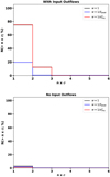 |
Fig. A.1. Histogram of the fraction of iterations that the stacked spectra shows excess emission at significance levels greater than n × σ. Top: results of our test on stacking mock samples where all sources had a broad component below the noise levels. Bottom: results of our test on stacking mock samples where all sources had no added broad component. We show the results for stacking with all three of the weights assumed in this work. |
In Sect. 6.1 we discussed the effect of stacking lines without taking into account the range of line widths of the sample, by not applying velocity rebinning on the lines before stacking. In this case we did a test on stacking a mock sample of lines with similar properties to our sample and with no broad component, without applying velocity rebinning. We repeated the exercise with and without the inclusion of noise in the mock samples. If there is no noise included, the stacked line does not have a broad component in any of the iterations. When including the noise, we retrieve > 2σ excess emission only 2–5% of the time. We show examples of the stacked spectra from this test in Fig. A.3 (last row).
In Sect. 6.2.1 we discussed the effect that the orientation of the outflows could have on the detections of a broad component signature in the stacked lines (see Sect. 6.2.1). In Fig. A.2 we show the fraction of iterations with excess emission in the stack at different significance levels, for each of the assumed initial FWHM of the broad component (800, 900, 1000, 1100, 1200 km s−1). We find that for initial broad components with FWHM > 900 km s−1, we can retrieve excess emission of > 1σ, while we can retrieve a > 2σ signal only for initial broad components with FWHM > 1100 km s−1 ∼27–50% of the time. Example spectra from this test are shown in Fig. A.4.
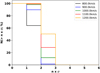 |
Fig. A.2. Histogram of the fraction of iterations that the stacked spectra shows excess emission at significance levels greater than n × σ. In this case we show the results of our outflow orientation test. Each colour corresponds to a different initial FWHM of the broad component. |
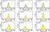 |
Fig. A.3. Top: example spectra from the test on stacking mock samples where all sources had a broad component below the noise levels, for each of the different weights usedd. Also given are the significance values of the excess emission due to a broad component, for each example. Middle: example spectra from the test on stacking mock samples where all sources had no added broad component. Bottom: example spectra from the test on stacking mock samples where all sources had no added broad component, but without using velocity re-binning. We also show the one (red curve) and two-component fits (blue solid and dashed curves) to the stacked lines. |
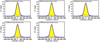 |
Fig. A.4. Example spectra from the orientation test, for each of the different initial broad component FWHM values. We also show the one (red curve) and two-component fits (blue solid and dashed curves) to the stacked lines. |
All Tables
Properties for our sample of z ∼ 6 quasars available in the ALMA archive by January 2018.
All Figures
|
Fig. 1. AGN bolometric luminosity (Lbol) as a function of redshift (z) of our sample (red triangles). Also plotted are the known high redshift quasars from the compiled catalogue of Bañados et al. (2016), the catalogue of SDSS detections of Jiang et al. (2016) and the new detections of Mazzucchelli et al. (2017), from which the majority of our sample has been selected. |
| In the text | |
|
Fig. 2. Example for an integrated intensity distribution (moment zero map) and spectra extracted from different regions in J2310+1855. The green box marks the area of the brightest pixel, the area marked by the red line contains all signal above the 3σ threshold, and the blue line outlines the region with signals above 2σ. The spectra extracted from these three regions are shown on the right-hand side. They are colour-coded according to the region from which they were extracted, and the region of extraction is mentioned in the panel for each spectrum as well. On the lower-left side of the image we also show the beam size of our images. |
| In the text | |
|
Fig. 3. Results from our 1D stacking analysis. Left: stacked spectra of the full sample, middle: max sub-sample, and right: min-sub-sample, using weights of w = 1 (1st row), |
| In the text | |
|
Fig. 4. Results from our 3D stacking analysis, for w = 1. From left to right: [C II] line extracted from the stacked cube within a 2″ radius from the centre, a zoom-in view of the broad line component once the narrow component has been removed, combined image of the [C II] line wings from ±420–840 km s−1 (see vertical dotted lines in the spectrum), for the full sample (1st row), the max sub-sample (2nd row), and min sub-sample (3rd row). We also show the one (red curve) and two-component fits (blue solid and dashed curves) to the stacked line. The extent of the narrow component emission is shown with the black contours in the combined images, and the white circle corresponds to the area within a 2″ radius from the centre. |
| In the text | |
|
Fig. 5. Distribution of the properties of the max sub-sample sources (filled in regions) in comparison to the full sample of this study (main histogram). From top to bottom we compare: the bolometric luminosity of the quasars (Lbol), the IR (8–1000 μm) luminosity of the galaxies (LIR), the Speak, the FWHM, and the rms of the of the individual [C II] lines (before the velocity rebinning). It is evident that the max sub-sample covers a wide range of values in all properties, and is not skewed towards the brightest quasars, specific line-widths or line strength. The max sub-sample does seem to prefer higher rms values, but this is restricted by small number statistics. |
| In the text | |
|
Fig. A.1. Histogram of the fraction of iterations that the stacked spectra shows excess emission at significance levels greater than n × σ. Top: results of our test on stacking mock samples where all sources had a broad component below the noise levels. Bottom: results of our test on stacking mock samples where all sources had no added broad component. We show the results for stacking with all three of the weights assumed in this work. |
| In the text | |
|
Fig. A.2. Histogram of the fraction of iterations that the stacked spectra shows excess emission at significance levels greater than n × σ. In this case we show the results of our outflow orientation test. Each colour corresponds to a different initial FWHM of the broad component. |
| In the text | |
|
Fig. A.3. Top: example spectra from the test on stacking mock samples where all sources had a broad component below the noise levels, for each of the different weights usedd. Also given are the significance values of the excess emission due to a broad component, for each example. Middle: example spectra from the test on stacking mock samples where all sources had no added broad component. Bottom: example spectra from the test on stacking mock samples where all sources had no added broad component, but without using velocity re-binning. We also show the one (red curve) and two-component fits (blue solid and dashed curves) to the stacked lines. |
| In the text | |
|
Fig. A.4. Example spectra from the orientation test, for each of the different initial broad component FWHM values. We also show the one (red curve) and two-component fits (blue solid and dashed curves) to the stacked lines. |
| In the text | |
Current usage metrics show cumulative count of Article Views (full-text article views including HTML views, PDF and ePub downloads, according to the available data) and Abstracts Views on Vision4Press platform.
Data correspond to usage on the plateform after 2015. The current usage metrics is available 48-96 hours after online publication and is updated daily on week days.
Initial download of the metrics may take a while.