| Issue |
A&A
Volume 630, October 2019
Rosetta mission full comet phase results
|
|
|---|---|---|
| Article Number | A1 | |
| Number of page(s) | 10 | |
| Section | Planets and planetary systems | |
| DOI | https://doi.org/10.1051/0004-6361/201834841 | |
| Published online | 20 September 2019 | |
Quincuncial adaptive closed Kohonen (QuACK) map for the irregularly shaped comet 67P/Churyumov-Gerasimenko
Aurora Technology B. V. for ESA, ESAC, Madrid, Spain
e-mail: This email address is being protected from spambots. You need JavaScript enabled to view it.
Received:
12
December
2018
Accepted:
11
March
2019
Abstract
Context. Standard global map projections cannot display the complete surface of a highly irregular body such as the Rosetta target comet 67P/Churyumov-Gerasimenko because different points on the surface can have the same longitude and latitude.
Aims. We present a concept of generalized longitudes and latitudes that allows us to display the complete comet in generalized versions of any standard map projection.
Methods. A self-organizing Kohonen map can be used to sample the surface of any 3D shape, but the unfolded map misses some area beyond its edges. Here, we combine two square grids into an inherently closed structure that really maps the complete surface of the comet. Beyond this, the closed map is topologically equivalent to the Peirce quincuncial projection of the world, which enables the definition of generalized longitudes and latitudes.
Results. While the generalized version of any map projection does not exactly share the properties of the original, such as preservation of area or shape, it behaves very similar. In particular, the generalized version of the quincuncial projection behaves very well over most of the surface area and shares the tessellation properties with its original.
Conclusions. The quincuncial adaptive closed Kohonen (QuACK) map and the concept of generalized longitudes and latitudes provide means for global maps of arbitrarily irregular shapes.
Key words: comets: individual: 67P/Churyumov-Gerasimenko / comets: general / minor planets, asteroids: general / Earth / planets and satellites: surfaces / methods: data analysis
© ESO 2019
1 Introduction
The highly irregular shape of the Rosetta target comet 67P/Churyumov-Gerasimenko (or 67P for short) poses some challenges for mapping, in particular, for displaying the complete comet in one map. Global map projections for the Earth (and other more or less spherical solar system bodies) rely on the requirement that a surface point can uniquely be identified by longitude and latitude. However, because of the large overhanging areas, there are ranges of longitude and latitude for which there are three different surface points. Therefore, a significant area of 67P, about 5%, is not visible in a map that results from the naive application of any standard global projection, cf. Fig. 1.
As an example, Fig. 2 shows 67P in equidistant cylindrical projection. The quantity represented by the color is just as an example the distance of the surface point from the center of the comet. Beyond the mere fact that a considerable portion of the surface is not visible, there is another related deficiency: the map is discontinuous, that is, when the border between “head” and “body” of the duck-like shape of 67P is crossed on the map, the 3D position on the surface jumps. This should not happen in the interior of any proper map.
Preusker et al. (2015) proposed to use three different reference bodies for the three entities of 67P, the large and small lobe, and the neck area. However, this leads to three maps instead of one, and this approach has never been widely used. The most common method is to just show a collection of 3D views from different directions (see, e.g., Fig. 1 in Thomas et al. 2018), but this does not provide one coherent map of the complete surface either.
In order to solve the problems associated with standard global projections, we present an approach from the area of machine-learning and self-organizing artificial neural networks. It is based on the well-known Kohonen map (Kohonen 1982), but we extend it to what we call the quincuncial adaptive closed Kohonen (QuACK) map by introducing a closed, boundless structure.
The classical Kohonen map and its application to the shape of 67P is discussed in Sect. 2. In Sect. 3 we present the extension to the QuACK map. In Sect. 4 we elaborate on the relation to Peirce quincuncial projection of the world (Peirce 1879) and introduce the concept of generalized longitudes and latitudes. Recipes to apply the QuACK map are provided in Sect. 5, and an example application is presented in Sect. 6. The results are summarized and discussed in Sect. 7.
2 Self-adaptive Kohonen map
A so-called Kohonen map (Kohonen 1982) is a self-organizing artificial neural network that allows fitting a rectangular grid to any type of data, including a closed 3D surface. In this case, each point of the rectangular grid has attached to it a 3D position on the surface that it represents. In the iterative fitting process, the neural network (the map) learns the shape from 3D surface points that are presented to the network. The iteration is started with low random values for the 3D positions that are represented by the map grid points. “Low” here means: in relation to the comet scale. The comet is about 5 km in diameter, and the components of the initial 3D vectors attached to each map grid point were set to random values in the order of 0.001 km. Then the iteration works repeatedly through the following steps:
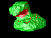 |
Fig. 1 SHAP5 shape model (Jorda et al. 2016) of comet 67P. Areas that are obscured in any common global map projection are colored red. |
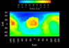 |
Fig. 2 SHAP5 shape model of 67P in equidistant cylindrical projection. The color encodes the distance from the comet center. A 3D view of the shape model is shown in Fig. 1. |
- 1.
randomly chose a 3D surface point r = (x, y, z) from theshape (here, we randomly picked a vertex of the shape model);
- 2.
find the map grid point (i, j) that holds the 3D position ri,j closest to the surface point (in 3D Euclidean distance ∥ri,j −r∥);
- 3.
tear the 3D position ri,j attached to the found grid point (i, j) toward the surface point r;
- 4.
also tear the 3D positions rk,l attached to grid points (k, l) in the vicinity of the found point toward the surface point r, but weighted with a factor that decreases with the distance from the found point, where the distance d is measured on the 2D map, that is, is computed from the horizontal and vertical indices of the grid point through
 . We used a Gaussian
  for the weighting factors.
Step 4 ensures the formation of a coherent map, that is, a map that preserves neighboring relationships of points on the real shape. However, the distance scale for the weighting of points in the vicinity has continuously to be turned down to a low value toward the end of the optimization in order to avoid the implied smoothing effect. We started with a 1σ reach of the Gaussian of 20% of the grid edge length and reduced it linearly to a reach of one grid step width at the end of the iteration. Similarly, the amount by which the found grid points are torn toward the presented surface point has to be continuously turned down in order to avoid noise created by the presentation of randomly selected surface points. Here, we started with tearing 10% of the distance to the presented point and, reducing the factor linearly as well, end with a factor of 10−6. The parameter starting values and their modification in the course of the iterations could be optimized to minimize the number of required iterations and thus the computation time. This was not done here. We reduced the parameter values rather slowly, which ensures the formation of a proper map, and accepted a large number (1–5 million) of iterations. In some cases, the map became entangled and did not unfold itself completely. Then the optimization had to be restarted from a different set of random positions.
Figure 3 shows a low-resolution toy model map consisting of 21 × 21 grid points fittedto the SHAP5 shape model of 67P. We use a low-resolution model here to make the individual quadrangular tiles of the shape model clearly visible. The grid wraps itself around the shape like a coat, trying to cover it as evenly as possible with all its grid points. The local density of map grid points tries to follow the frequency of the sample surface points presented tothe map during the learning process. Ideally, the sample points should be evenly distributed over the surface of the shape. This is not exactly the case here because we used the SHAP5 model vertices and the plate sizes vary to some extent. However, the vertices are fairly evenly distributed for the SHAP5 shape model. If a shape model with strongly varying plate sizes were used, this would have to be accounted for by presenting a randomly selected vertex point only with a probability that corrects for the local vertex density. In order to deal with an artifact, we have to introduce some bias into the sample point density in any case (Sect. 3.2).
We note a gap in Fig. 3 where the edges of the map approach each other. This gap becomes narrower with increasing grid resolution, but it never closes completely. In Sect. 3 we present an approach that completely avoids the gap. While this was at first the sole purpose of the approach we took, it turned out to have further benefits far beyond that. These are discussed in Sect. 4.
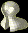 |
Fig. 3 Low-resolution toy model version with 21 × 21 grid points of a simple square Kohonen map fit to the comet surface. |
3 Creation of the QuACK map
3.1 Closing the grid
We created an inherently closed structure by taking two square grids and sewing them together at all four edges, see Fig. 4. Where two edges meet each other, only one is optimized during the learning procedure and is finally copied over to the other edge. First, we again used a toy version consisting of 41 × 21 grid points for the total of the two squares.
This closed map was then fit to the SHAP5 shape model of 67P in a similar way as the original open Kohonen map, see Sect. 2, again starting from low random values in the order of 0.001 km. The optimization procedure is illustrated in Fig. 5. The result is a complete map of the whole surface. The two squares can be unfolded into a rectangular map by breaking the seam at three of the four edges.
3.2 Artifact and its treatment
When the closed map is trained with the shape in exactly the same way as the original Kohonen map, a spurious ridge connecting head and body emerged in the neck area of the duck-like shape of 67P. This is shown for a low-resolution toy version with a grid size of 41 × 21 in Fig. 6. This artifact is persistently present in the closed map for different resolutions and different random starting positions.
The cause for the emergence of the ridge can be understood from the extremely concave shape in this part of the neck area. A point on top of the ridge is closer to the nearest head point at one end of the ridge or the nearest body point on the other end than to a neck point at the foundation of the ridge. Therefore, the ridge builds up and does not flatten out during the learning procedure. The simple open Kohonen map, see Sect. 2, seems to have more freedom in how to arrange itself around the shape and does not develop this artifact.
The solution that we finally found to this problem of the closed map is to present surface points below the ridge with twice the probability than other surface points during the learning process. If a randomly selected surface point was more than 1 km away from the comet center, it was only presented to the map with a 50% probability. The result of this modified learning procedure that completely suppresses the ridge is shown in Fig. 7. Giving higher weight to the surface points below the ridge yields a slightly higher density of map grid points in this area, but the grid point density varies in any case, particularly close to the four corner points.
3.3 Iterative optimization of the closed map
Apart from giving more weight to points in the lower neck area, see Sect. 3.2, the closed map was fit to the comet shape in thesame way as the classical Kohonen map, see Sect. 2. However, the closed nature seems to reduce the ability of the map to unfold completely, and we observe more cases where the map becomes entangled, here mostly in a twisted manner. We solved this in the same way as for the classical Kohonen map by restarting the optimization from a different set of random positions.
The full size map has a grid of 401 × 201 points. Usually, one million presentations of a surface point are by far sufficient to converge to the final solution, without any sophisticated optimization of the learning parameters and their evolution over the course of the iterations, see Sect. 2. For our final version, we iterated over five million presentations, which took several hours of computation time.
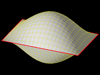 |
Fig. 4 Illustration of the creation of the closed map by sewing together two square grids at all four (red) edges. The shown 3D shape has no actual meaning, it only serves to illustrate the topology of the closed map. |
 |
Fig. 5 Illustration of the QuACK map learning procedure. The difference to the simple Kohonen map is that where two edges match at a seam, only one edge is optimized and its results are copied over to the other edge at the end. When the proximity of map grid points is assessed (cf. step 2 on the list in Sect. 2), the topology of the closed structure has to be taken into account. |
3.4 Resulting map
The QuACK map learns the shape from a model and is also a shape model in its own right, with relatively low resolution, but with the additional property that it can be unfolded to a rectangular grid. While we have so far used a low-resolution toy model of 41 × 21 grid points for illustration purposes, we now switch to our full-resolution map. The full-size QuACK shape model consisting of 401 × 201 grid points is shown in Fig. 8. Its 80 000 plates are quadrangles, not triangles as for other shape models of 67P. However, in order to apply software that only works on triangular meshes, each quadrangle can be cut into two triangles.
The special property of the QuACK shape model is that the vertices of the quadrangles are ordered along the lines of a two-dimensional grid, so that there is a unique relation between any point on the surface of the 3D shape model and a position on the map defined by the grid. The QuACK grid can be unfolded to a rectangular map with two squares side by side, where the left square approximately represents the northern hemisphere and the right square approximately represents the southern hemisphere, see Fig. 9. It is not coincidental that the two hemispheres arrange themselves in this way. It is rather caused by the fact that the rotation axis of the comet (which determines the location of the poles) is not random, but coincides with the principal axis of maximum moment of inertia. Thus, the equator area, which approximately runs around the edges of the map shown in Fig. 9, contains the regions with the largest distance from the comet center. The four corners of the two QuACK map squares go preferably to these distant regions and also to regions of large curvature. The corners go to the beak, the back head, the chest, and the tail of the duck-like shape of 67P. This is consistently reproduced from different sets of random starting positions.
This side-by-side layout is particularly useful to study hemispheric asymmetries. As an example, illumination maps are presented inSect. 6.
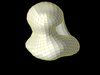 |
Fig. 6 Low-resolution toy version with 41 × 21 grid points of the QuACK map with a ridge-like artifact between head and body of the duck-like shape of 67P. |
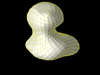 |
Fig. 7 Low-resolution toy version of the QuACK map in which the artifact between head and body shown in Fig. 6 is successfully suppressed. |
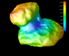 |
Fig. 8 QuACK shape model as it results from the learning procedure. It consists of 401 × 201 grid points. The color encodes (just as example data) the distance of the surface point from the comet center. |
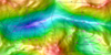 |
Fig. 9 Unfolded QuACK map of the color-encoded distance from the comet center. The 401 × 201 data points are the same as in Fig. 8. The two squares that were sewn together (cf. Fig. 4) are displayed side by side. The left square approximately represents the northern hemisphere, and the right square shows the southern hemisphere. Latitudes are depicted in black and longitudes in magenta. The low (bluish) area is the neck, above is the head, and below the body of the duck-like shape of 67P. |
3.5 Tessellation properties and map layout options
As illustrated in Fig. 10, the left and right edge of the unfolded rectangular map with two squares side by side match exactly. The top and bottom edges match if one map is rotated upside down. Thus, the landscape layout with the two hemispheresside by side can be transformed into a portrait layout, in which the two hemispheres lie one above the other, or into the square quincuncial layout, where the north pole is approximately in the center and the south pole approximately in the corners (or vice versa). Because it is constructed from two squares, it exhibits the same tessellation properties as the Peirce quincuncial projection of the world, which maps (in a first step) each hemisphere conformally to a square, see Sect. 4.1. These tessellation properties allow different map layouts, for example, in order to center a particular region of interest or for personal taste.
The map in quincuncial layout is shown in Fig. 11. It is elucidating to follow the zero meridian, which runs upward from the north pole close to the map center. It intersects the 30° latitude at three different points, which illustrates once more that we have different points with the same longitude and latitudein this area. In Fig. 12 the areas that are not visible in standard map projections are grayed out. The largest gray patch slightly above the north pole is a particularly interesting area, see Sect. 6.
Figure 13 shows another application of the QuACK map, again in quincuncial layout. This displays the different regions of the comet (region definitions according to Thomas et al. 2018).
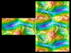 |
Fig. 10 Illustration of the tessellation properties of the QuACK map shown in Fig. 9 and the construction of the quincuncial layout. The square map in quincuncial layout consists of five parts: one center square approximately represents the northern hemisphere, and four right triangles that make up the southern hemisphere. |
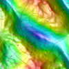 |
Fig. 11 QuACK map in quincuncial layout. It has been constructed from the side-by-side layout shown in Fig. 9 as illustrated in Fig. 10. |
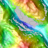 |
Fig. 12 Same as Fig. 11, but the areas that are not visible in standard map projection are overlaid in gray. These correspond to the areas shown in red in the shape model in Fig. 1. |
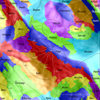 |
Fig. 13 Another application of the QuACK map in quincuncial layout, showing the different regions of 67P. Latitudes are depictedblack and longitudes in white. |
4 Generalized longitudes and latitudes
4.1 Peirce quincuncial projection of the world
The Peirce quincuncial projection of the world (Peirce 1879) is essentially a conformal (locally shape-preserving) projection that maps a hemisphere to a square. Thus, both hemispheres are mapped to two squares. The edges of each square represent the equator, thus the two squares are topologically connected in the same way as the two squares forming the QuACK map, see Sect. 3.5, in particular, Fig. 4. The Peirce quincuncial projection of the world is shown in Fig. 14. In the quincuncial layout invented by Peirce, the northern square is rotated by 45° to sit on a corner and the southern square is cut into four pieces that are attached to the edges of the northern square, forming a single square that displays the whole world. The construction of this layout is illustrated for the QuACK map in Fig. 10. Our QuACK map exhibits exactly the same tessellation properties (see Sect. 3.5) as the Peirce quincuncial projection. Therefore, the very same quincuncial layout can also be used for the QuACK map, see Figs. 11 and 13.
The conformity of the quincuncial projection is not fulfilled at four singular points, which are at the corners of each square. Toward these points, the area distortions become very strong. While the quincuncial projection does not preserve the area in any case, the distortions are small over most of the area. The zero meridian of the projection was chosen so that the critical points are in the oceans, away from the continents. Compared to other map projections, the distortions are therefore relatively small over the continents.
The fact that the South Pole is located at the corners of the map and that Antarctica is cut into four pieces could be considered ashortcoming of the map. We present an oblique version that overcomes this shortcoming and displays all continents, including Antarctica, without any intersection in Sect. 4.4.
4.2 Association of the QuACK map with the Peirce map
The QuACK projection has the same topology as the Peirce quincuncial projection of the world. It is a kind of generalized version of the quincuncial projection that breaks the degeneracy of multiple points for the same longitude and latitude for an irregular shape such as that of 67P.
We have seen in the QuACK map, for instance in Fig. 11, that longitudes and latitudes can have multiple intersections. This is the case for some extended areas shown gray in Fig. 12. Figure 14 shows longitudes and latitudes of the Peirce quincuncial projection of the world. They form a regular pattern, and there are of course no multiple intersections. The topological equivalence between Pierce projection and the QuACK projection makes it possible to define generalized longitudes and latitudes for 67P. To every point in the QuACK projection of 67P as shown in Fig. 11, we attach the longitude and latitude of the point with the same map location in the Peirce projection shown in Fig. 14. These generalized longitudes and latitudes are quite different from the original ones in the area where the latter are degenerated, but they are relatively similar over the rest of the comet. In particular, the north pole and the south pole in generalized longitude and latitude are close to the respective poles in original coordinates.
4.3 Arbitrary generalized projections
While the QuACK projection can be viewed as a generalized version of the Peirce quincuncial projection, the generalized longitudes and latitudes can be used to create a generalized version of any other projection by applying the respective projection to the generalized longitude and latitude. In this way, generalized versions of the cylindrical equidistant, the Mercator, the sinusoidal, the Mollweide, and any other projection can also be created. They all share the uniqueness of the longitude and latitude of the QuACK map projection.
In Fig. 15 we show for comparison the color-encoded distance of a point from the comet center in a standard equidistant cylindrical projection. Differently from Fig. 2, we only plot individual points that represent the vertices of the QuACK shape model. The overhung area where points with different distance from the comet center have similar longitude and latitudecan clearly be identified in the upper center of the map. The same data are shown in a generalized equidistant cylindrical projection in Fig. 16. We note that longitude and latitude no longer show ambiguities or discontinuities.
The generalized version of a projection will not exactly share any preservation properties of its original version. While the sinusoidal projection is exactly area preserving, the generalized version will only be approximately area preserving, for example. Similarly, the generalized version of the Mercator projection will only be approximately shape preserving (conformal), not exactly like its original. In particular for the quincuncial projection, which is conformaleverywhere with the exception of four singular points, the QuACK map, which can be seen as its generalized version, is nowhere exactly conformal. However, the QuACK map preserves area and shape relatively well over almost the complete surface of 67P and only exhibits significant distortions close to the four critical points.
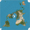 |
Fig. 14 Illustration of Peirce quincuncial projection of the world (Daniel R. Strebe, 23 July 2012, CC BY-SA 3.0). The red square represents the equator. |
4.4 Oblique projections
No global projection can be area preserving and shape preserving (conformal) at the same time everywhere. The grade of deficiency varies over the sphere. The equidistant cylindrical projection, for example, is perfectly area and shape preserving at the equator, with increasing distortion toward the poles.
For a particular application, it may be desirable to avoid projection deficiencies in certain areas of interest. This can be achieved by an oblique version of a map projection. An oblique version means that the sphere is rotated before the application of the projection, which shifts any deficiencies to a different area.
With the introduction of generalized longitude and latitude, we can also apply oblique versions of any generalized global projection to 67P. In particular, we can apply oblique versions of the QuACK map projection itself, which can be seen as a generalized version of the quincuncial projection, see Sect. 4.3.
As an example for the possible benefits of an oblique version of the quincuncial projection, we present an application to the Earth in Fig. 17. In the original version of the quincuncial projection, see Fig. 14, the four critical points toward which area distortions become strong are situated at the equator. For our oblique version, we first rotated the sphere by 45° counterclockwise around the y-axis (z is the comet rotation axis, the x-axis goes through the zero meridian). This moved the point with original longitude 0° and latitude 45° to the North Pole. Then we rotated the sphere by 45° counterclockwise around the z-axis. This moved the zero meridian to longitude − 45°. As a consequence of these operations, the four critical points are located in the oceans, away from the continents, similarly to the original quincuncial projection, and moreover, Antarctica is moved away from the center of the southern square.
The quincuncial projection maps each hemisphere (as newly defined after the above rotations) to a square. We chose another special layout with the northern square centered (but not rotated to sit in a corner, as in the quincuncial layout) and the southern square vertically cut into half, one half displayed to the left of the center square and the other to the right. Reflecting the naming of the quincuncial projection, we call this the triptychial projection of the world. With this layout, we can show all continents, including Antarctica, without any intersections. The four critical points are located at the corners of the center square at the top and the bottom edge of the map. Because they are situated in the oceans, the distortion is small over the continents. Close to the top left critical point located at the top edge half-way between the center and the left corner, we note the Galapagos islands, which are considerably distorted and displayed too large because they are close to the critical point. If desired, this could be avoided by some fine-tuning of rotation angles and map layout. Similarly, the generalized longitudes and latitudes defined with the QuACK map make it possible for 67P to shift the particular deficiencies of any map projection away from areas of interest.
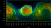 |
Fig. 15 Distance of a point from the comet center in equidistant cylindrical projection. The color scale is the same as in Fig. 2. Each point represents a vertex of the QuACK shape model, a 3D view of which is shown in Fig. 8. |
5 Implementation of the QuACK map projection
5.1 shapeViewer software
The QuACK map projection is implemented into the shapeViewer software by Jean-Baptiste Vincent1.
5.2 Subroutines to facilitate the projection
We make a collection of subroutines and data to facilitate the QuACK map projection available at GitHub2. So far, this includes the QuACK shape model in VER format in quadrangle plate and triplate version and a SPICE digital shape kernel (DSK). Subroutines are available to transform a 3D position on the surface of the QuACK shape model to QuACK map coordinates in hemisphere side-by-side layout and to transform these into quincuncial layout and also into generalized longitudes and latitudes.
 |
Fig. 17 Oblique version of the quincuncial projection for the Earth. As our layout consists of three parts (see text), we call it the triptychial projection of the world. It shows all continents, including Antarctica, without any intersections and with only small distortions. The underlying surface data are the Envisat mosaic from May–November 2004 (ESA, 3 May 2005, CC BY-SA 3.0 IGO). |
5.3 Using the special QuACK shape model
The application of the projection given by the QuACK map is more complicated than applying any of the standard global projections given by an analytic expression. The relation between 3D shape and 2D map is instead defined by a shape model with special properties.
In order to apply the QuACK map, when projecting data onto the surface of 67P, for instance, imagery, it is preferable to work directly with the QuACK shape model. For every shape model vertex, the map coordinates are directly known. If the accuracy of the 401 × 201 grid is sufficient, the nearest vertex can therefore be picked.
If subgrid accuracy is desired, the position within a plate has to be interpolated. Subroutines facilitating bilinear interpolation are available, see Sect. 5.2. In this way, although the QuACK shape model has a relatively low resolution, data with arbitrary high resolution can consistently be projected onto the QuACK map.
5.4 Transforming between different shape models
If the data are not defined directly on the QuACK shape model, for example, if they have been projected onto another shape model and repeating the projection with the QuACK shape model is not desired, the situation is slightly more complicated (and consumes more computation time).
If the resolution of the QuACK map grid is sufficient, the closest vertices (or plate centers) of the two shape models can be associated with each other. This is very simple to apply but may consume very much computation time if the other shape model has a very high resolution. This method was used to transform the comet region definitions shown in Fig. 13 from the very high-resolution SHAP7 shape model (Preusker et al. 2017) on which they were provided (Thomas et al. 2018) into the QuACK shape model. The individual QuACK map grid pixels can be identified upon close inspection.
A standard method to achieve the transformation with subgrid accuracy would be interpolation based on weighted nearest neighbors. For an arbitrary 3D point, the Euclidean distances to its nearest neighbors in the QuACK shape are computed. This can usually be limited to a certain number of nearest neighbors or to a certain radius. From these distances, weights are determined, usually by just applying a negative exponent, typically − 1. The weighted sum of the respective points of the QuACK map gives the searched-for 2D map position. For most applications, this standard method may provide acceptable results, but in principle, distortions on subgrid level may be introduced.
The accurate projection of high-resolution data given in one shape model onto another shape model without introducing distortions in the interior of plates and discontinuities at the edges is by no means trivial. In particular, a unique solution may not exist.
The best solution might be considered as a QuACK shape model with the same resolution as the highest resolution shape models available. However, on one hand, this is computationally prohibitive, and on the other hand, the higher the resolution and the more irregular the shape, the more difficult the unambiguous transformation of data from another shape model. In this respect, we recommend to rather follow the approach described in Sect. 5.3.
6 Example application: illumination maps
Various scientific investigations of a solar system body are facilitated by the availability of complete global maps. An example particularly applicable to an irregularly shaped comet are illumination maps. These allow studying the relation between incoming insolation and observed surface temperature or comet activity, for example.
The daily mean illumination of any surface point varies with season. Making use of the Rosetta SPICE kernel data set (Vazquez-Garcia et al. 2017), we have computed the illumination for all tiles of the QuACK shape model (cf. Fig. 8) by averaging over one full solar day with a time step of one minute, taking into account the surface normal of the tile and self-shadowing by other terrain. This was conducted for two epochs, first the time of arrival of Rosetta at 67P on 8 August 2014, which is close to summer solstice, and second at perihelion on 13 August 2015, which is close to winter solstice.
In order to study the asymmetry of the potential erosion due to solar insolation between the cometary summer and winter seasons, the side-by-side layout shown in Fig. 9 is particularly useful. Illumination maps in the very same layout of the QuACK map projection for both epochs are presented in Fig. 18. Because of the different distances from the Sun at the two epochs, there is an order of magnitude difference in the illumination value, and hence different color scales are used.
The map layout enables a direct comparison of the two hemispheres. Each polar night zone can be examined as one coherent area. Similarly, the complete neck area is coherently visible. It runs from left to right, edge to edge, see Fig. 9, and can also be extended on either edge because of the tessellation properties, see Fig. 10. The overhung northern neck area is particularly interesting. It is visible for both epochs as a cyan tongue entering from the left edge in the upper part. It is darker than most of the northern hemisphere in summer, but brighter in winter. Remarkably, this area receives an order of magnitude more illumination in winter than in summer. This very important area would be invisible in standard global projection, see Fig. 12.
Any remote-sensing data of any area on the surface can be displayed in the same map projection and thus directly be compared tothe illumination. This would help to promote the understanding of the relationships between illumination and comet activity.
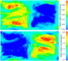 |
Fig. 18 Daily mean illumination of 67P (in units of the irradiance received by a point at Earth’s equator, averaged over one rotation, for a distance of 1 AU from the Sun) in the side-by-side layout of the QuACK map projection. The norther hemisphere is to the left and the southern hemisphere to the right. For the relation to the topography of 67P and longitudes and latitudes, see Fig. 9. Top: arrival time of Rosetta at 67P, 8 August 2014, close to summer solstice. Bottom: perihelion, 13 August 2015, close to winter solstice. |
7 Summary and discussion
We have extended the algorithm of the self-organizing Kohonen map to the quincuncial adaptive closed Kohonen (QuACK) map. The QuACK map allows displaying the complete surface of 67P in a global map (Figs. 11 and 13), including the overhung areas where multiple points exist for the same longitude and latitude. These points are invisible in standard map projections (Figs. 1 and 12). An example for the application of the QuACK map projection are illumination maps (Fig. 18).
The QuACK map is topologically equivalent to the Peirce quincuncial projection of the world (Fig. 14). Similarly, it preserves area relatively well over most of the map. It differs in that it is not exactly (but still approximately) shape preserving (conformal). The relation with the Peirce quincuncial projection allows us to define generalized longitudes and latitudes on the QuACK map, which are unique over the complete map. These enable generalized versions of any standard global projection (and also oblique versions of these) that also display the complete comet (Fig. 16).
A QuACK map can be fit to any irregular shape. However, this only makes sense if the shape comprises overhung areas that would be invisible in standard map projections, or at least high slopes that would cause considerable distortions. Otherwise, the QuACK map would be very similar to the quincuncial projection.
The application of the QuACK map projection is more complicated than the application of a standard map projection given by an analytic formula. The QuACK map is defined by a special shape model that can be unfolded to a rectangular map (Figs. 8 and 9). The use of the QuACK map is facilitated by working directly with the QuACK shape model.
As a byproduct of our investigations and as an example for a useful oblique version of the Peirce quincuncial projection, we presented the triptychial projection of the world, which is shape preserving (conformal) and exhibits only small distortions over the continents, like the quincuncial projection. However, it has the advantage that it displays all continents, including Antarctica, without anyintersection (Fig. 17).
References
- Jorda, L., Gaskell, R., Capanna, C., et al. 2016, Icarus, 277, 257 [NASA ADS] [CrossRef] [Google Scholar]
- Kohonen, T. 1982, Biol. Cybern., 43, 59 [Google Scholar]
- Peirce, C. S. 1879, Am. J. Math., 2, 394 [CrossRef] [Google Scholar]
- Preusker, F., Scholten, F., Matz, K. D., et al. 2015, A&A, 583, A33 [NASA ADS] [CrossRef] [EDP Sciences] [Google Scholar]
- Preusker, F., Scholten, F., Matz, K.-D., et al. 2017, A&A, 607, L1 [NASA ADS] [CrossRef] [EDP Sciences] [Google Scholar]
- Thomas, N., El Maarry, M. R., Theologou, P., et al. 2018, Planet. Space Sci., 164, 19 [NASA ADS] [CrossRef] [Google Scholar]
- Vazquez-Garcia, J. L., Zender, J., Barthelemy, M., Semenov, B., & Costa, M. 2017, ROSETTA ORBITER/LANDER SPICE KERNELS V1.0, RO/RL-E/M/A/C-SPICE-6-V1.0 [Google Scholar]
All Figures
|
Fig. 1 SHAP5 shape model (Jorda et al. 2016) of comet 67P. Areas that are obscured in any common global map projection are colored red. |
| In the text | |
|
Fig. 2 SHAP5 shape model of 67P in equidistant cylindrical projection. The color encodes the distance from the comet center. A 3D view of the shape model is shown in Fig. 1. |
| In the text | |
|
Fig. 3 Low-resolution toy model version with 21 × 21 grid points of a simple square Kohonen map fit to the comet surface. |
| In the text | |
|
Fig. 4 Illustration of the creation of the closed map by sewing together two square grids at all four (red) edges. The shown 3D shape has no actual meaning, it only serves to illustrate the topology of the closed map. |
| In the text | |
|
Fig. 5 Illustration of the QuACK map learning procedure. The difference to the simple Kohonen map is that where two edges match at a seam, only one edge is optimized and its results are copied over to the other edge at the end. When the proximity of map grid points is assessed (cf. step 2 on the list in Sect. 2), the topology of the closed structure has to be taken into account. |
| In the text | |
|
Fig. 6 Low-resolution toy version with 41 × 21 grid points of the QuACK map with a ridge-like artifact between head and body of the duck-like shape of 67P. |
| In the text | |
|
Fig. 7 Low-resolution toy version of the QuACK map in which the artifact between head and body shown in Fig. 6 is successfully suppressed. |
| In the text | |
|
Fig. 8 QuACK shape model as it results from the learning procedure. It consists of 401 × 201 grid points. The color encodes (just as example data) the distance of the surface point from the comet center. |
| In the text | |
|
Fig. 9 Unfolded QuACK map of the color-encoded distance from the comet center. The 401 × 201 data points are the same as in Fig. 8. The two squares that were sewn together (cf. Fig. 4) are displayed side by side. The left square approximately represents the northern hemisphere, and the right square shows the southern hemisphere. Latitudes are depicted in black and longitudes in magenta. The low (bluish) area is the neck, above is the head, and below the body of the duck-like shape of 67P. |
| In the text | |
|
Fig. 10 Illustration of the tessellation properties of the QuACK map shown in Fig. 9 and the construction of the quincuncial layout. The square map in quincuncial layout consists of five parts: one center square approximately represents the northern hemisphere, and four right triangles that make up the southern hemisphere. |
| In the text | |
|
Fig. 11 QuACK map in quincuncial layout. It has been constructed from the side-by-side layout shown in Fig. 9 as illustrated in Fig. 10. |
| In the text | |
|
Fig. 12 Same as Fig. 11, but the areas that are not visible in standard map projection are overlaid in gray. These correspond to the areas shown in red in the shape model in Fig. 1. |
| In the text | |
|
Fig. 13 Another application of the QuACK map in quincuncial layout, showing the different regions of 67P. Latitudes are depictedblack and longitudes in white. |
| In the text | |
|
Fig. 14 Illustration of Peirce quincuncial projection of the world (Daniel R. Strebe, 23 July 2012, CC BY-SA 3.0). The red square represents the equator. |
| In the text | |
|
Fig. 15 Distance of a point from the comet center in equidistant cylindrical projection. The color scale is the same as in Fig. 2. Each point represents a vertex of the QuACK shape model, a 3D view of which is shown in Fig. 8. |
| In the text | |
 |
Fig. 16 Same data as in Fig. 15 in generalized equidistant cylindrical projection. |
| In the text | |
|
Fig. 17 Oblique version of the quincuncial projection for the Earth. As our layout consists of three parts (see text), we call it the triptychial projection of the world. It shows all continents, including Antarctica, without any intersections and with only small distortions. The underlying surface data are the Envisat mosaic from May–November 2004 (ESA, 3 May 2005, CC BY-SA 3.0 IGO). |
| In the text | |
|
Fig. 18 Daily mean illumination of 67P (in units of the irradiance received by a point at Earth’s equator, averaged over one rotation, for a distance of 1 AU from the Sun) in the side-by-side layout of the QuACK map projection. The norther hemisphere is to the left and the southern hemisphere to the right. For the relation to the topography of 67P and longitudes and latitudes, see Fig. 9. Top: arrival time of Rosetta at 67P, 8 August 2014, close to summer solstice. Bottom: perihelion, 13 August 2015, close to winter solstice. |
| In the text | |
Current usage metrics show cumulative count of Article Views (full-text article views including HTML views, PDF and ePub downloads, according to the available data) and Abstracts Views on Vision4Press platform.
Data correspond to usage on the plateform after 2015. The current usage metrics is available 48-96 hours after online publication and is updated daily on week days.
Initial download of the metrics may take a while.