| Issue |
A&A
Volume 630, October 2019
Rosetta mission full comet phase results
|
|
|---|---|---|
| Article Number | A33 | |
| Number of page(s) | 14 | |
| Section | Planets and planetary systems | |
| DOI | https://doi.org/10.1051/0004-6361/201834226 | |
| Published online | 20 September 2019 | |
Two years with comet 67P/Churyumov-Gerasimenko: H2O, CO2, and CO as seen by the ROSINA/RTOF instrument of Rosetta
1
IRAP, Université de Toulouse, CNRS, UPS, CNES, Toulouse, France
e-mail: margaux.hoang@irap.omp.eu
2
University of Bern, Physics Institute, Bern, Switzerland
3
Department of Physics, Imperial College London, London, UK
4
Technical University of Braunschweig, Braunschweig, Germany
5
Max-Planck Institute for Solar System Research, Göttingen, Germany
6
Southwest Research Institute, San Antonio, TX, USA
Received:
12
September
2018
Accepted:
29
March
2019
Context. The ESA Rosetta mission investigated the environment of comet 67P/Churyumov-Gerasimenko (hereafter 67P) from August 2014 to September 2016. One of the experiments on board the spacecraft, the Rosetta Orbiter Spectrometer for Ion and Neutral Analysis (ROSINA) included a COmet Pressure Sensor (COPS) and two mass spectrometers to analyze the composition of neutrals and ions, the Reflectron-type Time-Of-Flight mass spectrometer (RTOF), and the Double Focusing Mass Spectrometer (DFMS).
Aims. RTOF species detections cover the whole mission. This allows us to study the seasonal evolution of the main volatiles (H2O, CO2, and CO) and their spatial distributions.
Methods. We studied the RTOF dataset during the two-year long comet escort phase focusing on the study of H2O, CO2, and CO. We also present the detection by RTOF of O2, the fourth main volatile recorded in the coma of 67P. This work includes the calibration of spectra and the analysis of the signature of the four volatiles. We present the analysis of the dynamics of the main volatiles and visualize the distribution by projecting our results onto the surface of the nucleus. The temporal and spatial heterogeneities of H2O, CO2, and CO are studied over the two years of mission, but the O2 is only studied over a two-month period.
Results. The global outgassing evolution follows the expected asymmetry with respect to perihelion. The CO/CO2 ratio is not constant through the mission, even though both species appear to originate from the same regions of the nucleus. The outgassing of CO2 and CO was more pronounced in the southern than in the northern hemisphere, except for the time from August to October 2014. We provide a new and independent estimate of the relative abundance of O2.
Conclusions. We show evidence of a change in molecular ratios throughout the mission. We observe a clear north-south dichotomy in the coma composition, suggesting a composition dichotomy between the outgassing layers of the two hemispheres. Our work indicates that CO2 and CO are located on the surface of the southern hemisphere as a result of the strong erosion during the previous perihelion. We also report a cyclic occurrence of CO and CO2 detections in the northern hemisphere. We discuss two scenarios: devolatilization of transported wet dust grains from south to north, and different stratigraphy for the upper layers of the cometary nucleus between the two hemispheres.
Key words: comets: individual: 67/Churyumov-Gerasimenko / comets: general / planets and satellites: atmospheres
© M. Hoang et al. 2019
 Open Access article, published by EDP Sciences, under the terms of the Creative Commons Attribution License (http://creativecommons.org/licenses/by/4.0), which permits unrestricted use, distribution, and reproduction in any medium, provided the original work is properly cited.
1 Introduction
The ESA Rosetta mission became the first spacecraft that followed a comet along its path around the Sun, and it was the first mission to achieve two landings on a comet. In addition to these technical advances, the 11 instruments on board Rosetta collected data during more than two years. The Rosetta spacecraft arrived at 67P/Churyumov-Gerasimenko (67P) for the rendezvous in August 2014, at about 3.6 au from the Sun. The mission ended with the landing of the spacecraft on the surface of the comet on 30 September 2016. The unprecedented amount of data gathered by Rosetta considerably increases our understanding of comets (Taylor et al. 2017).
The first resolved image of 67P taken by the Optical, Spectroscopic, and Infrared Remote Imaging System (OSIRIS) camera showed a bilobed body: a small lobe with a diameter of about 2 km and a large lobe of about 4 km, which are linked by an area called “the neck” (Sierks et al. 2015). The body has a rotation period of around 12.4 h, which changed to 12.0 h in 2016 (Accomazzo et al. 2017), and a rotation axis tilted by 52° (Jorda et al. 2016). Massironi et al. (2015) identified incompatible strata envelopes on the small and large lobes, suggesting that the bilobed shape is the result of a smooth collision between two independent bodies. The camera revealed a rugged surface of the illuminated side of the nucleus (northern hemisphere and equator at the beginning of the mission) with significant expanses of a smooth material, as described in Sierks et al. (2015). After the inbound equinox, the southern hemisphere came out of the shadow to reveal a surface with steeper topography (El-Maarry et al. 2016). Because of its high obliquity and its shape, the nucleus of 67P is subject to strong illumination variations. The Rosetta mission observed the seasonal evolution of the coma composition of 67P, in particular, the changes occurring during the equinoxes and perihelion passage.
Capaccioni et al. (2015) described a surface covered by a dark material, with a very low reflectance spectrum and no detectable ice patches in the northern hemisphere. Water-ice patches were later found on the surface (in diverse regions below a latitude of 30°) by Pommerol et al. (2015), De Sanctis et al. (2015), and Barucci et al. (2016) in observations made with the OSIRIS and Visible InfraRed Thermal Imaging Spectrometer (VIRTIS), showing a localized diurnal activity pattern after which water condensates on the surface. Although tens of water-ice spots have been observed, only a single spot of carbon dioxide ice has been identified on the surface, in the southern hemisphere (Anhur region) (Filacchione et al. 2016).
The spatial distributions of water and carbon dioxide have been investigated by Bockelée-Morvan et al. (2015), Migliorini et al. (2016), and Fink et al. (2016) using VIRTIS data from 24 November 2014 to 24 January 2015, from 8 to 14 April 2015, and from 28 February to 27 April 2015, respectively. Bockelée-Morvan et al. (2015) described a water production originating from the illuminated parts on the surface, in particular above the neck. They suggested that CO2 sublimates below the diurnal skin depth because CO2 has been detected in illuminated and non-illuminated regions. Migliorini et al. (2016) described two active water regions, Aten-Babi and Seth-Hapi, and high abundances of CO2 outgassing from the head and the southern hemisphere. Fink et al. (2016) confirmed the detection of H2O and CO2 outgassing from distinct origins. They proposed that the northern surface is depleted in CO2 and that the southern hemisphere is more pristine, and they observed that the concentration of CO2 arose from local spots in the southern hemisphere.
The Rosetta Orbiter Spectrometer for Ion and neutral analysis (ROSINA) experiment analyzed the composition of the coma of 67P with two spectrometers, the Double Focusing Mass Spectrometer (DFMS) and the Reflectron-type Time-Of-Flight (RTOF), and the sensor called Comet Pressure Sensor (COPS) (Balsiger et al. 2007). The coma composition varied strongly throughout the mission in terms of the dynamics of the main volatiles (H2O, CO2, and CO) and their ratios. Hässig et al. (2015) described the behavior of the three main volatiles seen by ROSINA/DFMS at the beginning of the mission, between August and September 2014, with a high CO2 /H2O ratio located on the southern side of the large lobe. Measurements from the pre-perihelion period revealed that H2O sublimation was correlated with the large illuminated areas of the surface, including the active neck region before equinox (10 May 2015) and moving slowly southward afterward. CO2 and CO outgassing were in general lower than H2O outgassing and were mostly confined to the southern hemisphere (Hoang et al. 2017). The non-detection of CO2 from the northern hemisphere during several months before the May 2015 equinox, even though surface temperatures were well above the sublimation temperature of CO2, suggests that an insulating layer of dust/water was transported from the southern hemisphere (Keller et al. 2017). Gasc et al. (2017a) also showed possible correlations between minor species (NH3, H2 S, CH4, and HCN) and the sublimation of pure ices mainly made of water and CO2 at about the second equinox in March 2016.
Le Roy et al. (2015) presented a chemical inventory of the molecules found in the coma at 3.15 au inbound and heterogeneities linked to the minor species. Moreover, Bieler et al. (2015) revealed the detection of molecular oxygen in large abundances in the coma, suggesting that O2 was trappedin the ice since the formation of the nucleus.
Hansen et al. (2016) compared the water production measured by DFMS, the Microwave Instrument for the Rosetta Orbiter (MIRO), VIRTIS and the Rosetta Plasma Consortium: Ion Composition Analyzer (RPC-ICA) for the whole mission. The maximum outgassing as seen with DFMS occurred 18 to 22 days after perihelion with a water production rate of 3.5 ± 0.5 × 1028 molecules s−1.
In this work, we present a study of the global outgassing of 67P seen by the RTOF mass spectrometer. We include results from Hoang et al. (2017; hereafter referred to as Paper I) to observe the evolution through the two years of mission. We analyze the entire dataset recorded by the instrument from September 2014 until the end of the escort phase in September 2016.
2 Method
2.1 Description of the instruments
The RTOF mass spectrometer was designed to measure cometary neutral gas and ions, and achieved a mass resolution of m∕Δm = 500 at 50% level because of a high-voltage problem. This time-of-flight spectrometer was able to detect ions and molecules from 1 to 300 u e−1 and had a high temporal resolution of 200 s (Scherer et al. 2006; Balsiger et al. 2007).
The RTOF spectrometer could be operated in two different configurations using two distinct channels: the storage source (SS), which samples the neutral gas, and the orthogonal source (OS), which analyzes cometary ions as well as neutral gas. Each ion source had two tungsten filaments that provided the electrons to ionize neutral particles by electron impact. Considering the limitations of the data rate and the compression of DPU data, both channels were never used at the same time in space.
The charged particles were extracted toward the drift tube by an extraction grid, applying a pull pulse at a frequency of 2, 5, or 10 kHz. The ions passed through the 83 cm long drift tube, were deviated back by the reflectron located at the end of the tube, and finally reached the detector. The time-of-flight spectrometer was able to recognize the nature of an ion through its speed in the drift tube because the time of flight of each molecule is proportional to the square root of the mass of the species.
The performance of the two mass spectrometers RTOF and DFMS was complementary. While RTOF had a high temporal resolution (200 or 400 s depending on the mode), DFMS possessed a high mass resolution of m∕Δm = 3000 at 1% level with a mass range of 12–150 u e−1. It scanned one mass range at a time, covering the full range from 13 u e−1 to more than 130 u e−1 in about 40 min (depending on the mode).
We used the COPS nude gauge (NG), which measured the in situ total ambient neutral number density. Unlike RTOF and DFMS, COPS was not able to distinguish the different species.
2.2 Dataanalysis
The number densities of the volatiles were derived from the RTOF spectra recorded in both channels using the SS and the OS. The first step of the data analysis was converting the spectra into physical units (i.e. u e−1). A mass calibration was applied to all spectra through the gas calibration unit mode (GCU mode) (Gasc et al. 2017b). The unit contained a well-defined mixture of helium, carbon dioxide, and krypton, covering a wide mass range. This mixture allowed us to convert the time-of-flight spectra into mass/charge (u e−1).
The second step was integrating the peaks corresponding to water (mass 18.01 u e−1), carbon monoxide (mass 27.99 u e−1), and carbon dioxide (mass 43.98 u e−1). The integration yielded the numerical area below the curve, which represents the number of ions per 200 or 400 s time bins depending on the operating mode. After we obtained the ion abundance of the three volatiles in each spectra, corrections due to specific sensitivity and fragmentation pattern of each species were applied. Finally, we were able to define the corresponding densities of the three studied molecules throughout the mission, after normalization to the measured COPS densities. Details of the data analysis applied to RTOF are given in Paper I and Gasc et al. (2017b). We note that further processing was applied to RTOF spectra since Paper I. They led to more accurate values for the density of the detected species.
3 Results
We present the number densities of the three main volatiles as recorded by RTOF from September 2014 until September 2016 in Fig. 1. We also show associated orbital parameters, such as the latitude of the sub-spacecraft (SSC) point, the cometocentric distance, and the heliocentric distance throughout the mission. The plotted densities are scaled to a distance of 1 km from the center of the nucleus assuming a 1/r2 dependence for comparison.
The dataset starts during the inbound part of the cometary orbit around the Sun, at a cometocentric distance of about 50 km. Rosetta remained around the nucleus during the outbound part up to a heliocentric distance of 3.88 au. The full mission dataset shows the evolution of the outgassing of the nucleus during the escort phase as a function of the heliocentric distance. The upper panel shows that RTOF did not continuously record data during the mission. Data were missed because of several reasons. Finally, data gaps appeared when the signal was below the detection limit of the instrument as a result of large comet-spacecraft distances (excursion of September 2015) or off-pointing of the spacecraft.
In the RTOF dataset, we distinguish seven periods of time to study the evolution of the coma through the mission, referred to in the text as periods A to G, as described in Table 1. A detailed study of the temporal and spatial variations of the three main volatiles during periods A, B, and E was given in Paper I, where they were called periods A, B, and C. We now describe the global evolution of the three main volatiles and their relative ratios CO2 /H2O and CO/H2O, as well as their spatial heterogeneities during the Rosetta mission. We then present an estimate of the relative abundance of O2 and its spatial distribution during period A.
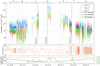 |
Fig. 1 Upper panel: temporal evolution of H2O, CO2, and CO densities multiplied by the cometocentric distance squared, derived from RTOF relative abundances scaled to COPS over the Rosetta mission. Colored lines are averaged over two comet rotations. Middle panel: latitude of the sub-spacecraft point in the 67P fixed frame. Lower panel: variation in distance between Rosetta and 67P (black) and the heliocentric distance (yellow). First equinox occurred on 2015 May 10 at 1.67 au, perihelion on 2015 August 13 at 1.24 au, andsecond equinox on 2016 March 21 at 2.63 au. RTOF data are missing during excursions of the spacecraft. Periods A to G are indicated above the first panel. They are described in Table 1. |
Description of the seven periods covering the RTOF dataset, with the corresponding heliocentric distances and the average subsolar latitudes.
3.1 Global temporal evolution
In Fig. 1 we show the datasets of the densities of H2O (in blue), CO2 (in red), and CO (in green), scaled to a distance of 1 km. We also show the data averaged over two rotations of the comet (colored lines) to filter the diurnal variations, highlighting the link between the temporal variation of densities and the SSC latitude, which we study in detail in Fig. 2. The number densities of the three volatiles, scaled to 1 km, are reportedin terms of lower quartile (Q1), median (Q2), and upper quartile (Q3) in Table 2.
The global evolution of the number densities of the main volatiles shows the expected increase in outgassing during the pre-perihelion period and decrease after perihelion, see Fig. 1 and Table 2. When the comet approached the Sun, the heating of the nucleus caused an increase in the ice sublimation. Around perihelion, the nucleus heating reached its maximum intensity. An asymmetry in the outgassing appears in the dataset, and we observe that the maximum sublimation occurs slightly after perihelion. About 10 to 15 days after perihelion, we estimate H2O number densities of 1.65 × 1012 cm−3 km2, CO2 number densities of 1.5 × 1011 cm−3 km2, and a CO reached 2.35 × 1011 cm−3 km2 at 1 km. This delay may be due to a combination of two effects: the proximity to the Sun, and the maximum illumination of the southern hemisphere (the illuminated hemisphere at that time), which occurred around the solstice, three weeks after perihelion. As described by Hansen et al. (2016), in period A, we observed an unexpected decrease in H2O while the heliocentric distance decreased. The CO and CO2 number densities follow the same trend. This observation was correlated with the motion of the spacecraft from the sunward side to the terminator.
Water was the main contributor to the gas composition of the coma, except during the last months of the mission. The contributionof carbon monoxide and carbon dioxide became more important during the last months. The behavior of CO/H2O and CO2/H2O ratios, derived from RTOF spectra, is detailed in Fig. 2. The lower quartile (Q1), median (Q2), and upper quartile (Q3) of CO2/H2O and CO/H2O for the seven periods are reported in Table 3. During period A, the ratio variations are synchronized, but the CO/H2O decreases while the CO2/H2O ratio increases slowly, and both reach similar values in October 2014. We then observed large variations for both ratios, with higher density values for CO2 (0.19 for CO2/H2O compared to0.09 for CO/H2O in period B). In the intermediate dataset of 2015 (periods C and D), the CO/H2O ratio is the highest. After the outbound equinox, the ratios of CO2 and CO versus H2O globally increased, both temporarily exceeded 5 and CO2/H2O even reached 25 in September 2016. From average number density ratios of 0.03 for CO2/H2O and 0.08 for CO/H2O during period C, the values increased to 0.57 and 0.36, respectively, for period G.
The SSC latitude is shown in the lower panel and the correlation with the ratios variation can be studied. Before the first equinox and after the second equinox, the high number density ratios are mainly located in the southern hemisphere, confirming the strong hemispherical asymmetry of CO and CO2 during the mission. The variations in the ratios are mainly due to the variations in the water density in the coma. Nevertheless, we observed larger variations in the CO2/H2O ratio than inCO/H2O, suggesting that the heterogeneity of CO2 is stronger.
Details of the temporal variabilities and changes in outgassing for September 2014 to February 2015 and for December 2015 to February 2016 are given in Hoang et al. (2017); for the 2016 March equinox, they are listed in Gasc et al. (2017a). The paucity of RTOF data during the six months after perihelion makes interpretating these data more difficult during this period. Specific periods of densities evolution are discussed below in Fig. 3 (after the 2016 March equinox) and Fig. 4 (end of December 2016).
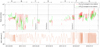 |
Fig. 2 Upper panel: time evolution of CO/H2O and CO2 /H2O density ratios for the entire mission, starting in September 2014 and ending in September 2016. Lower panel: variation in SSC point latitude in degrees. Periods A to G are indicated above the first panel, and they are described in Table 1. |
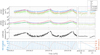 |
Fig. 3 Left: temporal evolution after equinox of the densities of the RTOF (first panel) and DFMS main volatiles (second panel) with the average over two comet rotations (colored lines), the COPS nude gauge total densities (third panel), and the SSC point latitude and longitude (fourth panel). Right: zoom-in on one rotation (~12 h). |
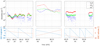 |
Fig. 4 Number densities of the main volatiles for the five last days of RTOF measurements (upper panels) and corresponding SSC latitude and longitude (lower panels). |
3.1.1 Post-equinox
Figure 3 presents the detailed data recorded at the end of June 2016 and beginning of July 2016, after the second equinox (left), with a zoom-in on one rotation of 12 h (right). At that time, the subsolar latitude moved from the southern to the northern hemisphere. The first panel of Fig. 3 shows the densities of the RTOF main volatiles and the second panel shows the corresponding DFMS data. The variations in COPS pressures are shown in the third panel. They are total gas densities because COPS cannot distinguish the different volatiles. The corresponding SSC latitude (lower panel) indicates that the ice sublimation mostly occurs in the southern hemisphere. The increase in temperature of the nucleus surface is the result of previous illumination of the southern hemisphere, while the heating in the northern hemisphere is not yet sufficient to cause large sublimation of volatiles (Keller et al. 2015). The lower panel also indicates the SSC longitude. The quick variations in coma densities are linked to the non-spherical shape of thecomet (Hässig et al. 2015) because the surface of the illuminated nucleus that is visible in the field of viewof RTOF changes with the rotation of the nucleus. Except when the SSC latitudes are lower than −45°, the water appears to exceed CO2 and CO in the coma composition.
The excellent temporal resolution of RTOF is visible in the upper panel of Fig. 3, with a measurement every 200 s. This gives us the detailed temporal dynamics of the coma composition. At that time, the three volatiles were strongly correlated, suggesting very similar source emission regions. In the second panel of Fig. 3, the DFMS densities forthe three volatiles are given for the same time. To do so, the derived densities were time-interpolated and time-shifted to the time of the water measurements, that is, about 40 min, as shown in the right panel. The comparison between the two instruments (see Paper I) reveals that they are globally in good agreement with each other. Nevertheless, as observed in this example, the datasets are not identical, and clear differences appears. The water outgassing is underestimated by DFMS, it appears lower than in the RTOF panel. In particular, the CO2 detections are overestimated around the maximum, and the CO detections are slightly overestimated. RTOF and DFMS are two distinct instruments, located at two different positions on the spacecraft and with different mass and time resolutions, which induces a more important diffusion in the RTOF measurements and explains that the two datasets present differences. Furthermore, both datasets are obtained after much processing during the conversion of abundance into densities. It is hard to tell which instrument estimates the volatile dynamics best.
3.1.2 End of mission
The instrument was turned on sporadically during the last two months of the mission, based on available power. In Fig. 4 we present a zoom of the very last detections of the main volatiles seen by RTOF, on 21, 23, and 25–26 September 2016. At that time, 67P was at 3.83 au from the Sun. As a result of approach maneuvers, the cometocentric distance of Rosetta varied between 4 and 17 km during September 2016.
We observe the different behaviors of the three main volatiles at close distances from the nucleus. During 2016, water abundances slowly decreased as the comet moved away from the Sun. At the end of the mission, water number densities were mainly below the values of carbon dioxide and carbon monoxide, except for a few locations with a SSC point latitude above 30°. The water densities (blue points) appear more scattered at low density values, that is, around 3 × 106 cm−3 on average. As the water sublimation occurs close to the surface, where varying illumination conditions are important and are prominent because of the complex shape of the nucleus, the outgassing of H2O appeared more variable than for CO2 and CO, which occurs in deeper layers where the thermal variations are damped and the outgassing is expected to be more continuous.
We observe that CO2 and CO have a similar evolution and are anticorrelated with the SSC latitude given in the lower panel. Both species are mostly detected in the coma when the spacecraft flies over the southern hemisphere, while the H2O variations are neither affected by latitude nor by longitude. The CO density variations seem to closely follow the CO2 number density, but with smaller amplitudes, which may indicate that CO molecules are trapped partly in H2O and partly in CO2 and are sublimated together. Nevertheless, the correlation of CO detections with water ice or carbon dioxide ice is complex. The middle upper panel shows the change in coma composition very well when the spacecraft is located above the southern hemisphere of the nucleus. However, during this time period, the northern hemisphere was illuminated, and we confirm the detections of carbon dioxide and carbon monoxide from both illuminated and non-illuminated areas. Overall, the CO and CO2 number densities are higher over the southern hemisphere and the equator, with more CO2 than CO in the southern hemisphere, but they are lower in the northern hemisphere.
3.2 Spatial variation mapping
The composition of the gas analyzed in the instrument is highly correlated with the region above the surface passed by Rosetta. Spatial heterogeneities and seasonal variations have been observed in the coma composition. The study of the whole RTOF dataset gives us the opportunity to investigate the seasonal evolution of the three main volatiles. In particular, a dichotomy in dust coverage of the surface between the northern and the southern hemispheres has been observed by the OSIRIS camera, as described by El-Maarry et al. (2015). An erosion of up to ten meters of the southern hemisphere is estimated per orbit, and furthermore, material from the south is transported to the northern hemisphere (Keller et al. 2015). Because of the obliquity of the rotational axis of the comet, the seasonal effect on the comet is strong, leading to a dichotomy between the northern and southern hemispheres. Based on the time of the equinoxes, the comet is illuminated in the northern hemisphere during the main part of its orbit. The comet is mostly illuminated in the southern hemisphere around perihelion. Consequently, the illumination of the northern hemisphere induces a soft and long sublimation, while the summer in the southern hemisphere is shorter and warmer, leading to a stronger sublimation. The detections made by RTOF depend on diverse parameters. One important parameter is the heliocentric distance because the heat wave is responsible for the sublimation of the volatiles. Mapping the RTOF detections through the mission allows us to observe the evolution of the global density before perihelion (increasing activity) and after perihelion (decreasing activity).
3.2.1 Method
Maps of densities are 2D projections to the SSC point. The latitude zero is the equatorial plane of the comet, separating the northern and the southern hemispheres. The center of the map, that is, the point of latitude 0 and longitude 0, is the extremity of the small lobe. The area of the large lobe is located at the borders of the maps. The data were multiplied by the cometocentric distance squared. In addition, we removed all the data corresponding to a nadir off-pointing angle larger than five degrees. The origin of the detected molecules is assumed to be given by the SSC latitude and longitude of the instrument line of view at the moment of the detection. The resolution on the surface is 5° × 5° and was chosen as the best compromise between the temporal and spatial coverage. The periods last a few months in order to have a good coverage of the entire surface of the nucleus, with more than five detections for each facet. Topography lines are overplotted on the maps in white based on the 3D shape model provided by ESA/Rosetta/MPS for OSIRIS team.
Numberdensity maps were produced for periods A, B, E, F, and G (detailed in Table 1). Periods C and D do not allow studying spatial heterogeneities because the spacecraft was located at more than 150 km from the surface of the nucleus during theseperiods (thus the distance to the nucleus increases the uncertainties related to the nadir origin assumed for the outgassing). In addition, the few data recorded around first equinox and perihelion do not cover the entire surface of the nucleus.
We also produced illumination maps, displayed left in Fig. 5, to show the solar illumination corresponding to the five periods. The normalized intensity of the color (maxima in red, minima in blue) at every illuminated facet is given by the cosine of theangle between the surface normal and the direction to the Sun (averaged over one rotation period with mean latitude conditions appropriate to each considered period).
During periods A and B, the Sun mainly illuminated the northern hemisphere, with averaged subsolar latitudes of 41° and 33°, respectively. The summer in the southern hemisphere is visible in period E (subsolar latitude of −20°). During period F, the illuminated regions were in the latitude close to the equator (subsolar latitude of 4°). At the end of the mission, during period G, the Sun was back in the northern hemisphere (subsolar latitude of 16°).
3.2.2 Evolution throughout the mission
Figures 5 and 6 show the illumination conditions and the spatial evolution of H2O, CO2, and CO number densities (cm−3). The hypothesis that the detections originate in the nadir allows us to analyze the global behavior, in particular, the dichotomy between the northern and southern hemisphere. To facilitate the comparison, number density values for the northern hemisphere, that is, data corresponding to a SSC latitude > 15°, are reported in Table 4 in terms of the lower quartile (Q1), median (Q2), and upper quartile (Q3) for the three volatiles. The number density values for the southern hemisphere, that is, data corresponding to a SSC latitude < −15°, are reported in Table 5.
For H2O, the five maps present detections throughout almost the entire surface. In the five water maps, the highest outgassing pattern and the illumination area are well correlated. In the first two maps (periods A and B), the highest water detections come from the northern hemisphere, in particular, from the Hapi region. We note that the density map also shows H2O densities detected from the southern hemisphere, which was poorly illuminated during periods A and B. This is partly due to the nadir approximation associating RTOF detections with SSC coordinates. The average number density increases in the northern and southern hemisphere from an estimated value at 1 km of 3 × 109 cm−3 km2 to 6 × 109 cm−3 km2, and it slowly shifts to the equator, together with the illumination pattern. Ten months later, the third map shows the heterogeneities of the coma after perihelion, with a strong increase in main volatiles outgassing, and the water number density even reaches up to 1013 cm−3. Close to perihelion, the southern hemisphere appears largely more productive as a result of the summer illumination; the averaged number density is three times higher than in the northern hemisphere. After the second equinox, the activity declines as the comet moves away from the Sun. The Sun again illuminates the northern hemisphere, but sublimation in the southern hemisphere remains dominant because of thermal inertia. At the end of the mission (period G), we observed the lowest density for water, distributed throughout the surface. This is not correlated with the illumination pattern.
The spatial maps of CO2 present a completely different behavior. At the beginning of the mission, unexpected low abundances of CO2 and CO in the northern hemisphere were observed in Paper I. This depletion does not follow the illumination conditions of the nucleus. The correlation factor between the illumination and CO2 is −0.52 for period B, thus the spatial distribution is reversed with respect to the illumination pattern. In comparison, we calculated correlation factors between spatial distribution of water and illumination of 0.3 for period A and 0.52 for period B. The CO2 active areas are well correlated with the H2O spatial distribution during period A (correlation factor of 0.8) and anticorrelated during period B (correlation factor of −0.5). From period A to period B, CO2 sublimation clearly started in the southern hemisphere during winter, increasing from 5.25 × 108 cm−3 km2 to 2.67 × 109 cm−3 km2. The absence of detections above the northern illuminated hemisphere could be explained by a back-fall of dust originating from the southern hemisphere when active, which would insulate the northern hemisphere. This would result in a layer of solid materials containing water that has been depleted in more volatile species such as CO or CO2 because their sublimation temperature is lower (Keller et al. 2017). The southern hemisphere is, on average, five times more active in CO2 than the northern hemisphere during this second time period. After perihelion, the CO2 activity is strong: the density detections in the southern hemisphere are more than three times higher than in the northern hemisphere. After second equinox until the end of the mission, during periods F and G, the same area of carbon dioxide detections is active, with a strong north-south dichotomy. The CO2 outgassing mainly comes from the south (Sobek region) and the equator, but is also detected in the north, in Hapi and on the large lobe up to 30° latitude. The temperature became considerably colder while the comet moved away from the Sun, and the sublimation rate slowly decreased. At the end of the mission, the spatial distribution of CO2 is reversed compared to the illumination pattern, such as during period B, with a correlation factor of −0.48.
At the beginning of the mission, CO is detected from the illuminated surface of the nucleus, like H2O and CO2; the number density is higher by an order of magnitude than that of CO2. We observe a good correlation between the spatial distribution of the three species during period A, with a correlation factor from 0.83 to 0.85. During the second time period, the CO density strongly decreases and is practically not detected in the spectra. However, the number densities measured from the south are twice higher than from the north. This transition can be linked with the similar behavior of CO2 at the same time: CO2 detections surprisingly disappeared in the northern hemisphere and appeared in high densities in the south during the winter.
CO becomes more abundant after perihelion, where it is detected throughout the entire surface in higher density than CO2. It then declines slowly during 2016, becoming the third most abundant molecule by the end of the mission. During period E, the CO and CO2 detections are very similar in the northern hemisphere, while CO is less frequently detected in the southern hemisphere, with a CO/CO2 ratio of 0.3, in particular the neck and large lobe. From the post-equinox two periods to the end of the mission, sublimation of CO and CO2 decreased in the northern hemisphere, which was the illuminated part of the comet at that time. Overall, the regions that released CO correlate well with the regions that released CO2 for the five studied periods, with correlation factors of 0.85 (period A), 0.6 (period B), 0.78 (period E), 0.83 (period F), and 0.76 (period G).
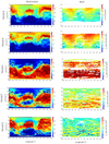 |
Fig. 5 Left: 2D maps of the average illumination of the surface during the periods A, B, E, F, and G described in Table 1, based on the average subsolar latitude and the heliocentric distance. Colors give the normalized intensity, maxima in red and minima in blue. Right: spatial heterogeneities of RTOF H2O number densities (log 10) in cm−3 projected onto the SSC point, and scaled to a distance of 1 km from the center of the nucleus, for the seven periods (see Table 1). |
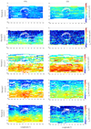 |
Fig. 6 Spatial heterogeneities of RTOF CO2 (left) and CO (right) number densities projected onto the SSC point, and scaled to a distance of 1 km from the center of the nucleus, for the periods A, B, E, F, and G (see Table 1). |
Number densities of the RTOF main volatiles (scaled to a distance of 1 km) for the seven periods for the northern hemisphere (SSC > 15°).
Number densities of the RTOF main volatiles (scaled to a distance of 1 km) for the seven periods for the southern hemisphere (SSC < −15°).
3.2.3 Dichotomy between the two hemispheres
The dichotomy between the two lobes has been investigated by defining two areas of 20° of latitude and 30° of longitude, centered on (0,0) over the small lobe and centered on (145,0) over the large lobe. From the entire dataset, we calculated the following median ratios: CO2/H2O = 0.19; CO/H2O = 0.32 for the small lobe, and CO2/H2O = 0.32; CO/H2O = 0.38 for the large lobe, with standard deviations from 0.6 to 1. This shows that the ratio CO/H2O is practically identical between the two lobes, while there is a difference for the CO2/H2O ratio. However, we can hardly conclude on a differential lobe composition for CO2 because of the large dispersion and also because the hemispherical asymmetries are strong and the dynamics of the coma measurements are complex. Moreover, these ratios do not reflect the relative production over the whole apparition because not all the periods were covered with the exact same measurements conditions.
3.3 Detection of O2
In a typical cleaned RTOF spectra (Fig. 1 of Paper I), numerous peaks can be observed. In addition to the three largest peaks H2O, CO2, and CO, RTOF was able to detect minor species such as the peak at mass/charge 32 u e−1, shown in Fig. 7. Nevertheless, O2 in RTOF spectra needs to be studied with caution. Considering its mass resolution, RTOF is not able to distinguish different species with close m/q ratios. In addition, three of the molecules detected on comet are tentatively detected in the peak at mass 32: molecular oxygen (31.999 amu e−1), sulfur (32.065 amu e−1), and methanol (32.042 amu e−1).
Two methods were used to overcome this problem. The first is the identification of the parent molecules. The high time-resolution of RTOF, with an entire spectrum acquired every 200 s, enables us to simultaneously measure parent and daughter molecules, which is not possible with DFMS. For example, H2 S being the major contributor to sulfur, the analysis of the peak at mass/charge 34 u e−1 can provide us information on the contribution to the atomic sulfuric at mass/charge 32 u e−1. This information, along with DFMS data, enables us to study molecular oxygen as seen by RTOF when the sulfur and methanol compounds are negligible. This constraint does not allow us to provide a temporal and spatial study throughout the full mission, as provided for H2O, CO2, and CO. Here, we present results of the O2 density for period A.
The data analysis is the same as explained in Sect. 2.2, except that the ground calibration of RTOF in order to obtain the O2 sensitivity was not available. Therefore, the sensitivity used to obtain density values was estimated using the correlation between sensitivity and ionization cross sections, as explained in Gasc et al. (2017b). During the period A, we measured a mean value of 8.7% and a median value of 4.9% for O2 relative to H2O. This value is in the range 1–10% measured by ROSINA/DFMS from September 2014 to March 2015, although they obtained a lower mean value of 3.8% (Bieler et al. 2015). We note that ALICE on ROSETTA measured an O2 relative abundance to H2O, derived from an absorption stellar spectrum, ranging from 11 to 68% (Keeney et al. 2017). The difference between the mass spectrometric and the optical measurements has not been completely explained so far and is probably related to the fact that ALICE does not observe O2, but atomic oxygen from dissociation of O2. The production of excited O is difficult to estimate because photons and energetic electrons contribute to it.
The correlation between O2 and H2O is weaker than that from DFMS results (Bieler et al. 2015): we obtain a Pearson correlation coefficient of 0.42. Nonetheless, this could be the effect of neglecting CH3OH and S, which are present in DFMS spectra. Another reason is that the dispersion of the O2 signal seen by RTOF is higher than that detected by DFMS because the time resolution is higher. Moreover, we were able to observe the spatial variations ofO2 during period A, as shown in Fig. 8. The sublimation of molecular oxygen is very well correlated with illumination and water sublimation because the northern hemisphere appears to be more active than the southern hemisphere. The neck region also shows more O2 outgassing than the lobes.
 |
Fig. 7 Typical RTOF spectrum in abundance (ions/sec) zoomed to the mass per charge range [30,34] showing a peak at mass/charge32 u e−1. The gaps represent electronic noise peaks that were removed. |
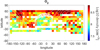 |
Fig. 8 Spatial heterogeneities of O2 density (scaled to a distance of 1 km) in cm−3 km2 during period A. |
4 Discussion
While H2O represents the first contributor to the gas activity during most of the mission, the CO2 and CO outgassing contributions overall increased in the last months, and CO2 became the dominant volatile after the second equinox. When we take the nadir approximation we used here and the delay between illumination and detection of volatiles in the coma into account, the water sublimation is spatially well correlated with the illumination, with a maximum located around the neck of the comet. After perihelion until the end of mission, the total outgassing decreased as the comet moved away from the Sun. The comparison of the situation before the first and after the scond equinox shows a completely different spatial distribution: the southern hemisphere is globally more active at the end of the mission. The illumination conditions and heliocentric distances are comparable, but as the thermal conductivity near the surface is low, the heat remains longer in the interior, and the sublimation of H2O (and other volatiles as well) in the southern hemisphere is prolonged.
The behavior of CO and CO2 is more complex because the sublimation of CO and CO2 does not follow the illumination conditions (correlation factors lower than 0.27). First, an overall dichotomy between thenorthern and southern hemisphere clearly appears in the number density maps. Such a dichotomy could be induced by the insulation of the northern hemisphere by a dust layer transported from the south to the north during the previous perihelion (Keller et al. 2015), thus reducing the sublimation of CO and CO2 in the north. The complex variations in the ratios in Fig. 2 is detailed by splitting the set of data according to the hemisphere. Figure 9 shows CO2/H2O and CO/H2O ratios for the entire mission, for the SSC point latitudes above than 15° (northern hemisphere) and below than −15° (southern hemisphere). The number density ratios for both hemispheres are given in Table 6. In the northern hemisphere, the CO/H2O ratio is equal to or higher than the CO2/H2O ratio for almost the entire mission, while variations in the southern hemisphere ratios are more complex. In the northern hemisphere, we recorded averaged ratios from 0.04 (period D) to 0.22 (period G) for CO2/H2O and from 0.04 (period B) to 0.3 (period A) for CO/H2O. In comparison, we obtain averaged ratio from 0.04 (period C) to 1.34 (period G) for CO2/H2O and from 0.1(period C) to 1.19 (period G) for CO/H2O in the southern hemisphere. We note that CO spatial maps are in general more homogeneous because CO molecules have the lowest sublimation temperature, the first layer containing CO is located deeper, and the detections depend less strongly on the seasonal variations.
Second, in the northern hemisphere, CO and CO2 have a cyclic outgassing behavior: a medium outgassing rate during period A, a very low rate during period B, a highest rate during period E, a medium rate during period F, and a low rate during period G. The highest sublimation appears at the end of summer in the southern hemisphere. Two scenarii are examined to explain this observation:
– We introduce an hypothesis about the near-surface structure of the nucleus. Cometary nuclei are described as icy conglomerates or aggregates of pre-solar grains covered by an ice layer. Insolation mainly drives sublimation of ices, which leads to a layering of the upper layers of the nucleus, and to the appearance of a layer of dust over the ices (Grün et al. 1989; Greenberg 1998; Greenberg & Li 1999). Observations and grain analysis confirmed a nonvolatile layer on the surface of 67P, which locally reduced the activity (Schulz et al. 2015; Gundlach et al. 2015). From these descriptions of a nucleus, we propose a structure of the northern near-surface nucleus: first a dust layer containing water ice, then a layer of pure water ice, and finally CO and CO2 located underneath. Far from the Sun, the temperature at the surface is at first high enough to sublimate CO and CO2 but not H2O. Approaching the Sun, the temperature then rises at the surface, allowing the water ice contained in the dust to sublimete, but because the temperature drops rapidly with depth, the temperature is too low to sublimate the pure water ice layer, allowing the CO and CO2 that is located underneath to be sublimated (period A). At lower heliocentric distances, the temperature in the interior then increases until it is sufficient to induce the sublimation of the pure water-ice layer. This process consumes a large part of the available energy, and the CO and CO2 fluxes drop in the northern hemisphere (pre-equinox one period) until perihelion, where the heat wave again reaches CO and CO2.
– The cyclic outgassing behavior of CO and CO2 in the northern hemisphere could otherwise be explained if CO and CO2 were included in the wet icy dust layer. The dust material is ejected from the southern hemisphere, where CO and CO2 may be close to the surface. The ejected dust containing water could also have carried CO and CO2 if the species were trapped previously. These ice species would thus be sublimated and emptied during periods A and B, leading to the observed CO and CO2 flux decrease until the sublimation of the deeper layers dominates before perihelion. This hypothesis requires the ejection of large dust particles that are capable of retaining CO and CO2 molecules until the redeposition in the northern hemisphere. CO would have to be retained for several hours of flight time during the strong heating, during the transport around perihelion, and until >3 au inbound. Moreover, dust particles arenot expected to be large enough, as estimated in Keller et al. (2017), thus this scenario appears less probable.
In the southern hemisphere, CO2 and CO sublimation is observed without particular correlations with water detections. The active zones sublimating CO seem to overlap the zones sublimating CO2 in the RTOF dataset. The strong heating eroded the southern hemisphere more intensely during the summer. This erosion gave access to deeper layers, containing CO2 and CO, and allows us to detect them more intensely than in the northern hemisphere.
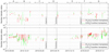 |
Fig. 9 Time evolution of the CO/H2O and CO2/H2O density ratios for the entire mission for the northern (upper panel) and southern (lower panel) hemisphere. |
5 Conclusions
We analyzed the full ROSINA/RTOF dataset during the Rosetta mission, from September 2014 until September 2016, for the three main volatiles H2O, CO2, and CO. The previous analysis of ROSINA data revealed strong periodicities in time and heterogeneities throughout the surface of 67P during the first part of the mission (Hässig et al. 2015; Hoang et al. 2017). We here extended these studies to the entire RTOF dataset and focused in particular on the evolution of the north-south dichotomy through the cometary seasons.
The global outgassing of 67P changed with heliocentric distance, with an asymmetry with respect to perihelion. We observed large changes in relative abundances between the beginning and the end of mission. This revealed a different behavior of the species ratios, with an increasing contributionof CO2 and CO in the total outgassing toward the end of the mission.
This work allowed us to compare the activity of the comet over several periods: during the approach, around the first equinox, around perihelion, and around the second equinox. The spectra recorded throughout the escort phase show an active nucleus for the three volatiles. The H2O outgassing rate essentially follows the illumination conditions, while the CO/H2O and CO2/H2O ratios are maxima already far from the Sun because of the higher volatility of CO and CO2. However, these two volatiles show complex behaviors when the seasonal variability and the spatial heterogeneities are investigated. Their relative abundance (CO/CO2) is also variable, from below 1 (in agreement with CO2 being close to the surface) to above 1 (expected at large distances because the sublimation temperature of CO is lower). Observations of H2O and CO2 made by the VIRTIS instrument agreed with these changes in outgassing composition observed with RTOF, as Bockelée-Morvan et al. (2016) reported an increase of CO2/H2O ratio by a factor of 2 to reach 32% just after perihelion.
Mapping the RTOF detections to the SSC point on the nucleus shows that H2O, CO2, and CO originate from all regions of the comets, regardless of illumination. The data from the extremities of the two lobes at first suggest a possible intrinsic difference in CO2 composition between the upper layers of the two lobes. However, after careful analysis, the origin of the detections mostly depends on the seasons and on the hemisphere that is observed.
During the first two periods, water detections originated from the northern hemisphere, in particular, the neck region. The MIRO instrument also recorded the highest column density in the neck region in September 2014 (Gulkis et al. 2015; Marshall et al. 2017; Biver et al. 2019), such as the ALICE spectrograph in late 2014 (Feldman et al. 2015). Around perihelion, MIRO localized the most active regions in the southern hemisphere, in particular Wosret, Neith, and Bes, which agreed well with the RTOF post-perihelion detections. As for the other Rosetta instruments, we observed that the regions receiving the highest amount of solar illumination globally presented the highest water production rate, and that outgassing was still observed in recently shadowed areas, like during period G. VIRTIS also observed that the water distribution is well described by the illumination condition, while the distribution of CO2 is not only affected by the illumination conditions, but also by the illumination history (Fink et al. 2016). Fink et al. (2016) detected CO2 that essentially originated from the southern hemisphere, which is likely more eroded (and thus pristine) because this hemisphere was strongly illuminated during the previous perihelion. If the water pattern correlates well with the illumination, it is indeed more complex for CO2 and CO.
The southern hemisphere in particular sublimates more CO and CO2 than the northern hemisphere. CO and CO2 ices are probably very close to the surface in the south and easily sublimated when the temperature is high enough, which is in agreement with the observed strong erosion of the southern hemisphere between the equinoxes. The dichotomy can be induced by an insulating layer of dust containing water ice that is transported from the south (at the previous perihelion period) to the north, which would decrease the northern CO and CO2 fluxes after perihelion. A differential composition (CO/H2O and CO2/H2O ratios) between the two hemispheres could also lead to such a dichotomy, but would be more difficult to explain.
Nevertheless, we do observe CO and CO2 molecules originating from the northern hemisphere, whose fluxes strongly decrease during the pre-equinox period, while the H2O fluxes increase. The presence of a wet icy dust layer cannot explain this behavior. One interpretation could be based on the stratigraphy of the near-surface part of the nucleus, which might be composed of a dust layer containing water ice, then a layer of pure water ice, and finally CO and CO2 located deeper. When the comet is far from the Sun, the temperature increase is not sufficient to sublimate water, but the heat wave propagates inside the nucleus and sublimates CO and CO2. During period A, the increase in temperature leads to the sublimation of water contained in the insulating dust layer. As the temperaturedrops with depth, the heat wave cannot sublimate the pure water-ice layer, but is able to sublimate the CO2 and CO located underneath. Closer to the Sun, in the pre-equinox one period, the temperature is sufficient to sublimate the pure water-ice layer. The available energy is almost consumed by this process, and the fluxes of CO and CO2 drop until perihelion, where the temperature strongly increases and the heat wave can propagate to the deeper layers, where it again induces the sublimation of CO2 and CO.
The preliminary study of minor species with RTOF brought results for O2, confirming the independent detection from ALICE (Feldman et al. 2015) and ROSINA/DFMS (Bieler et al. 2015), with a mean value relative to water within the range measured by DFMS. However, this study requires further investigations and has to be made with caution because of the mass resolution of RTOF and the uncertainty on the sensitivity values of the minor species.
In the near future, our aim is to compare the ROSINA coma detections during the mission with the outgassing rate derived from a nucleus model. Cross comparisons, assuming several scenarii as discussed above, will help to constrain the internal structure of the comet, such as its stratigraphy, or to find answers to the unknown nature of the gas trapping. They might also indicate whether significant amounts of amorphous ice are present.
Acknowledgements
The authors thank the following institutions and agencies that supported this work. Work at IRAP was supported by the French space agency CNES. Work at the University of Bern was funded by the State of Bern, the Swiss National Science Foundation, and the European Space Agency PRODEX Programme. Work at the Max Planck Institute for Solar System Research was funded by the Max-Planck Society and Bundesministerium für Wirtschaft und Energie under contract 50QP1302. The results from ROSINA would not be possible without the work of the many engineers, technicians, and scientists involved in the mission, the Rosetta spacecraft, and the ROSINA instrument team over the past 20 yr, whose contributions are gratefully acknowledged. Rosetta is an European Space Agency (ESA) mission with contributions from its member states and NASA. We thank herewith the work of the whole ESA Rosetta team. All ROSINA flight data have been or will be released to the PSA archive of ESA and to the PDS archive of NASA. The authors thank D. Toublanc for developing the illumination code that was applied on the cometary nucleus.
References
- Accomazzo, A., Ferri, P., Lodiot, S., et al. 2017, Acta Astronaut., 136, 354 [NASA ADS] [CrossRef] [Google Scholar]
- Balsiger, H., Altwegg, K., Bochsler, P., et al. 2007, Space Sci. Rev., 128, 745 [NASA ADS] [CrossRef] [Google Scholar]
- Barucci, M. A., Filacchione, G., Fornasier, S., et al. 2016, A&A, 595, A102 [NASA ADS] [CrossRef] [EDP Sciences] [Google Scholar]
- Bieler, A., Altwegg, K., Balsiger, H., et al. 2015, Nature, 526, 678 [Google Scholar]
- Biver, N., Bockelée-Morvan, D., Hofstadter, M., et al. 2019, A&A, 630, A19 (Rosetta 2 SI) [NASA ADS] [CrossRef] [EDP Sciences] [Google Scholar]
- Bockelée-Morvan, D., Debout, V., Erard, S., et al. 2015, A&A, 583, A6 [NASA ADS] [CrossRef] [EDP Sciences] [Google Scholar]
- Bockelée-Morvan, D., Crovisier, J., Erard, S., et al. 2016, MNRAS, 462, S170 [Google Scholar]
- Capaccioni, F., Coradini, A., Filacchione, G., et al. 2015, Science, 347, aaa0628 [Google Scholar]
- De Sanctis, M., Capaccioni, F., Ciarniello, M., et al. 2015, Nature, 525, 500 [NASA ADS] [CrossRef] [Google Scholar]
- El-Maarry, M., Thomas, N., Giacomini, L., et al. 2015, A&A, 583, A26 [NASA ADS] [CrossRef] [EDP Sciences] [Google Scholar]
- El-Maarry, M. R., Thomas, N., Gracia-Berná, A., et al. 2016, A&A, 593, A110 [NASA ADS] [CrossRef] [EDP Sciences] [Google Scholar]
- Feldman, P. D., A’Hearn, M. F., Bertaux, J.-L., et al. 2015, A&A, 583, A8 [NASA ADS] [CrossRef] [EDP Sciences] [Google Scholar]
- Filacchione, G., Capaccioni, F., Ciarniello, M., et al. 2016, Icarus, 274, 334 [NASA ADS] [CrossRef] [Google Scholar]
- Fink, U., Doose, L., Rinaldi, G., et al. 2016, Icarus, 277, 78 [NASA ADS] [CrossRef] [Google Scholar]
- Gasc, S., Altwegg, K., Balsiger, H., et al. 2017a, MNRAS, 469, S108 [Google Scholar]
- Gasc, S., Altwegg, K., Fiethe, B., et al. 2017b, Planet. Space Sci., 135, 64 [NASA ADS] [CrossRef] [Google Scholar]
- Greenberg, J. M. 1998, A&A, 330, 375 [NASA ADS] [Google Scholar]
- Greenberg, J. M., & Li, A. 1999, Space Sci. Rev., 90, 149 [NASA ADS] [CrossRef] [Google Scholar]
- Grün, E., Bar-Nun, A., Benkhoff, J., et al. 1989, IAU Colloq. 116, 277 [NASA ADS] [Google Scholar]
- Gulkis, S., Allen, M., von Allmen, P., et al. 2015, Science, 347, aaa0709 [Google Scholar]
- Gundlach, B., Blum, J., Keller, H., & Skorov, Y. 2015, A&A, 583, A12 [NASA ADS] [CrossRef] [EDP Sciences] [Google Scholar]
- Hansen, K. C., Altwegg, K., Berthelier, J.-J., et al. 2016, MNRAS, 462, S491 [Google Scholar]
- Hässig, M., Altwegg, K., Balsiger, H., et al. 2015, Science, 347, aaa0276 [Google Scholar]
- Hoang, M., Altwegg, K., Balsiger, H., et al. 2017, A&A, 600, A77 [NASA ADS] [CrossRef] [EDP Sciences] [Google Scholar]
- Jorda, L., Gaskell, R., Capanna, C., et al. 2016, Icarus, 277, 257 [NASA ADS] [CrossRef] [Google Scholar]
- Keeney, B. A., Stern, S. A., A’hearn, M. F., et al. 2017, MNRAS, 469, S158 [CrossRef] [Google Scholar]
- Keller, H. U., Mottola, S., Davidsson, B., et al. 2015, A&A, 583, A34 [NASA ADS] [CrossRef] [EDP Sciences] [Google Scholar]
- Keller, H. U., Mottola, S., Hviid, S. F., et al. 2017, MNRAS, 469, S357 [CrossRef] [Google Scholar]
- Le Roy, L., Altwegg, K., Balsiger, H., et al. 2015, A&A, 583, A1 [NASA ADS] [CrossRef] [EDP Sciences] [Google Scholar]
- Marshall, D., Hartogh, P., Rezac, L., et al. 2017, A&A, 603, A87 [NASA ADS] [CrossRef] [EDP Sciences] [Google Scholar]
- Massironi, M., Simioni, E., Marzari, F., et al. 2015, Nature, 526, 402 [NASA ADS] [CrossRef] [Google Scholar]
- Migliorini, A., Piccioni, G., Capaccioni, F., et al. 2016, A&A, 589, A45 [NASA ADS] [CrossRef] [EDP Sciences] [Google Scholar]
- Pommerol, A., Thomas, N., El-Maarry, M. R., et al. 2015, A&A, 583, A25 [NASA ADS] [CrossRef] [EDP Sciences] [Google Scholar]
- Scherer, S., Altwegg, K., Balsiger, H., et al. 2006, Int. J. Mass Spectrom., 251, 73 [NASA ADS] [CrossRef] [Google Scholar]
- Schulz, R., Hilchenbach, M., Langevin, Y., et al. 2015, Nature, 518, 216 [NASA ADS] [CrossRef] [Google Scholar]
- Sierks, H., Barbieri, C., Lamy, P. L., et al. 2015, Science, 347, aaa1044 [Google Scholar]
- Taylor, M., Altobelli, N., Buratti, B., & Choukroun, M. 2017, Phil. Trans. R. Soc. A, 375, 20160262 [CrossRef] [Google Scholar]
All Tables
Description of the seven periods covering the RTOF dataset, with the corresponding heliocentric distances and the average subsolar latitudes.
Number densities of the RTOF main volatiles (scaled to a distance of 1 km) for the seven periods for the northern hemisphere (SSC > 15°).
Number densities of the RTOF main volatiles (scaled to a distance of 1 km) for the seven periods for the southern hemisphere (SSC < −15°).
All Figures
|
Fig. 1 Upper panel: temporal evolution of H2O, CO2, and CO densities multiplied by the cometocentric distance squared, derived from RTOF relative abundances scaled to COPS over the Rosetta mission. Colored lines are averaged over two comet rotations. Middle panel: latitude of the sub-spacecraft point in the 67P fixed frame. Lower panel: variation in distance between Rosetta and 67P (black) and the heliocentric distance (yellow). First equinox occurred on 2015 May 10 at 1.67 au, perihelion on 2015 August 13 at 1.24 au, andsecond equinox on 2016 March 21 at 2.63 au. RTOF data are missing during excursions of the spacecraft. Periods A to G are indicated above the first panel. They are described in Table 1. |
| In the text | |
|
Fig. 2 Upper panel: time evolution of CO/H2O and CO2 /H2O density ratios for the entire mission, starting in September 2014 and ending in September 2016. Lower panel: variation in SSC point latitude in degrees. Periods A to G are indicated above the first panel, and they are described in Table 1. |
| In the text | |
|
Fig. 3 Left: temporal evolution after equinox of the densities of the RTOF (first panel) and DFMS main volatiles (second panel) with the average over two comet rotations (colored lines), the COPS nude gauge total densities (third panel), and the SSC point latitude and longitude (fourth panel). Right: zoom-in on one rotation (~12 h). |
| In the text | |
|
Fig. 4 Number densities of the main volatiles for the five last days of RTOF measurements (upper panels) and corresponding SSC latitude and longitude (lower panels). |
| In the text | |
|
Fig. 5 Left: 2D maps of the average illumination of the surface during the periods A, B, E, F, and G described in Table 1, based on the average subsolar latitude and the heliocentric distance. Colors give the normalized intensity, maxima in red and minima in blue. Right: spatial heterogeneities of RTOF H2O number densities (log 10) in cm−3 projected onto the SSC point, and scaled to a distance of 1 km from the center of the nucleus, for the seven periods (see Table 1). |
| In the text | |
|
Fig. 6 Spatial heterogeneities of RTOF CO2 (left) and CO (right) number densities projected onto the SSC point, and scaled to a distance of 1 km from the center of the nucleus, for the periods A, B, E, F, and G (see Table 1). |
| In the text | |
|
Fig. 7 Typical RTOF spectrum in abundance (ions/sec) zoomed to the mass per charge range [30,34] showing a peak at mass/charge32 u e−1. The gaps represent electronic noise peaks that were removed. |
| In the text | |
|
Fig. 8 Spatial heterogeneities of O2 density (scaled to a distance of 1 km) in cm−3 km2 during period A. |
| In the text | |
|
Fig. 9 Time evolution of the CO/H2O and CO2/H2O density ratios for the entire mission for the northern (upper panel) and southern (lower panel) hemisphere. |
| In the text | |
Current usage metrics show cumulative count of Article Views (full-text article views including HTML views, PDF and ePub downloads, according to the available data) and Abstracts Views on Vision4Press platform.
Data correspond to usage on the plateform after 2015. The current usage metrics is available 48-96 hours after online publication and is updated daily on week days.
Initial download of the metrics may take a while.