| Issue |
A&A
Volume 630, October 2019
|
|
|---|---|---|
| Article Number | A129 | |
| Number of page(s) | 12 | |
| Section | Numerical methods and codes | |
| DOI | https://doi.org/10.1051/0004-6361/201834180 | |
| Published online | 04 October 2019 | |
A well-balanced scheme for the simulation tool-kit A-MaZe: implementation, tests, and first applications to stellar structure
1
Centre de Recherche Astrophysique de Lyon UMR5574, Univ. Lyon, Ens de Lyon, Univ. Lyon1, CNRS, 69364 Lyon Cedex 07, France
e-mail: This email address is being protected from spambots. You need JavaScript enabled to view it.
2
College of Engineering, Mathematics and Physical Sciences, University of Exeter, Exeter EX4 4QL, UK
3
Department of Physics and Astronomy, Georgia State University, Atlanta, GA 30303, USA
4
Seminar of Applied Mathematics, ETH-Zürich, Switzerland
Received:
3
September
2018
Accepted:
30
August
2019
Abstract
Characterizing stellar convection in multiple dimensions is a topic at the forefront of stellar astrophysics. Numerical simulations are an essential tool for this task. We present an extension of the existing numerical tool-kit A-MaZe that enables such simulations of stratified flows in a gravitational field. The finite-volume based, cell-centered, and time-explicit hydrodynamics solver of A-MaZe was extended such that the scheme is now well-balanced in both momentum and energy. The algorithm maintains an initially static balance between gravity and pressure to machine precision. Quasi-stationary convection in slab-geometry preserves gas energy (internal plus kinetic) on average, despite strong local up- and down-drafts. By contrast, a more standard numerical scheme is demonstrated to result in substantial gains of energy within a short time on purely numerical grounds. The test is further used to point out the role of dimensionality, viscosity, and Rayleigh number for compressible convection. Applications to a young sun in 2D and 3D, covering a part of the inner radiative zone, as well as the outer convective zone, demonstrate that the scheme meets its initial design goal. Comparison with results obtained for a physically identical setup with a time-implicit code show qualitative agreement.
Key words: methods: numerical / stars: interiors / hydrodynamics / convection
© M. V. Popov et al. 2019
 Open Access article, published by EDP Sciences, under the terms of the Creative Commons Attribution License (http://creativecommons.org/licenses/by/4.0), which permits unrestricted use, distribution, and reproduction in any medium, provided the original work is properly cited.
1. Introduction
In a wide range of astrophysical objects, the balance between gravitation and gas pressure is a key element, on top of which additional physics may take place. Ascertaining the robustness of corresponding numerical results, by applying different codes to the same physical problem, is a motivation behind this paper on the adaptation of the A-MaZe tool-kit (Walder & Folini 2000; Folini et al. 2003; Melzani et al. 2013) so that it can tackle gravitationally stratified flows.
Stars and planets are prominent astrophysical examples harboring such flows. Although quasi-static in a global sense, a wealth of dynamics takes place. Energy transport via convection is often essential in maintaining a globally quasi-static state. This is notably the case for the outer parts of low mass stars and the inner regions of high mass stars, where energy transport via radiation is not efficient enough. Multidimensional simulations of such transport processes contribute to the 321D link for stellar modeling (e.g., Arnett et al. 2015), that is, the effort to improve one-dimensional stellar evolution models via simulating short episodes in 2D and 3D. These studies motivate the overall project into which this study is embedded (see e.g., Geroux et al. 2016; Pratt et al. 2017; Baraffe et al. 2017). Other examples exist where the pressure-gravity balance plays a crucial role and associated numerical challenges resemble the ones we are interested in here. We mention the vertical structure of accretion disks and supernova explosions, notably the moment just before the onset of the collapse and then again when the prompt shock stalls (Couch & Ott 2013; Müller et al. 2016, 2017).
From a numerical point of view, the above astrophysical problems are challenging because the gravity and pressure forces, which are both typically large but of opposite sign, may not cancel out in their discretized form. This non-cancellation may severely impact the solution. A number of remedies have been suggested (for a short overview, see e.g., Käppeli & Mishra 2016). Here we focus on so called well-balanced schemes, that is, schemes which are designed to exactly maintain a discrete equivalent of the underlying stationary state. Initially put forward by Cargo & LeRoux (1994) and Greenberg & Leroux (1996), numerous concrete forms of well-balanced schemes meanwhile exist (LeVeque 1998; Noelle et al. 2009; Wang et al. 2009; Xing & Shu 2013; Käppeli & Mishra 2014, 2016; Chandrashekar & Klingenberg 2015; Berberich et al. 2017; Desveaux et al. 2016; Touma et al. 2016). Major differences among them include the allowed equation of state (EoS), roughly speaking “simple” or “complicated,” whether the EoS explicitly enters the well-balanced reconstruction or not, the required knowledge about the stationary state (from “analytical form” to “none at all”), whether the method is designed for shallow water problems or the full Euler or Navier–Stokes equations, and whether the scheme relies on velocities being (and remaining) zero or not.
The goal of this paper is to document the implementation of a well-balanced scheme into the A-MaZe simulation tool-kit, to demonstrate its performance with a series of tests, to illustrate the behavior of a not well-balanced scheme for the same tests, and to draw attention to selected physical aspects of the tests.
As our primary interest is with stellar convection, we want a well-balanced scheme that is applicable to the full Euler or Navier–Stokes equations, works for flows in external gravitational fields and for self-gravitating flows, can cope with an arbitrary EoS, does not rely on prior knowledge of the stationary state, and can accommodate non-zero velocities. The scheme should be simple enough so that it can be easily accommodated in an existing code and, in the future, can be combined with adaptive meshes and general curvilinear grids. With these considerations in mind, we decided for the approach by Käppeli & Mishra (2016; KM16 in the following) as a starting point for our own work; however, we did adapt the treatment of the energy source term.
The paper is structured as follows. In Sect. 2, we present the overall problem along with our algorithm as part of the simulation tool-kit A-MaZe and with particular focus on the well-balanced scheme. A first set of test cases, static configurations, and convective slabs, are examined in Sect. 3. The performance of the algorithm for a test case closer to our finally envisaged applications, featuring in particular a general EoS that is in the form of a look-up table, is demonstrated in Sect. 4. A discussion follows in Sect. 5, and a summary and conclusions are in Sect. 6.
2. Equations and methods
We look for numerical solutions of the compressible Navier–Stokes equations in the presence of a gravitational field, as detailed in Sect. 2.1. Essential aspects of A-MaZe, our hosting numerical tool-kit, are summarized in Sect. 2.2. The well-balanced extension of A-MaZe is detailed in Sect. 2.3.
2.1. Navier–Stokes equations with gravity
The Navier–Stokes equations for a thermally conductive and compressible medium in the presence of a gravitational potential ϕ can be written as a system of balance laws in the form
 (1)
(1)
 (2)
(2)
 (3)
(3)
with
 (4)
(4)
the gas energy density, ρ the density, u the velocity vector, p the gas pressure, e the specific internal energy, K the (potentially nonlinear) heat-transfer coefficient, and T the temperature. The components of the dynamic viscous stress tensor, denoted τ, are defined as
 (5)
(5)
where μ is the dynamic viscosity (volume or bulk viscosity is neglected). The EoS as well as μ and K, are problem specific and, consequently, are further specified along with the test cases in Sects. 3 and 4.
Throughout the paper we neglect changes of gravity due to matter re-distribution. We assume a problem specific but time-constant gravitational potential ϕ with associated free-fall acceleration vector g
 (6)
(6)
Hydrostatic equilibrium is therefore defined by
 (7)
(7)
The gravitational energy density Eg of the gas is given by
 (8)
(8)
Two characteristic time scales are the sound crossing time
 (9)
(9)
and the convective turnover time τc
 (10)
(10)
The integral extends over a characteristic length scale, e.g a scale height or the depth of convection zone (here in x-direction). The local (at distance x) sound speed, Mach number, and flow velocity in direction of g are denoted by cs(x), M(x), and ux(x), respectively, and  is the depth-averaged Mach number. In many astrophysically relevant cases, the convective motion is very subsonic and thus τc > > τs. For instance, in their study of a young sun in 2D with M ≤ 0.05, Pratt et al. (2016) needed an integration time of several hundred τc, translating into several thousand τs, for robust statistics. This sets the time scale of interest, over which Eqs. (1)–(3) have to be integrated numerically.
2.2. Numerical tool-kit A-MaZe
We build on the numerical tool-kit A-MaZe (Walder & Folini 2000; Folini et al. 2003; Melzani et al. 2013), a collection of adaptive mesh (Berger & Oliger 1984; Berger & Colella 1989; Folini et al. 2003) multi-scale, multi-physics codes and analysis tools to support simulations of astrophysical objects. A-MaZe has been applied to a range of problems, including accretion and blasts in novas (Walder et al. 2008), full scale simulations of X-ray binaries (Walder et al. 2014), colliding winds and emitted spectra (Nussbaumer & Walder 1993; Folini & Walder 1999, 2000), particle acceleration in relativistic magnetic reconnection (Melzani et al. 2014a,b), investigation of supersonic turbulence (Folini & Walder 2006; Folini et al. 2014), and the dynamics of circum-stellar material (Folini et al. 2004; Georgy et al. 2013).
Until now, A-MaZe lacked a proper treatment of a static balance between gravitational and pressure forces. The present paper remedies this shortcoming by appropriately augmenting (see Sect. 2.3) the hydrodynamic solver. Key characteristics of the latter, as far as relevant for and used in this paper, are summarized in the following.
Equations (1)–(3) are solved using a finite volume discretization on the basis of mapped grids (Calhoun et al. 2008) for general curvi-linear coordinates. A regular Cartesian mesh (the computational mesh) is mapped to the desired mesh in physical space (the physical mesh). Within this paper, physical meshes are truly Cartesian (in 1D, 2D, and 3D), 2D axi-symmetric, or 3D spherical shell wedges. Other mappings have not yet been implemented, although the code infrastructure to hold them is in place. As the concrete mapping functions depend on the specific application, they are formulated in the context of the latter in Sect. 3. Advective fluxes through the cell faces are computed with the help of a Riemann-solver, which feeds on data at cell interfaces (left and right state, at the geometrical center of the interface) obtained by standard (limited) reconstruction techniques. Within the context of mapped grids, advective as well as diffusive fluxes can be computed on the computational mesh, with the physical mesh entering only via cell surface areas and cell volumes. This procedure avoids geometrical source terms (see e.g., Kifonidis & Müller 2012, for a more detailed discussion).
The semi-discretized three-dimensional version of Eqs.(1)–(3) is
 (11)
(11)
Here, 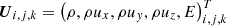 is the vector of conserved quantities at cell centers (i, j, k)∈(1, …, Nx, 1, …, Ny, 1, …, Nz), with Nx, Ny, and Nz the number of cells in x-, y-, and z-direction of computational space. Half indices denote cell faces. Fi ± 1/2, j, k, Gi, j ± 1/2, k, and Hi, j, k ± 1/2 denote the fluxes through the cell faces. We note that they contain advective and diffusive terms. Physical space enters only via the cell surfaces (terms Si ± 1/2, j, k) and cell volumes (terms Vi, j, k), both evaluated in physical space, as well as via the source term Ψi, j, k, also evaluated in physical space.
Time integration of Eq. (11) in this paper is done with a first order Runge–Kutta method (a forward Euler method), although A-MaZe also offers strong stability preserving (SSP) higher order integration schemes (Shu & Osher 1988; Gottlieb et al. 2001). We used different Riemann solvers, notably the approximate HLLC (Toro et al. 1994), as well as the exact solver by Colella & Glaz (1985). Likewise, we used both minmod and van Leer limiters together with second order reconstruction. Results seem overall robust to the particular choice of integrator and limiter, but no detailed analysis in this respect was done. Diffusive fluxes are approximated by a dimensionally split second order central finite difference discretization in space, that is, each spatial direction is treated independently of the others. In the following, we refer to the above approach as the standard scheme.
A variant better suited for situations with a gravitational field, in the following referred to as well-balanced scheme, is described in Sect. 2.3. The difference between the two schemes is small in terms of code: it concerns only the reconstruction of pressure at cell interfaces and the discretization of the source term on the right hand side of Eq. (3).
2.3. The well-balanced algorithm
Related to the gravitational potential, source terms for momentum and energy, SM and SE, exist on the right hand side of Eqs. (2) and (3), respectively. Thus care must be taken to avoid associated numerical sources or sinks of momentum and energy.
2.3.1. Momentum balance
The momentum equation, Eq. (2), includes the hydrostatic balance equation, Eq. (7), to which it reduces in the case of zero velocities. Unless the numerical scheme respects this balance to machine precision, the momentum equation will suffer from spurious gains or losses of momentum associated with SM.
We adopt the scheme of KM16, the key aspects of which we summarize here. The overarching idea is to arrive at a reconstructed pressure at cell interfaces that is (a) identical on the left and right side of the interface and (b) respects a discrete version of the hydrostatic equilibrium equation, Eq. (7). Condition (a) ascertains that the Riemann solver is not fed any spurious pressure jumps that would be translated into waves. Condition (b) ascertains that the pressure gradient across a cell, that is, the pressure contribution to the flux differencing term, matches the source term of the discrete hydrostatic equilibrium. As is stressed in KM16, the equilibrium is a mechanical one, no assumption is made on a thermal equilibrium, that is, no explicit temperature or entropy profile has to be assumed and the hydrostatic equilibrium may be physically unstable to convection. Perturbations on top of the hydrostatic equilibrium pressure are addressed by decomposing the total pressure for the reconstruction as p = p0 + p1, with the hydrostatic part p0 and the perturbation part p1. The well-balanced reconstruction of p0 is second order. For p1 and all other variables, any higher order reconstruction may be used. We use second order in this paper with a minmod limiter.
In 1D (arbitrarily in x-direction) the relevant formulas read as follows. The gravitational source term −ρ ∇ϕ on the right hand side of Eq. (2) is discretized as a centered difference,
 (12)
(12)
The well-balanced reconstruction of the equilibrium part p0 of the pressure of cell i is given by
 (13)
(13)
With  (see condition (a) above), Eq. (13) leads to the discrete, spatially second-order accurate form of the hydrostatic equilibrium equation, Eq. (7),
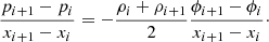 (14)
(14)
The reconstruction of the perturbation part p1 of the pressure (which can be of any order, see KM16) takes as input cell centered values
 (15)
(15)
with
 (16)
(16)
2.3.2. Energy balance
The source term SE in the energy equation, Eq. (3), mediates between the gravitational potential energy Eg of the gas and its internal plus kinetic energy E: as mass is advected along the gravitational field, energy is transferred from Eg to E and vice versa. A numerical pitfall then opens: with ϕ constant in time there is an unlimited reservoir of gravitational energy, thus arbitrary amounts of gas energy may be gained or lost on numerical grounds if SE is not accurately computed. The issue is particularly relevant for quasi-stationary convection, where Eg and E are constant when integrated over the domain of interest, although there is a steady exchange between the two on local scales: in down-flows energy is transferred from Eg to E whereas the opposite is true in regions of up-flow. The numerical scheme must respect the global balance despite the steady local exchange.
In KM16, centered differences are used for the source term in Eq. (3). As we illustrate in Sect. 3, this choice leads to a systematic increase of E with time when simulating quasi-stationary convection. This although there is no net motion of mass in the direction parallel to the gravitational force.
We use an alternative formulation, expressing SE in terms of discrete mass fluxes FM, GM, and KM as
 (17)
(17)
Here, gi + 1/2, j, k = (ϕi + 1, j, k − ϕi, j, k)/(xi + 1, j, k − xi, j, k) etc. The expression for SE can be motivated in two ways. From a physical point of view, one may argue with the connection between the mass flux, projected onto ∇ϕ, and the local exchange between Eg and E. The above equation ascertains that the domain average of  is zero – there is no domain averaged net exchange between E and Eg – unless there is some domain averaged net mass flux parallel to ∇ϕ. Another way to obtain Eq. (17) is to start from a conservative discretization for the total energy Etot = E + Eg, instead of using a source term in the energy equation. This is done, for example, in Jiang et al. (2013). Starting from their equations for the total energy (Eq. (9)), for the energy flux Fg due to gravity (Eq. (14)), and for the update of the energy (Eq. (16)), noting in addition that in our case the gravitational potential ϕ is time constant and the gravitational potential energy is given by Eq. (8), and using for the components of Fg the discrete expressions
  etc. one obtains Eq. (17).
For an individual time step, we expect the difference between our formulation and a centered difference formulation for SE to be small. This is because the mass fluxes at cell interfaces must closely resemble the mass fluxes evaluated at cell centers, the difference arising in essence from the reconstruction (from cell center to cell interface). An analytical error estimate is, however, not trivial as we use the fluxes from the (approximate) Riemann solver. The difference between the two approaches is, however, systematic and thus cumulative over many time steps, at least for a stratified medium in the presence of a fixed gravitational field. The numerical results in Sect. 3 will further underpin this point.
3. Simulating convection: basic tests
Our goal here is twofold: we want to demonstrate that the well-balanced scheme lives up to expectations and we want to illustrate the consequences of using a standard scheme. Section 3.1 focuses on static (zero velocity), marginally stably stratified situations with polytropic EoS in different geometries. Section 3.2 addresses quasi-stationary convection, from 1D to 3D, for an ideal gas EoS. The description of each test follows the same basic scheme: sketch of the physical problem (equations, boundary conditions, analytical solution where possible), information on the numerical domain and its discretization, details on problem initialization and numerical boundary conditions, and, finally, the results of the test.
3.1. Static stratified layers
Tests in this section consist of a stratified medium at rest. Integration in time of such a configuration may or may not preserve its initial, static state, depending on whether the integration scheme is well-balanced or not.
3.1.1. Plane-parallel 1D slab
We repeat one of the tests from KM16, their Sect. 3.1: a hydrostatic 1D plane-parallel atmosphere with gravitational potential ϕ(x) = g x and the EoS of a mono-atomic ideal, isentropic gas, p (ρ, s) = es/cvργ with  . We use g = 1, γ = 5/3, and Rgas = 1. The analytical solution of Eq. (7) under these conditions is given by
 (18)
(18)
For our numerical domain x ∈ [0, 2] pressure scale heights hp(x) = − p/(dp/dx) range from hp(0) = 1 to hp(2) ∼ 0.578. Meshes range from 64 cells to 1024 cells. Thermal and viscous diffusion terms are set to zero in the numerical solution.
As our goal is to test whether our well-balanced scheme can maintain to machine precision a configuration that is initially stratified and at rest, we must ascertain that the initialization satisfies Eq. (14), the discrete counterpart of Eq. (7). To this end, we anchor our discrete solution at the lower domain boundary, where we set ρ0 = 1 and p0 = 1 (implying s0 = 0). We then use a Newton–Raphson method to integrate Eq. (14) together with the above EoS toward the upper domain boundary. The velocity is set to zero everywhere.
Two sets of numerical boundary conditions are used, employing again the Newton–Raphson method to integrate the analytical solution (given here by Eqs. (14) and (18)) from the last within domain cell to fill the ghost cells before each time step. The bottom boundary is reflecting in both cases. The top boundary is set to one or the other of two possible choices. The first possible choice we denote by “free-float”: the current density and pressure profile is extrapolated, velocities are copied from within the domain. The second possible choice we denote by “historical”: the initial density and pressure profile is extrapolated, velocities are set to zero. The free-float boundary conditions correspond to boundary conditions as used in KM16. The historical boundary conditions are a variant thereof, designed to draw the boundaries in each time step to the initial state.
Using the standard scheme, average velocities are around 10−6–10−4 after only 2 τs. The sound speed, for comparison, is around one. In KM16 a more detailed error analysis of these non-zero velocities is given. Here we want to draw attention to a follow up effect: a net transfer of mass toward the upper boundary and a decrease of the mass M(t) of the slab with time, as illustrated in Fig. 1. As can be seen, the mass loss depends on the discretization (more severe for coarser grids) and on the boundary conditions (more severe for free-flow). The well-balanced scheme maintains zero velocities and M(t)/M(0) = 1 to machine precision for both boundary conditions, even for the most coarse discretization of 64 cells.
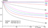 |
Fig. 1. Total mass in 1D hydrostatic slab, normalized by the initial mass (M(t)/M(t = 0), y-axis), as function of time (x-axis, in τs), integrated with the standard scheme, using either historical (dashed lines) or free-float (solid lines) boundary conditions and different meshes (colors; number of grid cells). The well-balanced scheme maintains M(t)/M(t = 0) = 1 to machine precision in all cases. |
The test demonstrates not only that the well-balanced scheme works as expected, but also that it is necessary: the solution suffers from severe numerical artifacts if the standard scheme is used.
3.1.2. Lane–Emden polytrope in 2D and 3D
Lane–Emden polytropes are a good first approximation for the structure of a star. They are solutions to the Lane–Emden equation (see e.g., Kippenhahn & Weigert 1990),
 (19)
(19)
which follows from the equation of hydrostatic equilibrium in 3D spherical symmetry, dp/dr = −ρ(r)GM(r)/r2, for a polytropic EoS p = ξργ, with γ = 1 + 1/n and n = 1, 2, … the polytrope index. A few analytical solutions are known, for instance for γ = 2 (n = 1), our test case:
 (20)
(20)
Here, r is the radius,  , and f(αr) = ρc sin(αr)/(αr). We use ξ = 1, G = 1, and ρc = 1. The situation is marginally stably stratified.
Our goal is again to test whether the well-balanced scheme can maintain the initial, static situation and how, for comparison, the standard scheme behaves. We consider two geometries: a 2D axi-symmetric mesh as well as a 3D Cartesian mesh. The discretized analytical solution, Eq. (20), exactly satisfies the discrete hydrostatic equilibrium, Eq. (14), for both meshes, thus can be used as numerical initial condition.
In the 2D axi-symmetric case, we map the computational to the physical mesh via the mapping function [x, y, z]→[r, θ, φ], with [0…1, 0…1, Δz]↦[0.19…0.95, 0.25π…0.75π, Δφ]. This produces a spherical wedge with a width of one cell in z-direction. We tested that the result does not depend on the choice of the size of Δφ. The domain is discretized by a regular 2562 mesh. In radial direction, historical and reflecting boundary conditions are used at the top and bottom boundary, respectively (see Sect. 3.1.1). Periodic boundary conditions are used in angular direction.
With the well-balanced scheme, velocities remain zero up to machine precision over several hundred sound crossing times (not shown). With the standard scheme velocities start developing early on. After a few hundred sound crossing times a flow field featuring roll-ups, updrafts, and downdrafts has formed, as illustrated in Fig. 2, top panel. The apparent symmetry of the flow structure merely mirrors the symmetry of the code and the initial conditions. Mach numbers are around 0.0005 on average but exceed 0.001 in substantial portions of the flow (green, yellow, and red arrows). This may not seem dramatic. We recall, however, that sound speeds typically exceed convective velocities by one or two orders of magnitude for the stellar situations of interest here (see Sect. 2). This translates the velocities in Fig. 2, which are of purely numerical origin, into a range between 1% to 10% of typical convective velocities. A serious numerical contamination of the physics to be studied thus seems possible if the standard scheme is used.
 |
Fig. 2. Lane–Emden test case, preservation of initially static configuration. Top panel: using the standard scheme, a convection like velocity field develops. Shown is absolute velocity (from purple to white; sound speed ranging from 0.76 to 1.39) with velocity arrows (rainbow colored according to magnitude) for the axi-symmetric 2562 mesh after 300 τs. Bottom panel: using the well-balanced scheme, an initially static polytrope on a 3D Cartesian mesh (1283, star in a box) is preserved to machine precision. Shown are iso-surfaces in density after 300 τs. They remain perfectly spherical despite the Cartesian grid, because velocities remain zero to machine precision, thanks to the well-balanced scheme. |
Using a uniform 1283 3D Cartesian mesh as physical mesh on a [0, 1]3 domain with historical boundary conditions, we repeated the above exercise. The approach is of interest for simulating entire stars, where spherical coordinates struggle with (coordinate-) singularities in the center and along the z-axis. Our approach, often termed “star in a box”, also suffers from a non-optimal mesh: it is a spherical problem on a physically Cartesian mesh. Nevertheless, an initially static configuration is maintained to machine precision by the well-balanced scheme. Figure 2, bottom panel, shows density after 300 τs. Spherical density contours are perfectly preserved, despite the Cartesian mesh. The standard scheme (not shown) develops jittery density contours, the spherical symmetry is broken, and large scale, convection like velocities develop that reach Mach numbers of about 0.1.
3.2. Convective layers
So far we have looked at stationary situations with zero-velocities (up to machine-precision), implying that the energy source term ρu∇ϕ vanishes as well. In this section, we look at convectively unstable situations that are, nevertheless, in a globally stable equilibrium. The test case, to be detailed below, follows Hurlburt et al. (1984; H84 in the following). It consists of a gravitationally stratified slab in planar geometry with parameters and boundary conditions such that compressible convection develops. In H84, a large test-suite of different 2D cases is presented. We repeat two tests for comparison. We then go beyond H84 by briefly addressing the formation of zonal flows in 2D as well as convection in 3D. These additional tests shall demonstrate that our implementation is fit for 3D and draw attention to a specific 2D flow regime. They are not meant to be a parameter study.
3.2.1. Description of test case
We summarize only some key aspects. A comprehensive description of the test can be found in H84. The test has two free parameters: the assumed stratification of the slab, χ, and the Rayleigh number, R. Quantities are in dimensionless form. Gravity points along the negative y-axis. A perfect mono-atomic gas is assumed with gas constant Rgas = 1, specific heats at constant pressure and volume of cp = 2.5Rgas and cv = 1.5Rgas, respectively, and with γ = cp/cv. The thermal conductivity K and the dynamic viscosity μ are constant, with values such that the viscous diffusion rate is equal to the thermal diffusion rate: σ = μcp/K = 1, with σ the Prandtl number. In the absence of motion, the mean stratification follows a polytrope with temperature, density, and pressure given by
 (21)
(21)
As H84, we take for the polytropic index m = 1. In the y-direction, the (dimensionless) slab extent is d = 1, with the top and bottom boundaries of the slab at yt and yb = yt + 1, respectively. The vertical coordinate y and the desired stratification χ are linked via χ = ρ(yb)/ρ(yt) or yt = 1/(χ − 1). As m = g/Rgasβ0 − 1, with β0 = dT/dy = 1 the initial temperature gradient, it follows that, again in scaled units, g = 2.
The degree of instability of this configuration can be measured in terms of the Rayleigh number (see H84)
![Mathematical equation: $$ \begin{aligned} R(y)=\frac{Q^2(m+1)}{\sigma }\left[1-(m+1)\frac{\gamma -1}{\gamma }\right]y^{2m-1}, \end{aligned} $$](/articles/aa/full_html/2019/10/aa34180-18/aa34180-18-eq29.gif) (22)
(22)
with
 (23)
(23)
the ratio of the sound travel time to thermal diffusion. The last equality exploits that Rgas = β0 = d = 1, cp = 2.5, and uses density normalized as in H84, that is, ρ0 = ρ(yt) = 1. For the (convective) instability to set in, one must have R > RC, where RC is the critical Rayleigh number (see Fig. 1 in H84) and R = R(yt + 1/2) is the Rayleigh number evaluated at mid-level. The choice of R, or of the factor fR defined via R = fRRC, together with the choice of χ yielding yt = 1/(χ − 1), translates into a choice of K, via Eqs. (22) and (23),
 (24)
(24)
thereby also fixing μ = K/2.5, where we used σ = μcp/K = 1.
Boundary conditions at the bottom and top are stress-free for horizontal velocities, zero velocity in the vertical direction, fixed temperature at the top boundary (T = yt), and fixed temperature gradient at the bottom boundary (dT/dy = 1). The bottom boundary translates into a steady energy input into the slab in the form of a radiative flux (see Eq. (27) below). Numerical boundary conditions in the horizontal direction are periodic.
To trigger convection we perturb the initial velocities by at most v0 = 10−4. We tested that varying the perturbation has no effect on the results. Without any triggering perturbations, the well-balanced scheme maintains the initial profile and convection does not develop.
Energy transport in the slab can be split into three contributions: the convective flux FC, the kinetic flux FK, and the radiative flux FR (a fourth contribution, the viscous flux, H84 showed to be negligible),
 (25)
(25)
 (26)
(26)
 (27)
(27)
The over-bar denotes horizontal (normal to the direction of gravity) averaging. We evaluate Eqs. (25)–(27) numerically for diagnostic purposes in each time step.
3.2.2. 2D simulations
We examine two 2D setups analogous to H84 and show that we obtain similar results, notably similar convection patterns and energy fluxes. One setup is mildly stratified (χ = 1.5, R = 310 RC, RC = 400, K = 7.1 × 10⁻³, μ = 2.8 × 10⁻³), the other is more strongly stratified (χ = 21, R = 1480 RC, RC = 750, K = 1.1 × 10⁻³, μ = 4.5 × 10⁻⁴), with RC estimated from Figure 1 in H84. The computational domain has an extension of 4 in x-direction, and of 1 in y-direction, with a uniform mesh of Nx × Ny = 160 × 40.
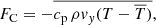
The solution obtained with the well-balanced scheme (along with some not well-balanced solutions, to be discussed below) is illustrated in Fig. 3. Convective roll-ups develop that persist as time evolves (panels a and b), closely resembling results by H84, their Fig. 4. Vertical time averaged profiles of FR, FC, and FK (green lines in panels d to f) are equally in line with H84. The radiative flux accounts for around 80% of the total flux in both cases. This value is to be expected for m = 1, while for m < 1 the convective flux will become more important and flow structures will be less smooth (see Brandenburg et al. 2005). In the mildly stratified case, energy transport via convection accounts for the remaining 20% of the total energy flux. In the strongly stratified case, the convective flux in addition compensates for the downward directed kinetic flux. Also shown in Fig. 3 are vertical time averaged profiles of the root mean square velocity, vrms. The quantity is clearly dominated by the horizontal branches of the convective motion. As such, vrms mirrors the overall shift of the convective roll-ups toward the lower boundary of the slab for χ = 21 as compared to χ = 1.5. The same dependence was reported in H84.
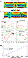 |
Fig. 3. Test case following H84. Typical flow patterns for χ = 1.5 and χ = 21 are shown in panels a and b, respectively, in (dimensionless) absolute velocity (color coded) with velocity arrows superimposed. Horizontally averaged vertical profiles of vrms, convective (FC), kinetic (FK), and radiative (FR) fluxes are given in panels c–f. Colors denote solutions obtained with the well-balanced scheme for χ = 1.5 (dark green) and χ = 21 (light green), with the well-balanced scheme but central differences for SE and χ = 21 (yellow), and with the standard scheme for χ = 21 (red). Solid lines are time averages, dashed lines are temporal variability (±1 standard deviation, where distinguishable from the mean). Panel g: time integrated gain of energy via SE if the scheme is not well balanced in energy (red dashed and blue solid) or if the standard scheme (purple dashed and cyan solid) is used for χ = 1.5 (dashed lines) and χ = 21 (solid lines, scaled by a factor of 30). |
To demonstrate the importance of the well-balanced scheme, we repeated each test case but relaxed the well-balanced properties of the scheme. The resulting, purely numerical energy gain via SE is illustrated in Fig. 3, panel g). The energy gain is found to be more severe for χ = 21 than for χ = 1.5 (by more than a factor of 30) and also more severe for the standard scheme than for the scheme that is well-balanced in SM but not in SE (more than a factor of 10). For χ = 21 and the standard scheme, the time integrated energy gain equals the total gas energy E of the slab after only about 1000 τs. The solution adjusts such that the temperature gradient steepens close to the top of the slab (not shown) and the excess energy gained is radiated via FR. This excess in FR near the top boundary is clearly visible in Fig. 3, panel f, yellow and red curves, showing the χ = 21 case. In the interior of the slab, FR remains unchanged whereas FC and FK both increase, as does vrms. If the standard scheme is used, the damage to the solution is particularly severe. Vertical profiles for χ = 21 (red lines in Fig. 3, panels c–f) now deviate substantially from the well-balanced solution, with strong temporal variability in the case of FC and FK. The latter is in line with the 2D flow field no longer being quasi-stationary: convective plumes move and occasionally the up-draft and down-draft branch approach so closely that convection collapses and re-forms.
3.2.3. 2D flows with low viscosity or high Rayleigh number
We repeated both 2D test cases to highlight two limiting cases that are well-documented in the literature and are of potential interest in the context of stellar convection modeling: low viscosity and high Rayleigh number (e.g., Muthsam et al. 1995; Brandenburg et al. 2005; Goluskin et al. 2014; van der Poel et al. 2014).
Setting μ = 0, we no longer observe quasi-stationary convection but intermittent, bursty convection. Figure 4, illustrates the situation for the χ = 1.5 case (with a Rayleigh number of 1.24 × 10⁵, K = 1.4 × 10⁻² and for a domain size of 8 instead of 4, which, however, has no effect). Strong horizontal or zonal flows prevail for most of the time (panel a), interrupted by occasional, short phases dominated by convective roll-ups (panel b). A similar behavior is reported by van der Poel et al. (2014). Going to much higher Rayleigh numbers while keeping σ = 1, the convective roll-ups permanently vanish in favor of zonal flow. A discussion of the underlying mechanisms may be found in Goluskin et al. (2014). Once a strong horizontal flow component starts developing, it hinders the organization of convection in the vertical direction. Stress-free boundaries, which are otherwise well-suited to model part of a stratified flow (e.g., Hossain & Mullan 1993), promote the occurrence of the phenomenon (e.g., Goluskin et al. 2014; van der Poel et al. 2014). We note that numerical viscosity is still present in all of the above flows, but it is apparently too small to prevent the occurrence of zonal flows. While zonal flows are widely reported in the context of compressible or Rayleigh–Bénard convection in 2D or quasi 2D for specific categories of flows (in particular for flows featuring high Rayleigh number, small viscosity, and stress-free boundaries), there exist to our knowledge no reports of zonal flows in truly 3D situations (Muthsam et al. 1995; Goluskin et al. 2014; van der Poel et al. 2014; Anders & Brown 2017).
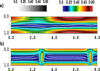 |
Fig. 4. Test case in 2D, following H84, for χ = 1.5 with μ = 0, K = 1.4 × 10⁻², and a Rayleigh number of 1.24 × 10⁵. The flow alters between long zonal-flow phases (panel a) and intermittent, convective burst phases (panel b). Absolute velocity is color coded, velocity arrows are overplotted in gray shadings. |
3.2.4. 3D simulation
We repeat the χ = 1.5 and χ = 21 setups in 3D to demonstrate that our algorithm works in 3D and to highlight some differences between 2D and 3D compressible convection (e.g., Muthsam et al. 1995; Ludwig & Nordlund 2000; Arnett et al. 2007; Mocák et al. 2009; Garaud & Brummell 2015). We use three 3D domains that have identical x- and y- extent as in Sect. 3.2.2 but differ in their z-extent: a “half bar” (z-extend 0.5), a “bar” domain (z-extent 1), and a “square” domain (z-extent 4). Gravity points along the y-axis. Discretization is as in 2D, that is, an extent of 1 is covered by 40 cells. We slightly perturb the velocity in the initialization to trigger convection but tested that this does not affect the results.
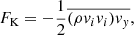
Aspects of the settled solutions for χ = 21 are illustrated in Fig. 5. From the velocity fields it can be seen that the half bar domain (panel a) settles into a very similar state to 2D. This organization remains stable over time. In the bar domain (panel b), the coherence of the 2D flow pattern already tends to be lost. Horizontal velocities near the top boundary and near the updraft (to the left in the figure) are no longer aligned with each other. The updraft region occasionally splits in two. In the square domain (panel c) the solution does not organize at all. Updrafts and downdrafts form and disappear, potentially moving around in between. A limitation on the geometrical degrees of freedom thus seems crucial for the organization of convection into steady roll-ups, at least in this particular test case. The relevant energy fluxes in the vertical direction, FR and FC, averaged horizontally and over time, (Fig. 5, panels e–g) change as well as. In particular, the convective flux FC peaks at lower values as one goes from 2D over half bar to bar to square. At the same time, the time variability (dashed lines in the figure) decreases. The root mean square velocity close to the top and bottom boundary of the slab decreases as the geometrical freedom increases from 2D to half bar, bar, and square. Differences are most pronounced between 2D and half bar on the one hand, and bar and square on the other hand.
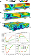 |
Fig. 5. Convective H84 slabs in 3D. Shown are the flow field (absolute dimensionless velocity color coded) for χ = 21 on domains half bar, bar and square (panels a–c), as well as vertical flux profiles (time averages, solid, and one standard deviation, dashed) for vrms, FC, FK, and FR (panels d–g). Discretization is 40 cells per interval [0, 1]. |
The χ = 1.5 case shows qualitatively the same behavior, but differences as one goes from 2D to square domain are generally less pronounced.
4. Application to the young sun
As a last test case we move to a more complicated and astrophysically more relevant situation: the model of a partially convective young sun. The test aims at demonstrating that the methods introduced work beyond comparatively simple test cases. In the absence of any analytical solution of the problem, we benchmark our results against corresponding, published simulations with the code MUSIC (Viallet et al. 2011, 2013, 2016; Goffrey et al. 2017). Our physical setup, to be detailed below, follows the one used in these studies. The section does not aim at a detailed physical comparison of the solutions obtained by MUSIC and A-MaZe, which is beyond the scope of the present paper and a topic of future studies.
4.1. Definition of the problem
We consider a model of a convective young sun with mass Mstar = 1 M⊙ and radius Rstar = 3 R⊙ at an age of a few Myr. We use the same realistic stellar, tabulated EoS p = p(ρ, e) (or, equivalently, T = T(ρ, e)) as in Pratt et al. (2016; see references therein). Inversion of the EoS is done numerically. Heat transfer is nonlinear and the heat conduction K(T) is, within the diffusion approximation for radiative transfer, given by the approximation
 (28)
(28)
where σ is the Stefan–Boltzmann constant and κ is the tabulated Rosseland opacity of the gas (Iglesias & Rogers 1996; Ferguson et al. 2005). The explicit viscosity μ is assumed to be zero, as the actual physical value is much smaller than the numerical viscosity. We use the same 1D initial model as used in Pratt et al. (2016). The gravitational potential ϕ is taken from the 1D simulations and is kept fixed in time. The average Mach number of the problem ranges from around 0.001 in the bulk of the convective zone to about 0.01 close to surface (see also Viallet et al. 2016).
We perform five simulations that differ in their resolution, geometry, and dimensionality. Four simulations use an axi-symmetric geometry, on grids of 642, 1282, 2562 and 5122. One simulation uses a 3D computational mesh of 643. A uniform mapping as in Sect. 3.1.2 is used: (x, y)→(r, θ) in the 2D axi-symmetric case and (x, y, z)→(r, θ, φ) in the 3D case with uniform grid spacing. In the radial direction and in units of stellar radius Rstar, the computational domain extends from Rmin = 0.21 to Rmax = 0.94 (“Low 3” case in Pratt et al. 2016), thereby comprising both, the convective envelope and parts of the radiative core. The domain extends from 0.2π to 0.8π in polar angle θ (and in azimuth angle φ in 3D).
Boundary conditions are periodic in angular directions. The slight dependence of the ghost cell volume for meridional directions (between a few percent and fractions of a percent, depending on resolution) is neglected, yet the fluxes at the periodic boundaries respect the conservative scheme. In radial direction, we set the mass fluxes at the domain boundary to zero (stress free for tangential velocities, reflecting for radial velocities), retain only the pressure term for the momentum fluxes (to ascertain well-balance), and prescribe fixed (radiative) energy fluxes taken from the initial 1D profile: 1.28 × 1032 ergs s−1 at the inner boundary and 8.91 × 1033 ergs s−1 at the outer boundary, which are then both scaled according to the fraction of the full sphere contained in the simulation domain. The luminosity L at the top and bottom of the domain is taken from the initial 1D profile. We note that more energy is radiated at the outer boundary than enters through the inner boundary, in line with the young sun being slowly contracting. To sustain a reasonable temperature profile close to the top boundary, despite our rather coarse numerical grid, we apply Newtonian cooling (Dobler et al. 2006; Viallet et al. 2011).
4.2. Axi-symmetric simulations
An illustration of the fully developed convection in the form of 2D velocity maps is given in Fig. 6 for the resolutions 2562 and 5122, comparable to cases “Low” and “Hi” in Pratt et al. (2016). The separation of the radiative core from the convective envelope is clearly apparent (transition to predominantly white color), at the same radial distance for both resolutions shown. Structures appear overall finer in the 5122 resolution case than in the 2562 case, as expected. The difference is particularly apparent when looking at the up- and down-drafts (colored in red and blue). Velocities tend to reach higher peak values in the 5122 case and are generally higher closer to the upper boundary.
The bottom panel of Fig. 6 roughly corresponds to Fig. 5, left panel, in Pratt et al. (2016). Comparing the two figures, they indeed look similar. In both figures, the separation between the radiative core and the convective envelope is located at about 1/3 of the radius shown. The up- and down-drafts appear rather more fine-grained and slightly more elongated in Fig. 6 than in Pratt et al. (2016).
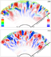 |
Fig. 6. Quasi-stationary convective structure of the young sun on the mesh 2562 (top panel) and 5122 (bottom panel). Shown is radial velocity (color coded, from blue, at −3000 m s−1 downward, to red, at +3000 m s−1 upward) with velocity arrows (rainbow colors according to magnitude, linear from 0 to 104 m s−1) after about 107 s (for comparison with Fig. 7). Color coding is the same in both panels. The domain extends in radial direction from 0.21 to 0.94 in units of Rstar, and from 0.2π to 0.8π in meridional direction. |
Convection in the A-MaZe simulations is overall more vigorous than in the MUSIC simulations, in terms of total kinetic energy or also with regard to vrms, both shown in Fig. 7. The total kinetic energy in the A-MaZe simulations is comparable for all resolutions, but systematically exceeds the value in MUSIC by roughly an order of magnitude. Turning from the total kinetic energy to the radial dependence of vrms, some more facets emerge. In the convection zone, vrms is larger in A-MaZe than in MUSIC (Fig. 7, middle panels). More specifically, both codes produce a comparable vrms close to the boundary between the radiative and the convective zone. But while in MUSIC there is little net increase of vrms with radius within the convective zone, vrms increases by about one order of magnitude in A-MaZe. Out to about 0.8 Rstar, the radial and tangential component of vrms increase in concert, reaching values somewhat above ∼1000 m s−1 (Fig. 7, bottom panels). Meanwhile, in MUSIC vrms reaches only ∼250 m s−1, yet again tangential velocities dominate for large radii. The difference also impacts the convective turnover time, which is often used as a characteristic time scale: the overall larger radial velocities in A-MaZe result in an overall shorter convective turnover time compared to MUSIC. At yet larger radial scales, beyond 0.8 Rstar, a large part of vrms in A-MaZe is contained in tangential velocities along the stellar surface. In the radiative zone, by contrast, A-MaZe yields robustly lower vrms than MUSIC (Fig. 7, middle panels).
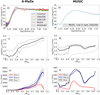 |
Fig. 7. Axi-symmetric young sun simulations, 2D, with A-MaZe (left panels, 2562 mesh unless otherwise stated) and MUSIC (right panels, “Low 3” case in Pratt et al. 2016). Shown are the total kinetic energy in the domain, scaled to a full spherical layer (0 ≤ θ ≤ π, 0 ≤ φ ≤ 2π, 0.21 ≤ R ≤ 0.94), as function of time (different resolutions color coded for A-MaZe, shifted in time such as to ramp up simultaneously), as well as radial profiles of volume-weighted vrms and its decomposition into radial and tangential component (middle and bottom panels, solid lines give time averages, dotted lines indicate the range) after convection has become quasi-stationary. The black long-dashed line (middle right panel) shows the convective velocity calculated within Mixing Length Theory formalism. We note that the y-axes in panels e and f are different. |
In summary, the above findings suggest qualitative agreement between A-MaZe and MUSIC, enhancing overall confidence in the results obtained by both codes. Yet quantitative differences exists. A detailed analysis of the underlying causes is beyond the scope of this paper. The analysis performed with MUSIC in Pratt et al. (2016) highlights the sensitivity of convective velocities to boundary conditions, extension of the radial domain and resolution, easily yielding a factor 5 difference between results based on different setups. Algorithmic differences may also contribute. On a more general level, the low Mach number limit of the compressible Euler (or Navier–Stokes) equations remains challenging, despite much progress in terms of physical understanding and numerical handling (e.g Guillard & Viozat 1999; Dellacherie 2010; Guillard & Nkonga 2017; Avgerinos et al. 2019). From this perspective, the differences documented here provide a basis for further numerical and physical progress.
4.3. 3D simulations
The results from the 3D simulation are illustrated in Fig. 8, at a time when convection has become quasi-stationary. The goal of these simulations is not the physical study of the young sun. The grid of 643 is too coarse to reasonably resolve numerous relevant physical structures, such as the strong temperature and density gradients characterising the near-surface layers. The purpose is rather to illustrate that the well-balanced scheme can cope with the application, despite coarse resolution and more complicated physics, notably in terms of EoS.
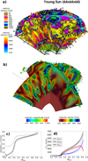 |
Fig. 8. Young sun simulation in 3D, 643 mesh. Panel a: surfaces of constant velocity along with velocity arrows. Panel b: slices along the equator and perpendicular to the equator. Shown is velocity magnitude (color coded) along with velocity arrows (arrows color coded according to velocity magnitude). Bottom panels: radial profiles of vrms (panel c, logarithmic scale) and of vrms split into radial and tangential components (panel d, total vrms also shown). Solid lines show time averages, the range (minimum to maximum) is indicted by dotted lines. |
Pockets of high-velocity material are visible in the top panel of Fig. 8, in cyan, blue, and green colors. The separation of the convective and the radiative zone is visible in Fig. 8, middle panel, as the transition to uniformly reddish colors. Also clearly visible in the same panel are numerous up- and down-drafts, some of the latter penetrating into the radiative zone. Across the transition from the convective to the radiative zone, vrms drops by a factor between ten to hundred, as can be taken from the bottom panels in Fig. 8. Radial profiles of vrms are qualitatively similar to their 2D counterparts (see Fig. 7). Also similar is the dominance of the tangential component for vrms for radii larger than about 0.8 Rstar, roughly the same radius as in the 2D simulations. The kinetic energy of the 3D 643 simulation is comparable to that in the 2562 and 5122 simulations in 2D (Fig. 7, top left panel). We take the above as an indication that our well-balanced implementation works equally well in both, 2D and 3D.
5. Discussion
In the following, we want to put the well-balanced extension to A-MaZe somewhat more into context. We will argue at the same time that the well-balanced extension, despite or because of its simplicity, makes A-MaZe a valuable tool for the numerical investigation of multidimensional stellar convection, especially in concert with other codes.
We noted already in Sect. 1 that there exist various approaches to cope with a gravitational field, be it external or due to self-gravity. With our choice of algorithm and its concrete implementation, we compromised on accuracy (second order in space in our implementation) and generality (stationary potential) in favor of simplicity and efficiency, both with regard to coding and execution time. The algorithm is compact and self-contained so that it can be implemented within an existing scheme or framework without difficulty. Additionally, the extension of the scheme to higher order accuracy for the non-hydrostatic part of the problem (p1 in Sect. 2.3.1) is straightforward. Going beyond second order for the hydrostatic reconstruction (p0 in Sect. 2.3.1) is more complex. The underlying assumption of ϕ being piece-wise linear is exactly fulfilled in the tests of Sect. 3, but only up to truncation errors in the case of the young sun, Sect. 4. In real application cases, the solution thus is potentially vulnerable again to too coarse meshes. However, this may not be a too severe restriction. In many astrophysical applications, ϕ varies more slowly and smoothly as a function of space and time than other physics of interest. A computational mesh fit for the latter is thus likely fine enough to somewhat mitigate the second order only reconstruction of p0 in practical applications. Issues potentially also exist in multi-dimensions if the gravitational force is not aligned with a coordinate axis, although practical applications do not appear to be severely impacted by this (see KM16 for a discussion). For the tests and applications of interest here, the restriction to a time-constant gravitational potential is not an issue. We see no principle obstacle as to why our approach should not be extendable to cases where ϕ is time dependent. In fact, KM16 present in their paper a corresponding test case, a toy model of a core-collapse supernova. It then would be interesting to compare the source term based approach presented here and a pure flux formulation as e.g., in Jiang et al. (2013).
Further advantages of the scheme exist beyond the previously mentioned simplicity and efficacy. The approach used here does not make any assumption on the thermal equilibrium, does not rely on a fixed mesh size, and allows for any time integration scheme, explicit or implicit (see KM16). Also, our cell-centered finite-volume scheme lends itself more easily to adaptive meshes than do staggered grids. The latter is potentially of interest in the context of our envisaged applications to stellar convection. In such applications, it may be desirable to have higher resolution at large stellar radii, toward the stellar surface, or also in the vicinity of ionization edges further inward. Finally, we have demonstrated in Sect. 4 that the current implementation, without adaptive grids, is useful for studying stellar convection: sufficiently long, physical integration times are possible despite explicit time stepping, and results are qualitatively comparable to MUSIC results. Associated integration times cannot be compared as the simulations were run on different machines. Comparisons of integration times for MUSIC alone may be found in Viallet et al. (2013; explicit versus previous implicit solver) and Viallet et al. (2016; previous versus current implicit solver).
Multidimensional studies of the interior dynamics of stars, from core to atmosphere, are still not common place and pose multiple, non-trivial challenges for numerical simulations. To ascertain the physical robustness of simulation results it is then advantageous to study the same situation with different simulation codes. This overarching idea resulted in the two codes MUSIC (Viallet et al. 2011, 2013, 2016) and the well-balanced hydro code within the A-MaZe tool-kit presented here. Similarities between both codes are, briefly, that they simulate hydrodynamic convection in stellar interiors in 2D and 3D for a realistic EoS. Major differences between A-MaZe and MUSIC concern the grid (cell-centered versus staggered) or the time integration (explicit versus implicit).
The differences between the two codes translate into different code-dependent strengths and weaknesses. The present paper demonstrates that both codes are basically fit to simulate stellar convection, thereby opening the possibility to duplicate at least some simulations or part thereof with both codes. Arriving at similar physical results with both codes greatly strengthens their credibility. Likewise, qualitative or quantitative difference point the way to where further improvement is needed in terms of numerics and physics.
6. Summary and conclusions
We equipped the multi-scale, multi-physics numerical tool-kit A-MaZe with a well-balanced algorithm that balances both, momentum and energy of a flow in the presence of a static gravitational field. The balancing with regard to energy is less of a topic in literature than the momentum balance, at least if the equations are formulated with source terms and not as a conservation law for the total energy of the gas, that is, internal plus kinetic plus gravitational energy.
A series of tests are presented that demonstrate the capabilities of our implementation, even at low resolution. An initially static configuration can be maintained to machine precision, even for a spherical setup on a Cartesian mesh. A quasi-stationary convective situation can be simulated without net gain or loss of energy despite strong local up-drafts and down-drafts. If a not (fully) well-balanced scheme is used, a substantial and steady energy gain on purely numerical grounds is shown to occur that affects the solution. The convection test is further used to exemplify differences between 2D and 3D convection, including the occurrence of zonal flows in 2D convection. Application of our code to a young sun in 2D and 3D, comprising an inner radiative and an outer convective part, completes our tests. Simulation results show reasonable agreement with published results.
With A-MaZe and MUSIC we now have two largely independent codes within our collaboration, with which to study multidimensional stellar convection or also simpler setups of compressible convection, like the ones used here primarily for code testing. Being able to repeat selected simulations or parts thereof with different codes promotes credibility of the obtained numerical results in case they are reasonably similar, or points the way to necessary physical or numerical improvements in case of substantial disagreement. The present work may also provide a direction of travel to defining benchmark cases for stellar convection beyond the usual Rayleigh–Bénard convection test cases, which would be useful for the rest of the community interested in the study of compressible convection.
Acknowledgments
We acknowledge support from the European Research Council through grants ERC-AdG No. 320478-TOFU and 787361-COBOM. This work was also partly supported by a Science and Technology Facilities Council Consolidated Grant (ST/R000395/1). RW and DF acknowledge support from the French National Program for High Energies PNHE. RW and DF are also grateful for the hospitality and fruitful discussion with the colleagues, in particular Professor Keh-Ming Shyue, of the Center for Theoretical Sciences, Mathematical Division at National Taiwan University where part of this work has been made. Dr. Jean M. Favre from the Swiss Supercompute Center (CSCS) we thank for sharing his profound knowledge on visualization and data analysis. An anonymous referee we thank for most constructive comments. Simulations have been performed at the Pôle Scientifique de Modélisation Numérique (PSMN), and at centers of the Grand Equipement National de Calcul Intensif (GENCI) under grant number A0310406960. We acknowledge the steady support of the staff at these two centers.
References
- Anders, E. H., & Brown, B. P. 2017, Phys. Rev. Fluids, 2, 083501 [NASA ADS] [CrossRef] [Google Scholar]
- Arnett, D., Meakin, C., & Young, P. A. 2007, in Convection in Astrophysics, eds. F. Kupka, I. Roxburgh, & K. L. Chan, IAU Symp., 239, 247 [NASA ADS] [Google Scholar]
- Arnett, W. D., Meakin, C., Viallet, M., et al. 2015, ApJ, 809, 30 [NASA ADS] [CrossRef] [Google Scholar]
- Avgerinos, S., Bernard, F., Iollo, A., & Russo, G. 2019, J. Comput. Phys., 393, 278 [NASA ADS] [CrossRef] [Google Scholar]
- Baraffe, I., Pratt, J., Goffrey, T., et al. 2017, ApJ, 845, L6 [NASA ADS] [CrossRef] [Google Scholar]
- Berberich, P., Chandrashekar, P., & Klingenberg, C. 2017, in Hyperbolic Problems: Theory, Numeric and Applications, Springer Proceedings in Mathematics and Statistics of the International Conference [Google Scholar]
- Berger, M. J., & Colella, P. 1989, J. Comput. Phys., 82, 64 [NASA ADS] [CrossRef] [Google Scholar]
- Berger, M. J., & Oliger, J. 1984, J. Comput. Phys., 53, 484 [NASA ADS] [CrossRef] [MathSciNet] [Google Scholar]
- Brandenburg, A., Chan, K. L., Nordlund, Å., & Stein, R. F. 2005, Astron. Nachr., 326, 681 [NASA ADS] [CrossRef] [Google Scholar]
- Calhoun, D. A., Helzel, C., & Leveque, R. J. 2008, SIAM Rev., 50, 723 [CrossRef] [Google Scholar]
- Cargo, P., & LeRoux, A. Y. 1994, Mathematique, 318, 73 [Google Scholar]
- Chandrashekar, P., & Klingenberg, C. 2015, SIAM J. Sci. Comput., 37, B382 [Google Scholar]
- Colella, P., & Glaz, H. M. 1985, J. Comput. Phys., 59, 264 [NASA ADS] [CrossRef] [Google Scholar]
- Couch, S. M., & Ott, C. D. 2013, ApJ, 778, L7 [NASA ADS] [CrossRef] [Google Scholar]
- Dellacherie, S. 2010, J. Comput. Phys., 229, 978 [CrossRef] [Google Scholar]
- Desveaux, V., Zenk, M., Berthon, C., & Klingenberg, C. 2016, Int. J. Numer. Methods Fluids, 81, 104 [NASA ADS] [CrossRef] [Google Scholar]
- Dobler, W., Stix, M., & Brandenburg, A. 2006, ApJ, 638, 336 [NASA ADS] [CrossRef] [Google Scholar]
- Ferguson, J. W., Alexander, D. R., Allard, F., et al. 2005, ApJ, 623, 585 [NASA ADS] [CrossRef] [Google Scholar]
- Folini, D., & Walder, R. 1999, in Wolf-Rayet Phenomena in Massive Stars and Starburst Galaxies, eds. K. A. van der Hucht, G. Koenigsberger, & P. R. J. Eenens, IAU Symp., 193, 352 [NASA ADS] [Google Scholar]
- Folini, D., & Walder, R. 2000, Ap&SS, 274, 189 [NASA ADS] [CrossRef] [Google Scholar]
- Folini, D., & Walder, R. 2006, A&A, 459, 1 [NASA ADS] [CrossRef] [EDP Sciences] [Google Scholar]
- Folini, D., Walder, R., Psarros, M., & Desboeufs, A. 2003, in Stellar Atmosphere Modeling, eds. I. Hubeny, D. Mihalas, & K. Werner, ASP Conf. Ser., 288, 433 [NASA ADS] [Google Scholar]
- Folini, D., Heyvaerts, J., & Walder, R. 2004, A&A, 414, 559 [NASA ADS] [CrossRef] [EDP Sciences] [Google Scholar]
- Folini, D., Walder, R., & Favre, J. M. 2014, A&A, 562, A112 [NASA ADS] [CrossRef] [EDP Sciences] [Google Scholar]
- Garaud, P., & Brummell, N. 2015, ApJ, 815, 42 [NASA ADS] [CrossRef] [Google Scholar]
- Georgy, C., Walder, R., Folini, D., et al. 2013, A&A, 559, A69 [NASA ADS] [CrossRef] [EDP Sciences] [Google Scholar]
- Geroux, C., Baraffe, I., Viallet, M., et al. 2016, A&A, 588, A85 [NASA ADS] [CrossRef] [EDP Sciences] [Google Scholar]
- Goffrey, T., Pratt, J., Viallet, M., et al. 2017, A&A, 600, A7 [NASA ADS] [CrossRef] [EDP Sciences] [Google Scholar]
- Goluskin, D., Johnston, H., Flierl, G. R., & Spiegel, E. A. 2014, J. Fluid Mechanics, 759, 360 [NASA ADS] [CrossRef] [Google Scholar]
- Gottlieb, S., Shu, C.-W., & Tadmor, E. 2001, SIAM Rev., 43, 89 [NASA ADS] [CrossRef] [MathSciNet] [Google Scholar]
- Greenberg, J. M., & Leroux, A. Y. 1996, SIAM J. Numer. Anal., 33, 1 [Google Scholar]
- Guillard, H., & Nkonga, B. 2017, in Handbook of Numerical Analysis, eds. R. Abgrall, & C. W. Shu (Elsevier), 18, 203 [Google Scholar]
- Guillard, H., & Viozat, C. 1999, Comput. Fluids, 28, 63 [Google Scholar]
- Hossain, M., & Mullan, D. J. 1993, ApJ, 416, 733 [NASA ADS] [CrossRef] [Google Scholar]
- Hurlburt, N. E., Toomre, J., & Massaguer, J. M. 1984, ApJ, 282, 557 [NASA ADS] [CrossRef] [Google Scholar]
- Iglesias, C. A., & Rogers, F. J. 1996, ApJ, 464, 943 [NASA ADS] [CrossRef] [Google Scholar]
- Jiang, Y.-F., Belyaev, M., Goodman, J., & Stone, J. M. 2013, New Astron., 19, 48 [NASA ADS] [CrossRef] [Google Scholar]
- Käppeli, R., & Mishra, S. 2014, J. Comput. Phys., 259, 199 [NASA ADS] [CrossRef] [Google Scholar]
- Käppeli, R., & Mishra, S. 2016, A&A, 587, A94 [NASA ADS] [CrossRef] [EDP Sciences] [Google Scholar]
- Kifonidis, K., & Müller, E. 2012, A&A, 544, A47 [NASA ADS] [CrossRef] [EDP Sciences] [Google Scholar]
- Kippenhahn, R., & Weigert, A. 1990, Stellar Structure and Evolution (Berlin: Springer), 192 [Google Scholar]
- LeVeque, R. J. 1998, J. Comput. Phys., 146, 346 [NASA ADS] [CrossRef] [MathSciNet] [Google Scholar]
- Ludwig, H. G., & Nordlund, A. 2000, in Astrophys. Space Sci. Lib., eds. K. S. Cheng, H. F. Chau, K. L. Chan, & K. C. Leung, 254, 37 [NASA ADS] [CrossRef] [Google Scholar]
- Melzani, M., Winisdoerffer, C., Walder, R., et al. 2013, A&A, 558, A133 [NASA ADS] [CrossRef] [EDP Sciences] [Google Scholar]
- Melzani, M., Walder, R., Folini, D., Winisdoerffer, C., & Favre, J. M. 2014a, A&A, 570, A111 [NASA ADS] [CrossRef] [EDP Sciences] [Google Scholar]
- Melzani, M., Walder, R., Folini, D., Winisdoerffer, C., & Favre, J. M. 2014b, A&A, 570, A112 [NASA ADS] [CrossRef] [EDP Sciences] [Google Scholar]
- Mocák, M., Müller, E., Weiss, A., & Kifonidis, K. 2009, A&A, 501, 659 [NASA ADS] [CrossRef] [EDP Sciences] [Google Scholar]
- Müller, B., Viallet, M., Heger, A., & Janka, H.-T. 2016, ApJ, 833, 124 [NASA ADS] [CrossRef] [Google Scholar]
- Müller, B., Melson, T., Heger, A., & Janka, H.-T. 2017, MNRAS, 472, 491 [NASA ADS] [CrossRef] [Google Scholar]
- Muthsam, H. J., Goeb, W., Kupka, F., Liebich, W., & Zoechling, J. 1995, A&A, 293, 127 [Google Scholar]
- Noelle, S., Xing, Y., & Shu, C.-W. 2009, High Order Well-balanced Schemes,, 24 (Napoli, Italy: Seconda Universita di Napoli) [Google Scholar]
- Nussbaumer, H., & Walder, R. 1993, A&A, 278, 209 [NASA ADS] [Google Scholar]
- Pratt, J., Baraffe, I., Goffrey, T., et al. 2016, A&A, 593, A121 [NASA ADS] [CrossRef] [EDP Sciences] [Google Scholar]
- Pratt, J., Baraffe, I., Goffrey, T., et al. 2017, A&A, 604, A125 [NASA ADS] [CrossRef] [EDP Sciences] [Google Scholar]
- Shu, C.-W., & Osher, S. 1988, J. Comput. Phys., 77, 439 [Google Scholar]
- Toro, E. F., Spruce, M., & Speares, W. 1994, Shock Waves, 4, 25 [NASA ADS] [CrossRef] [EDP Sciences] [Google Scholar]
- Touma, R., Koley, U., & Klingenberg, C. 2016, SIAM J. Sci. Comput., 38, B773 [Google Scholar]
- van der Poel, E. P., Ostilla-Mónico, R., Verzicco, R., & Lohse, D. 2014, Phys. Rev. E, 90, 013017 [NASA ADS] [CrossRef] [Google Scholar]
- Viallet, M., Baraffe, I., & Walder, R. 2011, A&A, 531, A86 [NASA ADS] [CrossRef] [EDP Sciences] [Google Scholar]
- Viallet, M., Baraffe, I., & Walder, R. 2013, A&A, 555, A81 [NASA ADS] [CrossRef] [EDP Sciences] [Google Scholar]
- Viallet, M., Goffrey, T., Baraffe, I., et al. 2016, A&A, 586, A153 [NASA ADS] [CrossRef] [EDP Sciences] [Google Scholar]
- Walder, R., & Folini, D. 2000, in Thermal and Ionization Aspects of Flows from Hot Stars, eds. H. Lamers, & A. Sapar, ASP Conf. Ser., 204, 281 [NASA ADS] [Google Scholar]
- Walder, R., Folini, D., & Shore, S. N. 2008, A&A, 484, L9 [NASA ADS] [CrossRef] [EDP Sciences] [Google Scholar]
- Walder, R., Melzani, M., Folini, D., Winisdoerffer, C., & Favre, J. M. 2014, in 8th International Conference of Numerical Modeling of Space Plasma Flows (ASTRONUM 2013), eds. N. V. Pogorelov, E. Audit, & G. P. Zank, ASP Conf. Ser., 488, 141 [NASA ADS] [Google Scholar]
- Wang, W., Shu, C.-W., Yee, H. C., & Sjögreen, B. 2009, J. Comput. Phys., 228, 6682 [NASA ADS] [CrossRef] [Google Scholar]
- Xing, Y., & Shu, C.-W. 2013, J. Sci. Comput., 54, 645 [Google Scholar]
All Figures
|
Fig. 1. Total mass in 1D hydrostatic slab, normalized by the initial mass (M(t)/M(t = 0), y-axis), as function of time (x-axis, in τs), integrated with the standard scheme, using either historical (dashed lines) or free-float (solid lines) boundary conditions and different meshes (colors; number of grid cells). The well-balanced scheme maintains M(t)/M(t = 0) = 1 to machine precision in all cases. |
| In the text | |
|
Fig. 2. Lane–Emden test case, preservation of initially static configuration. Top panel: using the standard scheme, a convection like velocity field develops. Shown is absolute velocity (from purple to white; sound speed ranging from 0.76 to 1.39) with velocity arrows (rainbow colored according to magnitude) for the axi-symmetric 2562 mesh after 300 τs. Bottom panel: using the well-balanced scheme, an initially static polytrope on a 3D Cartesian mesh (1283, star in a box) is preserved to machine precision. Shown are iso-surfaces in density after 300 τs. They remain perfectly spherical despite the Cartesian grid, because velocities remain zero to machine precision, thanks to the well-balanced scheme. |
| In the text | |
|
Fig. 3. Test case following H84. Typical flow patterns for χ = 1.5 and χ = 21 are shown in panels a and b, respectively, in (dimensionless) absolute velocity (color coded) with velocity arrows superimposed. Horizontally averaged vertical profiles of vrms, convective (FC), kinetic (FK), and radiative (FR) fluxes are given in panels c–f. Colors denote solutions obtained with the well-balanced scheme for χ = 1.5 (dark green) and χ = 21 (light green), with the well-balanced scheme but central differences for SE and χ = 21 (yellow), and with the standard scheme for χ = 21 (red). Solid lines are time averages, dashed lines are temporal variability (±1 standard deviation, where distinguishable from the mean). Panel g: time integrated gain of energy via SE if the scheme is not well balanced in energy (red dashed and blue solid) or if the standard scheme (purple dashed and cyan solid) is used for χ = 1.5 (dashed lines) and χ = 21 (solid lines, scaled by a factor of 30). |
| In the text | |
|
Fig. 4. Test case in 2D, following H84, for χ = 1.5 with μ = 0, K = 1.4 × 10⁻², and a Rayleigh number of 1.24 × 10⁵. The flow alters between long zonal-flow phases (panel a) and intermittent, convective burst phases (panel b). Absolute velocity is color coded, velocity arrows are overplotted in gray shadings. |
| In the text | |
|
Fig. 5. Convective H84 slabs in 3D. Shown are the flow field (absolute dimensionless velocity color coded) for χ = 21 on domains half bar, bar and square (panels a–c), as well as vertical flux profiles (time averages, solid, and one standard deviation, dashed) for vrms, FC, FK, and FR (panels d–g). Discretization is 40 cells per interval [0, 1]. |
| In the text | |
|
Fig. 6. Quasi-stationary convective structure of the young sun on the mesh 2562 (top panel) and 5122 (bottom panel). Shown is radial velocity (color coded, from blue, at −3000 m s−1 downward, to red, at +3000 m s−1 upward) with velocity arrows (rainbow colors according to magnitude, linear from 0 to 104 m s−1) after about 107 s (for comparison with Fig. 7). Color coding is the same in both panels. The domain extends in radial direction from 0.21 to 0.94 in units of Rstar, and from 0.2π to 0.8π in meridional direction. |
| In the text | |
|
Fig. 7. Axi-symmetric young sun simulations, 2D, with A-MaZe (left panels, 2562 mesh unless otherwise stated) and MUSIC (right panels, “Low 3” case in Pratt et al. 2016). Shown are the total kinetic energy in the domain, scaled to a full spherical layer (0 ≤ θ ≤ π, 0 ≤ φ ≤ 2π, 0.21 ≤ R ≤ 0.94), as function of time (different resolutions color coded for A-MaZe, shifted in time such as to ramp up simultaneously), as well as radial profiles of volume-weighted vrms and its decomposition into radial and tangential component (middle and bottom panels, solid lines give time averages, dotted lines indicate the range) after convection has become quasi-stationary. The black long-dashed line (middle right panel) shows the convective velocity calculated within Mixing Length Theory formalism. We note that the y-axes in panels e and f are different. |
| In the text | |
|
Fig. 8. Young sun simulation in 3D, 643 mesh. Panel a: surfaces of constant velocity along with velocity arrows. Panel b: slices along the equator and perpendicular to the equator. Shown is velocity magnitude (color coded) along with velocity arrows (arrows color coded according to velocity magnitude). Bottom panels: radial profiles of vrms (panel c, logarithmic scale) and of vrms split into radial and tangential components (panel d, total vrms also shown). Solid lines show time averages, the range (minimum to maximum) is indicted by dotted lines. |
| In the text | |
Current usage metrics show cumulative count of Article Views (full-text article views including HTML views, PDF and ePub downloads, according to the available data) and Abstracts Views on Vision4Press platform.
Data correspond to usage on the plateform after 2015. The current usage metrics is available 48-96 hours after online publication and is updated daily on week days.
Initial download of the metrics may take a while.