Fossil field decay due to nonlinear tides in massive binaries

J. Vidal; D. Cébron; A. ud-Doula; E. Alecian

doi:10.1051/0004-6361/201935658

Home

All issues

Volume 629 (September 2019)

A&A, 629 (2019) A142

Full HTML

Free Access

Issue		A&A Volume 629, September 2019


Article Number		A142
Number of page(s)		27
Section		Stellar structure and evolution
DOI		https://doi.org/10.1051/0004-6361/201935658
Published online		19 September 2019

A&A 629, A142 (2019)

Fossil field decay due to nonlinear tides in massive binaries

J. Vidal¹^,2, D. Cébron², A. ud-Doula³ and E. Alecian⁴

¹ Department of Applied Mathematics, School of Mathematics, University of Leeds, Leeds LS2 9JT, UK
e-mail: j.n.vidal@leeds.ac.uk
² Université Grenoble Alpes, CNRS, ISTerre, 38000 Grenoble, France
³ Penn State Scranton, 120 Ridge View Drive, Dunmore, PA 18512, USA
⁴ Université Grenoble Alpes, CNRS, IPAG, 38000 Grenoble, France

Received: 10 April 2019
Accepted: 5 August 2019

Abstract

Context. Surface magnetic fields have been detected in 5–10% of isolated massive stars, hosting outer radiative envelopes. They are often thought to have a fossil origin, resulting from the stellar formation phase. Yet, magnetic massive stars are scarcer in (close) short-period binaries, as reported by the BinaMIcS (Binarity and Magnetic Interaction in various classes of Stars) Collaboration.

Aims. Different physical conditions in the molecular clouds giving birth to isolated stars and binaries are commonly invoked. In addition, we propose that the observed lower magnetic incidence in close binaries may be due to nonlinear tides. Indeed, close binaries are probably prone to tidal instability, a fluid instability growing upon the equilibrium tidal flow via nonlinear effects. Yet, stratified effects have hitherto been largely overlooked.

Methods. We theoretically and numerically investigate tidal instability in rapidly rotating, stably stratified fluids permeated by magnetic fields. We use the short-wavelength stability method to propose a comprehensive (local) theory of tidal instability at the linear onset, discussing damping effects. Then, we propose a mixing-length theory for the mixing generated by tidal instability in the nonlinear regime. We successfully assess our theoretical predictions against proof-of-concept, direct numerical simulations. Finally, we compare our predictions with the observations of short-period, double-lined spectroscopic binary systems.

Results. Using new analytical results, cross-validated by a direct integration of the stability equations, we show that tidal instability can be generated by nonlinear couplings of inertia-gravity waves with the equilibrium tidal flow in short-period massive binaries, even against the Joule diffusion. In the nonlinear regime, a fossil magnetic field can be dissipated by the turbulent magnetic diffusion induced by the saturated tidal flows.

Conclusions. We predict that the turbulent Joule diffusion of fossil fields would occur in a few million years for several short-period massive binaries. Therefore, turbulent tidal flows could explain the observed dearth of some short-period magnetic binaries.

Key words: hydrodynamics / instabilities / waves / stars: magnetic field / stars: massive

© ESO 2019

1. Introduction

The magnetism of massive stars has sparked the interest of astronomers for a long time (Babcock 1958). More recently, large spectropolarimetric surveys of these stars have been undertaken (Hubrig et al. 2014; Wade et al. 2015; Grunhut et al. 2016). They have detected surface magnetic fields in 5–10% of pre-main sequence and main-sequence massive stars (e.g. Alecian et al. 2019; Mathys 2017). In addition, a magnetic dichotomy has been evidenced between the strong magnetism of chemically peculiar A/B stars (e.g. Auriere et al. 2007; Sikora et al. 2018) and the ultra-weak magnetism of Vega-like stars (Lignieres et al. 2009; Petit et al. 2010, 2011; Blazère et al. 2016). The origin of these fields is unclear. According to stellar evolution theory, massive stars host thick outer radiative envelopes, which are stably stratified in density. These envelopes are often assumed to be motionless in standard stellar models (e.g. Kippenhahn et al. 1990). This severely challenges the classical dynamo mechanism (Parker 1979), which requires internal turbulent motions (for instance that is convection in low-mass stars). Some dynamo mechanisms have been proposed, such as relying on the convection of the innermost convective core (Brun et al. 2005; Featherstone et al. 2009) generating magnetic flux tubes rising buoyantly towards the surface (MacGregor & Cassinelli 2003; MacDonald & Mullan 2004), on differentially rotating flows (Spruit 1999, 2002; Braithwaite 2006; Jouve et al. 2015) or on baroclinic flows (Simitev & Busse 2017). However, the relevance of these mechanisms remains elusive and debated.

The most accepted assumption is that magnetic fields in massive stars have a fossil origin (Borra et al. 1982; Moss 2001), because they appear relatively stable over the observational period. The fields would be shaped in the stellar formation phase and survive into later stages of stellar evolution. The fossil theory is now well supported by the existence of magnetic configurations stable enough to survive over a stellar lifetime (Braithwaite & Spruit 2004; Braithwaite & Nordlund 2006; Reisenegger 2009; Duez & Mathis 2010; Duez et al. 2010; Akgün et al. 2013). Hence, the fossil theory may provide a unifying explanation for the magnetism of intermediate-mass stars (Braithwaite & Spruit 2017). However, the fossil hypothesis still suffers from several weaknesses. In particular, we may naively expect all massive stars to exhibit surface magnetic fields. This is not consistent with the observations (e.g. Alecian et al. 2019; Mathys 2017). Moreover, the theory does not convincingly explain the observed magnetic bi-modality (e.g. Auriere et al. 2007). To solve these issues, different physical conditions in the star-forming regions are usually invoked (e.g. Commerçon et al. 2010, 2011).

An efficient way to assess this hypothesis is to survey close binaries. Although the formation of binaries is not well understood, we can reasonably assume that the two binary components were formed together, under similar physical conditions. Then, observing magnetic fields in the two components of a (short-period) binary system would provide constraints to disentangle initial condition effects from other possible physical effects. The BinaMIcS (Binarity and Magnetic Interaction in various classes of Stars) Collaboration (Alecian et al. 2014a, 2019) surveyed short-period massive binaries, aiming at providing new constraints on the magnetic properties of massive stars. About 170 short-period, double-lined spectroscopic binary binary systems on the main-sequence have been analysed by the BinaMIcS Collaboration (Alecian et al., in prep.). They have typical orbital periods of T_orb ≤ 20 days and a separation distance between the two components of D ≤ 1 au.

A magnetic incidence of about 1.5% has been measured in the BinaMIcS sample. This is much lower than what is typically found in isolated hot stars (see above). Therefore, radiative stars in short-period binary systems are apparently much less frequently magnetic than in isolated systems. This confirms the general trend observed in other studies, dedicated to intermediate-mass A-type stars (e.g. Carrier et al. 2002; Mathys 2017). It also extends it to hotter and more massive stars. Note that magnetic fields have been mostly observed only in one of the two components of the close binaries (Alecian et al. 2019), with a notable exception in the ϵ Lupi system (Shultz et al. 2015). If initial conditions were solely responsible for the presence of a fossil field, then we would naively expect fossil fields in the two components of a magnetic binary. This is clearly not a general trend. Thus, these puzzling observations defy the theories that are commonly invoked. They lead to scientific questions such as the following: is it due to formation processes (Commerçon et al. 2011; Schneider et al. 2016), that exclude more magnetic fields in binaries than in single stars? Or is there any other mechanism in close binaries, responsible for relatively quick dissipation of magnetic fields?

An alternative scenario is to invoke mixing in radiative envelopes, that may dissipate the pervading fossil fields dynamically. Identifying mixing sources in radiative stars is a long standing issue (see the review in Zahn 2008), because mixing also affects the transports of chemical elements and of angular momentum. Shear-driven turbulence, induced by the (expected) differential rotation of radiative envelopes (e.g. Goldreich & Schubert 1967; Rieutord 2006), has been largely investigated (e.g. Zahn 1974; Mathis et al. 2004, 2018).

A more efficient mixing in short-period stellar binaries may be provided by tides. Indeed, short-periods binaries are strongly deformed (e.g. Chandrasekhar 1969; Lai et al. 1993). Tides proceed in two steps. First, they generate a quasi-hydrostatic tidal bulge, known as the equilibrium tidal velocity field (Zahn 1966; Remus et al. 2012). This leads to angular momentum exchange between the orbital and spinning motions. Second, they induce dynamical tides (e.g. Zahn 1975; Rieutord & Valdettaro 2010), that is waves propagating here within the radiative regions. Radiative envelopes support the propagation of many waves that are continuously emitted by various mechanisms (e.g. Gastine & Dintrans 2008a,b; Mathis et al. 2014; Edelmann et al. 2019). Among them, internal gravity waves (Dintrans et al. 1999; Mirouh et al. 2016) do induce mixing processes in radiative regions (Schatzman 1993; Rogers & McElwaine 2017).

However, the aforementioned tidal effects are only linear processes. They are certainly relevant for the weak tides observed in the solar system and in extra-solar planets (Ogilvie 2009). Yet, they may be inefficient to modify fossil fields on their own. Moreover, nonlinear effects can significantly modify the outcome of the tidal response, and thereby the influence of tides on fossil fields. Indeed, the equilibrium tidal flow can be unstable against tidal instability in stars (e.g. Rieutord 2004; Le Bars et al. 2010; Barker & Lithwick 2013a,b; Clausen & Tilgner 2014; Barker et al. 2016; Barker 2016; Vidal & Cébron 2017; Vidal et al. 2018). This fluid instability is the astrophysical version of the generic elliptical instability, which affects all rotating fluids with elliptically deformed streamlines (Bayly 1986; Pierrehumbert 1986; Waleffe 1990; Gledzer & Ponomarev 1992; Le Dizès 2000). The underlying physical mechanism is nonlinear triadic resonances between two waves and the background elliptical velocity (Kerswell 2002). Hence, in stellar interiors, the origin of tidal instability is a resonance between rotational waves and the underlying strain field responsible for the elliptic deformation, that is the equilibrium tidal flow. The nonlinear saturation of tidal instability can exhibit a wide variety of nonlinear states in homogeneous fluids, such as space-filling small-scale turbulence (Le Reun et al. 2017; Le Reun & Favier 2019) or even global mixing (Grannan et al. 2016; Vidal et al. 2018). Interestingly, Clausen & Tilgner (2014) investigated the influence of compressibility on the stability limits of tidal instability in stars or planets. They showed that fluid compressibility has almost no effect on the onset of tidal instability.

Yet, the fate of tidal instability in stratified fluid interiors is poorly known. On the one hand, theoretical studies have shown that an axial density stratification, aligned with the spin angular velocity, has stabilising effects (Miyazaki & Fukumoto 1991, 1992). Moreover, in the equatorial region, radial stratification can either increase or decrease the growth rate of the instability (Kerswell 1993a; Le Bars & Le Dizès 2006; Cébron et al. 2013). On the other hand, three-dimensional numerical simulations suggest that tidal instability is largely unaffected in stratified interiors, for a wide range of stratification (Cébron et al. 2010; Vidal et al. 2018). Therefore, a consistent global picture of tidal instability in stably stratified interiors is highly desirable. Indeed, this is a prerequisite to assess the astrophysical relevance of tidal instability for the stellar mixing in close massive binaries.

The present study has a twofold purpose. First, we aim to propose a predictive global theory of tidal instability in idealised stratified interiors. Such a theory should accurately predict the onset of instability, reconciling within a single framework previous theoretical analyses (Miyazaki & Fukumoto 1992; Miyazaki 1993; Kerswell 1993a; Le Bars & Le Dizès 2006) and numerical studies (Cébron et al. 2010; Le Reun et al. 2018; Vidal et al. 2018). Then, asymptotic predictions for the (nonlinear) tidal mixing, as found numerically in Vidal et al. (2018), must be obtained to carry out the astrophysical extrapolation. Second, we aim to propose a new physical scenario of turbulent Joule diffusion of fossil fields, compatible with the observed lower magnetic incidence in short-period massive binaries as analysed by the BinaMIcS Collaboration (Alecian et al., in prep.). The paper is organised as follows. In Sect. 2, we present the idealised model. In Sect. 3, we investigate the linear regime of tidal instability in stratified interiors. In Sect. 4, we develop a mixing-length theory of the (turbulent) tidal mixing, which is compared with proof-of-concept simulations. Then, we attempt to propose a novel scenario for close binaries in Sect. 5, which is applied to short-period binary systems analysed by the BinaMIcS Collaboration. Finally, we end the paper with a conclusion in Sect. 6 and outline some perspectives.

2. Formulation of the problem

2.1. Assumptions

The full astrophysical problem is rather complex. Hence, we consider an idealised model, for which numerical simulations can be conducted and compared with theory. We describe here the main assumptions, as they will be used throughout the paper. Our model retains the essential features to study tidal instability: rotation, stratification, magnetic fields and a tidally deformed geometry.

We consider a primary self-gravitating body of mass M₁ and volume 𝒱, filled with an electrically conducting and rotating fluid. Radiative fluid envelopes are expected to undergo differential rotation (Goldreich & Schubert 1967), for instance provided by the contraction occurring during the pre-main-sequence phase or baroclinic torques (Busse 1981, 1982; Rieutord 2006). However, differential rotation tends to be smoothed out by hydromagnetic effects (e.g. Moss 1992). In particular, differential rotation may sustain magneto-rotational instability, ultimately leading a state of solid-body rotation (Arlt et al. 2003; Rüdiger et al. 2013, 2015) on a few Alfvén timescales (Jouve et al. 2015). Consequently, we assume that the radiative envelope is uniformly rotating.

Then, the primary is orbited by a companion star of mass M₂. We investigate here only short-period, non-coalescing binaries. Due to the interplay between rotation and gravitational effects, the shape of each binary component departs from the spherical geometry. We do not seek here the mutual tidal interactions between the primary and the secondary. Indeed, at the leading order, the primary (or the secondary) is a triaxial ellipsoid in solid-body rotation (e.g. Chandrasekhar 1969; Lai et al. 1993), as obtained by modelling the other component by a point-mass companion. Therefore, for the sake of simplicity, we treat the secondary as a point mass for the orbital dynamics (e.g. Hut 1981, 1982).

The secondary rises an equilibrium tide (Zahn 1966; Remus et al. 2012) on the fluid primary, with a typical equatorial amplitude denoted β₀. An initially eccentric binary system, with non-synchronised rotating components, evolves towards an orbital configuration characterised by a circular orbit and, ultimately, the system will be synchronised (Hut 1981, 1982). For weakly elliptic orbits, Nduka (1971) showed that the ellipsoidal distortion β₀ points toward the tidal companion at the leading order. Vidal & Cébron (2017) also showed that weak orbital eccentricities have little effects on the internal fluid dynamics of the primary (at the leading order in the eccentricity). Thus, we assume that the binary system is circularised (or weakly eccentric), with an equatorial bulge aligned with the orbital companion.

Then, we consider only the leading-order component of the tidal potential, associated with the asynchronous tides (Ogilvie 2014). The fluid spin and orbital angular velocities are coplanar and aligned in the inertial frame. Note that this is the expected equilibrium state of the system (e.g. Chandrasekhar 1969). The other tidal components, for instance obliquity tides, are mainly responsible for additional fluid instabilities that are superimposed on tidal instability (e.g. Kerswell 1993b). They can be neglected in a first attempt.

Within the fluid primary, diffusive effects appear at the second order for tidal instability, in the absence of significant surface diffusive effects at a free boundary (Rieutord 1992; Rieutord & Zahn 1997). Hence, we assume that the fluid has a uniform kinematic viscosity ν, a radiative (thermal) diffusivity κ_T (Kippenhahn et al. 1990) and a magnetic diffusivity η = 1/(μ₀σ), where σ is the electrical conductivity and μ₀ the magnetic permeability of free space. Finally, Clausen & Tilgner (2014) showed that compressibility has almost no effect on tidal instability. Therefore, we model density variations departing from the isentropic profile within the Boussinesq approximation (Spiegel & Veronis 1960).

2.2. Governing equations

The radiative star is modelled as a tidally deformed, uniformly rotating and stably stratified fluid domain in the Boussinesq approximation. The fluid domain, of typical density ρ_M = M₁/𝒱, is rotating at the angular velocity Ω_s in the inertial frame. The orbital configuration is illustrated in Fig. 1. The orbital angular velocity in the inertial frame is denoted Ω_orb 1_z, with Ω_orb ≠ Ω_s for a non-synchronised orbit. In the central frame, in which the boundary shape is stationary, the outer boundary ∂𝒱 of the fluid domain describes an ellipsoid (e.g. Chandrasekhar 1969; Lai et al. 1993). Its mathematical expression in Cartesian coordinates (x, y, z) is

$\begin{matrix} (\frac{x}{a})^{2} + (\frac{y}{b})^{2} + (\frac{z}{c})^{2} = 1, \end{matrix}$ $\begin{aligned} \left (\frac{x}{a}\right )^2 + \left (\frac{y}{b}\right )^2 + \left (\frac{z}{c}\right )^2 = 1, \end{aligned}$ (1)

where (a, b, c) are the semi-axes. The equatorial ellipticity is defined by β₀ = |a² − b²|/(a² + b²).

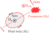Fig. 1.

Sketch of idealised orbital configuration between primary body of mass M₁ and secondary one of mass M₂. View from above in the inertial frame. Coplanar and aligned spin and orbital angular velocities [Ω_s, Ω_orb].

In the following, we work in dimensionless variables. To do so, we choose a typical radius R of the fluid domain as unit of length, $Ω_{s}^{- 1}$ $\Omega_\mathrm{s}^{-1}$ as a unit of time, $Ω_{s}^{2} R / (α_{T} g_{0})$ $\Omega_\mathrm{s}^2 R/(\alpha_{\rm T} {\it g}_0)$ as unit of the temperature with g₀ a typical value of the gravity field at the outer boundary and α_T the thermal expansion coefficient (at constant pressure). For the magnetic field, we choose $Ω_{s} R \sqrt{ρ_{M} μ_{0}}$ $\Omega_\mathrm{ s} R \sqrt{\rho_{\mathrm{M}} \mu_0}$ as typical unit. We also introduce the dimensionless orbital frequency Ω₀ = Ω_orb/Ω_s. The dimensionless variables are the velocity field v, the temperature field T, the magnetic field B and the gravity field g. They are written without ^*, to distinguish them from their dimensional counterparts [v^*, T^*, B^*, g^*]. The field variables, at the position r and time t, are governed in the rotating central frame by momentum, energy and induction equations. They read

$\begin{matrix} \frac{\partial v}{\partial t} = - (v \cdot \nabla) v - 2 Ω_{0} 1_{z} \times v - \nabla (P + P_{m}) + E k \nabla^{2} v \\ - T g + (B \cdot \nabla) B, \end{matrix}$ $\begin{aligned}&\frac{\partial \boldsymbol{v}}{\partial t} = - (\boldsymbol{v} \boldsymbol{\cdot } \nabla ) \, \boldsymbol{v} - 2 \Omega _0 \, \boldsymbol{1}_z \times \boldsymbol{v} -\nabla (P+P_{\rm m}) + Ek \, \boldsymbol{\nabla }^2 \boldsymbol{v} \nonumber \\&\qquad - T \boldsymbol{g} + (\boldsymbol{B} \cdot \nabla ) \, \boldsymbol{B}, \end{aligned}$ (2a)

$\begin{matrix} \frac{\partial T}{\partial t} = - (v \cdot \nabla) T + \frac{Ek}{\Pr} \nabla^{2} T + Q, \end{matrix}$ $\begin{aligned}&\frac{\partial T}{\partial t} = - (\boldsymbol{v} \boldsymbol{\cdot } \nabla ) \, T + \frac{Ek}{Pr} \nabla ^2 T + \mathcal{Q} , \end{aligned}$ (2b)

$\begin{matrix} \frac{\partial B}{\partial t} = \nabla \times (v \times B) + E m \nabla^{2} B, \end{matrix}$ $\begin{aligned}&\frac{\partial \boldsymbol{B}}{\partial t} = \boldsymbol{\nabla } \times (\boldsymbol{v} \times \boldsymbol{B}) + Em \, \boldsymbol{\nabla }^2 \boldsymbol{B}, \end{aligned}$ (2c)

$\begin{matrix} \nabla \cdot v = \nabla \cdot B = 0, \end{matrix}$ $\begin{aligned}&\boldsymbol{\nabla } \boldsymbol{\cdot } \boldsymbol{v} = \boldsymbol{\nabla } \boldsymbol{\cdot } \boldsymbol{B} = 0, \end{aligned}$ (2d)

with P the hydrostatic pressure (including centrifugal effects), P_m = |B|²/2 the magnetic pressure, 𝒬 a heat source term and g = −∇Φ₀ the (imposed) gravity field in the Boussinesq approximation. In governing Eqs. (2), we have introduced as dimensionless numbers the Ekman number Ek = ν/(Ω_sR²), the Prandtl number Pr = ν/κ_T, the magnetic Prandtl number Pm = ν/η and the magnetic Ekman number Em = Ek/Pm. Typical values are given in Table 1 for stellar interiors. The latter are characterised by weakly diffusive conditions (that is Ek, Ek/Pr, Ek/Pm ≪ 1). This regime will greatly simplify the analysis of tidal instability.

Table 1.

Typical values of dimensionless numbers for stellar interiors. CZ: stellar convective zones, e.g. in the Sun (Charbonneau 2014). RZ: (rapidly) rotating radiative zones (e.g. Rieutord 2006).

We do not directly solve full Eqs. (2). Indeed, a reference ellipsoidal state is always first established, on which tidal instability grows upon and nonlinearly saturates. We expand the field variables as perturbations (not necessarily small) around a steady reference ellipsoidal basic state [U₀, T₀](r) (detailed in Sect. 2.3). Thus, the dimensionless nonlinear governing equations for the perturbations [u, Θ](r, t) and the magnetic field B(r, t) are

$\begin{matrix} \frac{d u}{d t} + (u \cdot \nabla) u = - (u \cdot \nabla) U_{0} - 2 Ω_{0} 1_{z} \times u - \nabla (p + P_{m}) \\ + E k \nabla^{2} u - Θ g + (B \cdot \nabla) B, \end{matrix}$ $\begin{aligned}&\frac{\mathrm{d} \boldsymbol{u}}{\mathrm{d} t} + (\boldsymbol{u} {\cdot } \nabla ) \, \boldsymbol{u} = - (\boldsymbol{u} {\cdot } \nabla ) \, \boldsymbol{U}_0 - 2 \Omega _0 \, \boldsymbol{1}_z \, \times \boldsymbol{u} -\nabla (p + P_{\rm m})\nonumber \\&\quad \,\, + Ek \, \boldsymbol{\nabla }^2 \boldsymbol{u} - \Theta \boldsymbol{g} + (\boldsymbol{B}\boldsymbol{\cdot } \nabla ) \, \boldsymbol{B} , \end{aligned}$ (3a)

$\begin{matrix} \frac{d Θ}{d t} + (u \cdot \nabla) Θ = - (u \cdot \nabla) T_{0} + \frac{Ek}{\Pr} \nabla^{2} Θ, \end{matrix}$ $\begin{aligned}&\frac{\mathrm{d} \Theta }{\mathrm{d} t} + (\boldsymbol{u} {\cdot } \nabla ) \, \Theta = - (\boldsymbol{u} {\cdot } \nabla ) \, T_0 + \frac{Ek}{Pr} \nabla ^2 \Theta , \end{aligned}$ (3b)

$\begin{matrix} \frac{\partial B}{\partial t} + \nabla \times (B \times u) = \nabla \times (U_{0} \times B) + E m \nabla^{2} B, \end{matrix}$ $\begin{aligned}&\frac{\partial \boldsymbol{B}}{\partial t} + \boldsymbol{\nabla } \times (\boldsymbol{B} \times \boldsymbol{u} ) = \boldsymbol{\nabla } \times \left( \boldsymbol{U}_0 \times \boldsymbol{B} \right) + Em \, \boldsymbol{\nabla }^2 \boldsymbol{B}, \end{aligned}$ (3c)

$\begin{matrix} \nabla \cdot u = \nabla \cdot B = 0, B (r, t = 0) = B_{0} (r), \end{matrix}$ $\begin{aligned}&\boldsymbol{\nabla } \boldsymbol{\cdot } \boldsymbol{u} = \boldsymbol{\nabla } \boldsymbol{\cdot } \boldsymbol{B} = 0,\,\boldsymbol{B}(\boldsymbol{r},t=0) = \boldsymbol{B}_0(\boldsymbol{r}), \end{aligned}$ (3d)

with d/dt = ∂/∂t + (U₀⋅∇) the material derivative along the basic flow p the hydrodynamic pressure and B₀(r) the (initial) fossil field. For the proof-of-concept simulations introduced in Sect. 4, the equations will be supplemented by appropriate boundary conditions.

2.3. Reference ellipsoidal configuration

We consider a steady reference equilibrium state, for which isopycnals coincide with isopotentials of the gravitational potential Φ₀ (including centrifugal force, self-gravity and tides). This assumption is consistent with compressible models (Lai et al. 1993). Hence, we assume that the background temperature profile T₀(r) and the gravity field g, solutions of Eqs. (2a) and (2b), are in barotropic equilibrium (for a well-chosen 𝒬) such that g × (∇T₀)=0. We do not consider the baroclinic part, which is known to increase the growth rate of tidal instability in the equatorial plane (Kerswell 1993a; Le Bars & Le Dizès 2006). In the nonlinear regime, a baroclinic state would certainly sustain tidal turbulence in stellar interiors. However, we focus here on the less favourable configuration for the growth of tidal instability (that is barotropic stratification). This choice is also consistent with the assumed uniform rotation of the fluid. Indeed, baroclinic torques are known to sustain differential rotation (e.g. Busse 1981, 1982; Rieutord 2006). Moreover, considering barotropic stratification is a relevant assumption when the isopycnals move sufficiently fast to keep track of the rotating tidal potential (Le Reun et al. 2018). This situation is expected when stratification is large enough in amplitude compared with the differential rotation Ω_s − Ω_orb between the spin and the orbit.

To characterise the strength of stratification, we introduce the dimensional (local) Brunt–Väisälä frequency N in the reference state. In dimensional variables, the latter is defined by

$\begin{matrix} N^{2} = - α_{T} g^{*} \cdot \nabla T_{0}^{*} . \end{matrix}$ $\begin{aligned} N^2 = - \alpha _{\rm T} \, \boldsymbol{g}^* \boldsymbol{\cdot } \nabla T_0^*. \end{aligned}$ (4)

The fluid ellipsoid is assumed to be entirely stably stratified in density (N² > 0). The exact profiles in stellar interiors depend on the stellar internal processes. However, we want to compare analytical and numerical computations, which cannot be done for arbitrary profiles. Thus, we assume that the dimensionless total gravitational potential is quadratic, such that

$\begin{matrix} Φ_{0} = {(\frac{x}{a})}^{2} + {(\frac{y}{b})}^{2} + {(\frac{z}{c})}^{2} . \end{matrix}$ $\begin{aligned} \Phi _0 = \left(\frac{x}{a}\right)^2 + \left(\frac{{ y}}{b}\right)^2 + \left(\frac{z}{c}\right)^2. \end{aligned}$ (5)

Then, we consider the (dimensionless) reference temperature in barotropic equilibrium $T_{0} = (N_{0}^{2} / Ω_{s}^{2}) Φ_{0}$ $T_0 = (N^2_0/\Omega^2_\mathrm{s}) \, \Phi_0$ , with N₀ a typical value of the Brunt–Väisälä frequency at the outer boundary. For intermediate-mass stars with M₁ = 3 M_⊙ (where M_⊙ is the solar mass), a typical value is N₀ ∼ 10⁻³ s⁻¹ (e.g. Rieutord 2006), and typical values of $Ω_{s}^{- 1}$ $\Omega_\mathrm{s}^{-1}$ range between 1 and 100 days (Mathys 2017). This give the estimate 0 ≤ N₀/Ω_s ≤ 100 in radiative stars. Hence, a barotropic reference configuration is a reasonable starting assumption.

The ellipsoid is initially permeated by an fossil magnetic field B₀(r) (in dimensionless form). To measure its relative strength (with respect to rotation), we introduce the (dimensionless) Lehnert number (Lehnert 1954)

$\begin{matrix} L e = \frac{B_{0}^{*}}{Ω_{s} R \sqrt{ρ_{M} μ_{0}}}, \end{matrix}$ $\begin{aligned} Le = \frac{B_0^*}{\Omega _\mathrm{ s} R \sqrt{\rho _{\rm M} \mu _0}}, \end{aligned}$ (6)

where $B_{0}^{*}$ $ B_0^* $ is the typical (dimensional) strength of the fossil field. The Lehnert number is the ratio of the Alfvén and rotational velocities. When Le ≪ 1, the Coriolis force dominates the Lorentz force in momentum Eq. (2a). The regime Le ≪ 1 is encountered in many magnetic stars (Table 1). In the Sun, a typical value is Le ∼ 10⁻⁵ (Charbonneau 2014). For the scarce magnetic binaries which have been observed, the median field strength is $B_{0}^{*} \sim 1 kG$ $B_0^* \sim 1\,{\rm kG}$ (see also values in Table 4). This gives the typical values Le ≤ 10⁻⁵ − 10⁻⁴. Hence, we focus on the regime Le ≪ 1 in the following.

Finally, the orbital configuration drives the equilibrium tidal flow (e.g. Remus et al. 2012). For non-synchronised orbits (Ω₀ ≠ 1), its leading-order flow components in the central frame are (e.g. Cébron et al. 2012a; Vidal & Cébron 2017)

$\begin{matrix} U_{0} (r) = (1 - Ω_{0}) [- (1 + β_{0}) y 1_{x} + (1 - β_{0}) x 1_{y}] . \end{matrix}$ $\begin{aligned} \boldsymbol{U}_0(\boldsymbol{r}) = (1-\Omega _0) \left[-(1+\beta _0) { y} \, \boldsymbol{1}_x + (1-\beta _0)x \, \boldsymbol{1}_{ y} \right]. \end{aligned}$ (7)

with [1_x, 1_y, 1_z] the unit Cartesian vectors. This is an exact incompressible solution of hydrodynamic momentum Eq. (2a) without diffusion. Moreover, it satisfies the non-penetration condition U₀⋅1_n = 0 at the boundary ∂𝒱, with 1_n the unit outward normal vector. Note that basic flow (7) is not rigorously a solution in the presence of an arbitrary magnetic field. Yet, the large-scale poloidal and toroidal components of B₀(r) are unlikely to modify the equilibrium tidal flow in the weak field regime Le ≪ 1 as often assumed (e.g. Kerswell 1993a, 1994; Mizerski & Bajer 2011).

3. Onset of tidal instability

We present the stability analysis of tidal instability at the linear onset. First, we outline the general stability method in Sect. 3.1. In Sect. 3.2, we carry out an asymptotic analysis to get physical insight of the instability mechanism. The latter mechanism is compared and validated with the (numerical) solutions of the full stability equations in Sect. 3.3, without making any prior assumption. Finally, we discuss the (laminar) magnetic diffusive effects in Sect. 3.4.

3.1. Short-wavelength perturbations

In the absence of any driving mechanism, a fossil field B₀ slowly decays on the Ohmic diffusive timescale (Ω_s Ek/Pm)⁻¹. This time is larger than the typical lifetime of the least massive stars on the main-sequence (e.g. Braithwaite & Spruit 2017). However, Eqs. (3) support the propagation of several waves in rotating radiative interiors, characterised by Le ≪ 1 and N₀/Ω_s ≫ 1 (see Table 1). They can strongly modify the dynamical evolution of radiative envelopes. These waves are continuously emitted and, in the presence of tides, they can be nonlinearly coupled with the equilibrium tidal velocity field U₀ to sustain tidal instability. Tidal instability is intrinsically a local (small scale) instability (Kerswell 2002; Cébron et al. 2012a; Barker & Lithwick 2013a,b), but it also exists in global models (e.g. Kerswell 1993a; Grannan et al. 2016; Vidal et al. 2018). The global stability analysis is beyond the scope of the present study. However, in the diffusionless regime, three-dimensional global perturbations of small enough length scales are excited (e.g. Vidal & Cébron 2017), such that they are not affected by the boundary. Hence, we can advantageously investigate the growth of tidal instability in stellar interiors by performing a local stability analysis. In Appendix A, we have extended the general local stability theory to account for combined magnetic and buoyancy effects within the Boussinesq approximation.

We focus on the subsonic wave spectrum (low Mach number), made of MAC (Magneto-Archimedean-Coriolis) waves. Indeed, high-frequency sonic waves are not involved in tidal (elliptical) instability (Le Duc 2001), though they may be coupled with tides (e.g. in coalescing binary neutron stars, see Weinberg 2016). The properties of MAC waves have already been outlined elsewhere (e.g. Gubbins & Roberts 1987; Mathis & de Brye 2011; Sreenivasan & Narasimhan 2017). Note that they have global bounded counterparts, known as Magneto-Archimedean-Coriolis (MAC) modes. The global modes are briefly discussed in Appendix B. The wave spectrum is bounded from below by slow Magneto-Coriolis (MC) waves, sustained by the Lorentz and Coriolis forces with an angular frequency ω_i scaling as |ω_i| ∝ Le² (e.g. Malkus 1967; Labbé et al. 2015). The spectrum is bounded from above by internal gravity waves (modified by rotation), with an angular frequency |ω_i| ≤ N₀/Ω_s for strong stratification (Friedlander & Siegmann 1982a). In-between, the spectrum exhibits Coriolis waves (Greenspan 1968; Backus & Rieutord 2017) and inertial-gravity (or gravito-inertial) waves (e.g. Dintrans et al. 1999; Mirouh et al. 2016).

In the weak field limit Le ≪ 1, magnetic effects are negligible (at the leading order) on inertial waves (Schmitt 2010; Labbé et al. 2015) and gravito-inertial ones, as outlined in Appendix B. Moreover, only nonlinear couplings of inertial and gravito-inertial waves can trigger tidal instability with significant growth rates to overcome the leading-order diffusive effects (Kerswell 1993a, 1994), as we confirm in Appendix C. This behaviour is also supported by local simulations (Barker & Lithwick 2013a) and global dynamo numerical simulations in homogeneous (Cébron & Hollerbach 2014; Reddy et al. 2018) and stratified fluids (Vidal et al. 2018). They showed that even a dynamo magnetic field only barely modifies the hydrodynamic tidal flows. Therefore, we can consider only the hydrodynamic Boussinesq stability equations in relevant the weak field regime Le ≪ 1. The leading-order magnetic effect is the Joule diffusion. From the values given in Table 1, diffusive effects can be a priori neglected at the first order of the stability theory. We will confirm that this assumption is relevant by reintroducing them in Sect. 3.4.

We seek three-dimensional local perturbations, solution of linearised hydrodynamic Eqs. (3). To do so, we consider short-wavelength (WKB) perturbations (Lifschitz & Hameiri 1991; Friedlander & Vishik 1991). They are local (plane-wave) perturbations, barely sensitive to the ellipsoidal boundary ∂𝒱, advected along the fluid trajectories X(t) of U₀(r). Given basic tidal flow (7), the Eulerian three-dimensional perturbations are expressed as

$\begin{matrix} [u, Θ] (r, t) = [\hat{u}, \hat{Θ}] (r, t) exp (i k (t) \cdot r), | k (t) | = | k_{0} |, \end{matrix}$ $\begin{aligned}[ \boldsymbol{u}, \Theta ] (\boldsymbol{r},t) = [ \boldsymbol{\widehat{u}}, \widehat{\Theta } ] (\boldsymbol{r},t) \, \exp (\mathrm{i} \boldsymbol{k} (t) \boldsymbol{\cdot } \boldsymbol{r}), \ \, \ |\boldsymbol{k}(t)| = |\boldsymbol{k}_0|, \end{aligned}$ (8)

where k(t) is the local wave vector with the initial value k₀. The local stability equations are solved in Lagrangian formulation, yielding the following ordinary differential equations (in dimensionless form)

$\begin{matrix} \frac{D X}{D t} = U_{0} (X), X (0) = X_{0}, \end{matrix}$ $\begin{aligned}&\frac{\mathrm{D} \boldsymbol{X}}{\mathrm{D} t} = \boldsymbol{U}_0 (\boldsymbol{X}), \ \, \ \boldsymbol{X}(0) = \boldsymbol{X}_0, \end{aligned}$ (9a)

$\begin{matrix} \frac{D k}{D t} = - {(\nabla U_{0})}^{⊤} k, k (0) = k_{0}, \end{matrix}$ $\begin{aligned}&\frac{\mathrm{D} \boldsymbol{k}}{\mathrm{D} t} = - \left( \boldsymbol{\nabla } \boldsymbol{U}_0 \right)^\top \boldsymbol{k}, \ \, \ \boldsymbol{k}(0) = \boldsymbol{k}_0, \end{aligned}$ (9b)

$\begin{matrix} \frac{D \hat{u}}{D t} = [(\frac{2 k k^{T}}{{| k |}^{2}} - I) \nabla U_{0} + 2 (\frac{k k^{T}}{{| k |}^{2}} - I) Ω_{0} 1_{z} \times] \hat{u} \\ - \hat{Θ} (I - \frac{k k^{T}}{{| k |}^{2}}) g, \end{matrix}$ $\begin{aligned}&\frac{\mathrm{D} \boldsymbol{\widehat{u}}}{\mathrm{D} t} = \left[ \left( \frac{2\, \boldsymbol{k} \boldsymbol{k}^{T}}{|\boldsymbol{k}|^2} - \boldsymbol{I} \right) \boldsymbol{\nabla } \boldsymbol{U}_0 +2 \left( \frac{ \boldsymbol{k} \boldsymbol{k}^{T}}{|\boldsymbol{k}|^2}-\boldsymbol{I} \right) \Omega _{0} \, \boldsymbol{1}_z \times \right]\, \boldsymbol{\widehat{u}} \nonumber \\&\quad \quad \,\,\,- \widehat{\Theta } \left( \boldsymbol{I} -\frac{ \boldsymbol{k} \boldsymbol{k}^{T}}{|\boldsymbol{k}|^2} \right) \boldsymbol{g}, \end{aligned}$ (9c)

$\begin{matrix} \frac{D \hat{Θ}}{D t} = - (\hat{u} \cdot \nabla) T_{0}, \end{matrix}$ $\begin{aligned}&\frac{\mathrm{D} \widehat{\Theta }}{\mathrm{D} t} = - (\boldsymbol{\widehat{u}} \boldsymbol{\cdot } \nabla ) \, T_0 , \end{aligned}$ (9d)

with D/Dt the Lagrangian time derivative. The solenoidal condition $\hat{u} \cdot k = 0$ $\boldsymbol{\widehat{u}} \cdot \boldsymbol{k} = 0$ is satisfied as long as it holds at the initial time, that is $\hat{u} (0) \cdot k_{0} = 0$ $\boldsymbol{\widehat{u}} (0) \cdot \boldsymbol{k}_0 = 0$ in the Lagrangian description. Equations (9) do depend on the fluid trajectories X(t), because the gravity field g is spatially varying.

Equations (9) are ordinary differential equations along the Lagrangian trajectories X(t). They are also independent of the magnitude of k₀ in the diffusionless limit. We follow Le Dizès (2000), by restricting the initial wave vector to the unit spherical surface

$\begin{matrix} k_{0} = sin (θ_{0}) cos (ϕ_{0}) 1_{x} + sin (θ_{0}) sin (ϕ_{0}) 1_{y} + cos (θ_{0}) 1_{z}, \end{matrix}$ $\begin{aligned} \boldsymbol{k}_0 = \sin (\theta _0) \cos (\phi _0) \, \boldsymbol{1}_x + \sin (\theta _0) \sin (\phi _0) \, \boldsymbol{1}_{ y} + \cos (\theta _0) \, \boldsymbol{1}_z, \end{aligned}$ (10)

where ϕ₀ ∈ [0, 2π] is the longitude and θ₀ ∈ [0, π] is the colatitude between the spin axis 1_z and the wave vector k₀. In practice, Eqs. (9) are integrated from a range of wave vectors k₀ and initial positions X₀ within the reference ellipsoidal domain. The basic state is unstable against short-wavelength perturbations if

$\begin{matrix} lim_{t \to \infty} (| \hat{u} (t, X_{0}, k_{0}) | + | \hat{Θ} (t, X_{0}, k_{0}) |) = \infty . \end{matrix}$ $\begin{aligned} \lim \limits _{t\rightarrow \infty } \left( |\boldsymbol{\widehat{u}} (t, \boldsymbol{X}_0, \boldsymbol{k}_0)| + |\widehat{\Theta } (t, \boldsymbol{X}_0, \boldsymbol{k}_0)| \right) = \infty . \end{aligned}$ (11)

Then, we determine the maximum (diffusionless) growth rate σ as the fastest growing solution for all initial conditions, that is the largest Lyapunov exponent. This gives a sufficient condition for instability.

3.2. Asymptotic analysis

Equilibrium tidal flow (7) admits analytical periodic fluid trajectories X(t) and wave vectors k(t), solution of Eqs. (9a) and (9b). To get physical insight of the instability mechanism, we carry out an asymptotic analysis in the limit β₀ ≤ 1. We expand all quantities ( $X, k, \hat{u}, \hat{Θ}$ $\boldsymbol{X}, \boldsymbol{k}, \boldsymbol{\widehat{u}}, \widehat{\Theta}$ ) in successive powers of β₀ (see technical details in Le Dizès 2000).

3.2.1. Triadic (nonlinear) couplings

It has been recognised for a long time that tidal instability is a parametric instability in homogeneous (e.g. Bayly 1986; Waleffe 1990) and stratified fluids (e.g. Miyazaki & Fukumoto 1992; Miyazaki 1993). The instability is due to triadic interactions between pairs of waves that are coupled with the underlying tidal flow (7). At the leading asymptotic order (β₀ = 0), a necessary condition for a parametric tidal instability in rotating fluids is given by the resonance condition in the central frame (Kerswell 2002; Vidal & Cébron 2017)

$\begin{matrix} | ω_{i} - ω_{j} + δ | = 2 | 1 - Ω_{0} |, \end{matrix}$ $\begin{aligned} |\omega _i - \omega _j + \delta | = 2 \, |1-\Omega _0|, \end{aligned}$ (12)

where [ω_i, ω_j] are the angular frequencies of two free waves and δ a small detuning parameter, allowing for imperfect resonances (Kerswell 1993a; Le Dizès 2000; Lacaze et al. 2004; Vidal & Cébron 2017). The latter are due to either diffusive or topographic effects (δ → 0 for diffusionless fluids and weakly deformed spheres β₀ ≪ 1). Detuning effects are negligible in the astrophysical regime (almost diffusionless and with β₀ ≪ 1). Note that the case of synchronised orbits, characterised by Ω₀ = 1 (in average), is forbidden by condition (12). Synchronised orbits must be treated separately (see Appendix D).

Among the aforementioned resonances, sub-harmonic resonances are characterised by ω_i = −ω_j. Then, resonance condition (12) reduces (in the diffusionless regime) to

$\begin{matrix} | ω_{i} | = | 1 - Ω_{0} |, \end{matrix}$ $\begin{aligned} |\omega _i| = |1-\Omega _0|, \end{aligned}$ (13)

which is a necessary condition for sub-harmonic tidal instability. Sub-harmonic resonances have been found to be the most unstable in homogeneous fluids (Kerswell 1993a, 1994; Le Dizès 2000; Vidal & Cébron 2017), that is generating the largest growth rates.

We are now in a position to survey the possible nonlinear couplings of the different types of waves that can trigger tidal instability. The waves can be combined in several ways to satisfy the resonance condition in non-synchronised systems. For instance, from condition (13), tidal instability traditionally exists in the orbital range −1 ≤ Ω₀ ≤ 3 when it involves Coriolis waves (e.g. Craik 1989; Le Dizès 2000; Vidal & Cébron 2017). We investigate in depth the coupling of hydrodynamic waves, postponing the discussion of hydromagnetic waves (unimportant for the present problem) to Appendix C.

3.2.2. Hydrodynamic waves at the parametric resonance

The behaviour of tidal instability is intrinsically associated with the properties of the waves involved in the triadic resonances. The wave-like equation, introduced in Appendix B, is a mixed hyperbolic-elliptic partial differential equation. In the general case, a wave-like hyperbolic domain coexists with an elliptic domain, in which the waves are evanescent. At the leading asymptotic order β₀ = 0, the characteristic curve delimiting the two domains is (Friedlander & Siegmann 1982b)

$\begin{matrix} z^{2} + s^{2} ω_{i}^{2} / (ω_{i}^{2} - 4) = ω_{i}^{2} / {(N_{0} / Ω_{s})}^{2}, \end{matrix}$ $\begin{aligned} z^2 + s^2 \omega _i^2/ (\omega _i^2 - 4) = \omega _i^2/(N_0/\Omega _\mathrm{ s})^2, \end{aligned}$ (14)

with s the cylindrical radius. The hydrodynamic wave spectrum is divided in two main regimes. On the one hand, we have inertial waves modified by gravity, called inertial-gravity waves and denoted ℋ. They have hyperbolic turning surfaces given by Eq. (14). They are sub-divided in two families given by

$\begin{matrix} H_{1} : & {(N_{0} / Ω_{s})}^{2} < ω_{i}^{2} < 4, \end{matrix}$ $\begin{aligned} \mathcal{H} _1:&\ (N_0/\Omega _\mathrm{ s})^2 < \omega _i^2 < 4, \end{aligned}$ (15a)

$\begin{matrix} H_{2} : & 0 < ω_{i}^{2} < min [4, {(N_{0} / Ω_{s})}^{2}] . \end{matrix}$ $\begin{aligned} \mathcal{H} _2:&\ 0 < \omega _i^2 < \min \, [4, (N_0/\Omega _\mathrm{ s})^2]. \end{aligned}$ (15b)

On the other hand, we have gravity waves modified by rotation, called gravito-inertial waves and denoted ℰ. They have ellipsoidal turning surfaces given by Eq. (14). They are also divided in two families, characterised by

$\begin{matrix} E_{1} : & 4 < ω_{i}^{2} < {(N_{0} / Ω_{s})}^{2}, \end{matrix}$ $\begin{aligned} \mathcal{E} _1:&\ 4 < \omega _i^2 < (N_0/\Omega _\mathrm{ s})^2, \end{aligned}$ (16a)

$\begin{matrix} E_{2} : & max [4, {(N_{0} / Ω_{s})}^{2}] < ω_{i}^{2} < 4 + {(N_{0} / Ω_{s})}^{2} . \end{matrix}$ $\begin{aligned} \mathcal{E} _2:&\ \max \, [4, (N_0/\Omega _\mathrm{ s})^2] < \omega _i^2 < 4 + (N_0/\Omega _\mathrm{ s})^2. \end{aligned}$ (16b)

These properties are quite general, because Eq. (14) depends solely on the reference state. Therefore, both global modes (e.g. Dintrans et al. 1999) and local waves propagating upon this reference configuration exhibit this distinction.

The different families of waves satisfying sub-harmonic resonance condition (13) are illustrated in Fig. 2. This is the main result of the linear theory, as this provides a necessary (and sufficient, see below) condition for the existence of tidal instability (in both global and local models). Two kinds of tidal instability can be obtained, depending on the value of key parameter Ω₀. At the leading asymptotic order, we have obtained a general expression for sub-harmonic resonance condition (13) in the local theory, which can be written as

$\begin{matrix} {cos}^{2} (θ_{0}) & = \frac{\tilde{ω} + {\tilde{N}}_{0}^{2} r_{0}^{2} [({\tilde{N}}_{0}^{2} r_{0}^{2} - \tilde{ω}) {cos}^{2} α_{0} - cos (2 α_{0})]}{{\tilde{ω}}^{2} + {\tilde{N}}_{0}^{2} r_{0}^{2} [{\tilde{N}}_{0}^{2} r_{0}^{2} - 2 \tilde{ω} cos (2 α_{0})]} \\ + \frac{2 \sqrt{ω_{1} [\tilde{ω} (1 - {\tilde{N}}_{0}^{2} z_{0}^{2}) + {\tilde{N}}_{0}^{2} r_{0}^{2} - 1]}}{{\tilde{ω}}^{2} + {\tilde{N}}_{0}^{2} r_{0}^{2} [{\tilde{N}}_{0}^{2} r_{0}^{2} - 2 \tilde{ω} cos (2 α_{0})]}, \end{matrix}$ $\begin{aligned} \cos ^2 (\theta _0)&= \frac{\widetilde{\omega }+\widetilde{N}_0^2 r_0^2 \, [(\widetilde{N}_0^2 r_0^2 - \widetilde{\omega }) \cos ^2 \alpha _0 -\cos (2 \alpha _0)]}{\widetilde{\omega }^2+\widetilde{N}_0^2 r_0^2 \, [\widetilde{N}_0^2 r_0^2-2 \widetilde{\omega } \cos (2 \alpha _0)]} \nonumber \\&\qquad \qquad \; + \frac{2 \sqrt{\omega _1 \, [\widetilde{\omega } \, (1-\widetilde{N}_0^2 z_0^2)+\widetilde{N}_0^2 r_0^2 - 1]}}{\widetilde{\omega }^2+\widetilde{N}_0^2 r_0^2 \, [\widetilde{N}_0^2 r_0^2 - 2 \widetilde{\omega } \cos (2 \alpha _0)]}, \end{aligned}$ (17)

with the background rotation ${\tilde{Ω}}_{0} = Ω_{0} / (1 - Ω_{0})$ $\widetilde{\Omega}_0\,{=}\,\Omega_0/(1-\Omega_0)$ , ${\tilde{N}}_{0} = (N_{0} / Ω_{s}) / | 1 - Ω_{0} |$ $\widetilde{N}_0 = (N_0/\Omega_\mathrm{ s})/|1-\Omega_0|$ , $\tilde{ω} = 4 {(1 + {\tilde{Ω}}_{0})}^{2}$ $\widetilde{\omega}=4(1+\widetilde{\Omega}_0)^2$ , the initial position X₀ = (x₀, z₀)^⊤ = r₀ (sinα₀, cos α₀)^⊤ where r₀ is the initial radius and $ω_{1} = {\tilde{N}}_{0}^{4} r_{0}^{4} {cos}^{2} α_{0} {sin}^{2} α_{0}$ $\omega_1=\widetilde{N}_0^4 r_0^4 \cos^2 \alpha_0 \sin^2 \alpha_0$ . The associated wave-like domains and colatitude angles θ₀ are shown in Figs. 3 and 4.

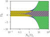Fig. 2.

Domains of existence of sub-harmonic resonances (13), as a function of Ω₀ = Ω_orb/Ω_s and N₀/Ω_s. In white regions, no waves can satisfy sub-harmonic resonance condition (13). Stars (yellow area): hyperbolic waves ℋ₁. Right slash (purple area): hyperbolic waves ℋ₂. Dots (green area): elliptic waves ℰ₁. Back slash (blue area): elliptic waves ℰ₂. The classical allowable region of tidal instability (for neutral fluids) is −1 ≤ Ω₀ < 3. wave-like domains [ℋ₁, ℋ₂] are illustrated in Fig. 3. Similarly, wave-like domains [ℰ₁, ℰ₂] are illustrated in Fig. 4.

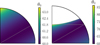Fig. 3.

Wave-like domains and colatitude θ₀ (degrees) for waves with hyperbolic turning surfaces ℋ satisfying sub-harmonic resonance condition (13). Left panel: ℋ₁ wave: Ω₀ = 0, N₀/Ω_s = 0.5. Right panel: ℋ₂ wave: Ω₀ = 0, N₀/Ω_s = 2. Dashed grey hyperbolic curve is given by Eq. (14). Tilted dashed grey line is the asymptotic curve given by cos θ₀ = |1 − Ω₀|/2. Waves at the sub-harmonic resonance disappear along the polar axis when z ≤ |1 − Ω₀|/(N₀/Ω_s).

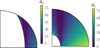Fig. 4.

Wave-like domains and colatitude θ₀ (degrees) for waves with ellipsoidal turning surface ℰ satisfying sub-harmonic resonance condition (13). Left panel: ℰ₁ wave: Ω₀ = 3.4, N₀/Ω_s = 2. Right panel: ℰ₂ wave: Ω₀ = 4, N₀/Ω_s = 10. Dashed grey ellipsoidal curve is given by Eq. (14). Vertical dashed grey line is the asymptotic curve given by $s = \sqrt{| 1 - Ω_{0} |^{2} - 4} / (N_{0} / Ω_{s})$ $s = \sqrt{|1-\Omega_0|^2 - 4}/(N_0/\Omega_\mathrm{ s})$ , where s is the cylindrical radius from the spin axis. Waves satisfying the sub-harmonic resonance condition disappear along the polar axis when z ≤ |1 − Ω₀|/(N₀/Ω_s).

The classical allowable range of the instability in homogeneous fluids is −1 ≤ Ω₀ ≤ 3 (Craik 1989; Le Dizès 2000). Within this range, the sub-harmonic condition involves only ℋ waves, as shown in Fig. 2. For neutral stratification (N₀ = 0), they are inertial waves ℋ₁, propagating in the whole fluid cavity (Friedlander & Siegmann 1982b). They have the colatitude angle at the sub-harmonic resonance (Le Dizès 2000)

$\begin{matrix} 2 cos (θ_{0}) = \frac{1}{1 + {\tilde{Ω}}_{0}} = 1 - Ω_{0} . \end{matrix}$ $\begin{aligned} 2\, \cos (\theta _0) = \frac{1}{1+\widetilde{\Omega }_0} = 1-\Omega _0. \end{aligned}$ (18)

This remains valid in weakly stratified fluids (that is N₀/Ω_s ≪ 1). Indeed, ℋ₁ waves are only slightly modified by buoyancy. They still propagate in the whole fluid domain, as shown in Fig. 3 (left panel). In addition, their colatitude angle θ₀ is slightly larger than the value predicted by formula (18) on the polar axis.

When N₀/Ω_s ≥ 1, ℋ₁ waves morph into ℋ₂ waves made of inertia-gravity waves. These waves are strongly modified by buoyancy. Their wave-like domain is confined between hyperboloids, as shown in Fig. 3 (right panel). Outside the hyperboloid volume, these waves at the sub-harmonic resonance are evanescent (in global models). The characteristic curve delimiting the wave-like and evanescent domains, given by Eq. (14), is hyperbolic. Along the rotation axis, local waves at the sub-harmonic resonance do not propagate in the evanescent regions for vertical positions z_c satisfying

$\begin{matrix} | z_{c} | \geq \frac{| 1 - Ω_{0} |}{N_{0} / Ω_{s}} \cdot \end{matrix}$ $\begin{aligned} |z_{\rm c}| \ge \frac{|1-\Omega _0|}{N_0/\Omega _\mathrm{ s}}\cdot \end{aligned}$ (19)

This shows that axial stratification has a stabilising effect.

This behaviour is responsible for an equatorial trapping of the waves in the other directions at the sub-harmonic resonance. Indeed, the hyperbolic wave-like domain, bounded by (14), converges towards the conical volume delimited by the asymptotic limit cos(θ_c)=|1 − Ω₀|/2 (Friedlander & Siegmann 1982b), where θ_c is the critical colatitude. This is exactly formula (18). Therefore, expression (18) also defines the position of the critical latitudes at which the waves at the sub-harmonic resonance have a group velocity orthogonal to the gravity field (here the radial direction at the leading order in β₀), that is a wave vector k ∝ g. Hence, these specific waves are insensitive to stratification. We emphasise that the presence of stratification does not alter the position of the critical latitudes (Friedlander & Siegmann 1982a,b). When |1 − Ω₀|→0, the waves at the sub-harmonic resonance are equatorially trapped according to formula (18).

The orbital range Ω₀ ≤ −1 and Ω₀ ≥ 3 is known as the forbidden zone. In this range, tidal instability must involve gravito-inertial waves ℰ for the sub-harmonic mechanism, whatever the strength of stratification. Indeed, Fig. 2 clearly shows that the waves at the sub-harmonic resonance depend only on the value of the orbital frequency Ω₀. When N₀/Ω_s ≤ 1, the sub-harmonic condition is never satisfied within this orbital range. Hence, no tidal instability is triggered.

However, gravito-inertial waves ℰ can be excited at the sub-harmonic resonance for strong stratification, typically N₀/Ω_s ≫ 1 when |Ω₀| increases. Their critical characteristic surfaces, given by Eq. (14), are ellipsoidal. On the one hand, ℰ₁ gravito-inertial waves are trapped in a region that does not encompass the polar axis, as shown in Fig. 4 (left panel). The minimum distance between the spin axis and the wave-like domain in the equatorial plane is given by (Friedlander & Siegmann 1982b)

$\begin{matrix} x_{c} = \frac{\sqrt{| 1 - Ω_{0} |^{2} - 4}}{N_{0} / Ω_{s}} \cdot \end{matrix}$ $\begin{aligned} x_{\rm c} = \frac{\sqrt{|1-\Omega _0|^2 - 4}}{N_0/\Omega _\mathrm{ s}}\cdot \end{aligned}$ (20)

Therefore, the thickness of the wave-like domain increases when the ratio N₀/Ω_s increases. On the other hand, ℰ₂ waves at the sub-harmonic resonance are gravito-inertial waves, trapped in a region that excludes the central part of the fluid (right panel of Fig. 4). Along the polar axis, these waves do not propagate when z is smaller than critical value (19). The size of wave-like domain increases when the ratio N₀/Ω_s increases. In the limit N₀/Ω_s → ∞, these waves become almost pure internal gravity waves, propagating in the whole fluid domain at the sub-harmonic resonance. This situation has been investigated numerically in local models (Le Reun et al. 2018), by assuming Ω_s = 0.

3.2.3. Asymptotic growth rate in the equatorial plane

At the next asymptotic order in β₀, we can obtain a concise explicit formula for the growth rate σ of tidal instability, valid in the equatorial plane z₀ = 0. Dispersion relation (17) gives, for α₀ = π/2 (after simplification),

$\begin{matrix} \sqrt{\tilde{ω} + {\tilde{N}}_{0}^{2} x_{0}^{2}} cos (θ_{0}) = \pm 1 \end{matrix}$ $\begin{aligned} \sqrt{\widetilde{\omega } + \widetilde{N}_0^2 x_0^2} \, \cos (\theta _0) = \pm 1 \end{aligned}$ (21)

with x₀ ≤ 1 the position of the initial trajectory X₀ in the equatorial plane. In the particular case Ω₀ = 0, Eq. (21) recovers Eq. (4.6) of Le Bars & Le Dizès (2006).

Several configurations are possible, depending on the parameters. On the one hand, the LHS of Eq. (21) is purely imaginary when $- {\tilde{N}}_{0}^{2} x_{0}^{2} > \tilde{ω}$ $-\widetilde{N}_0^2 x_0^2 > \widetilde{\omega}$ , when stratification is unstably stratified (with $N_{0}^{2} / Ω_{s}^{2} \leq 0$ $N_0^2/\Omega_\mathrm{s}^2 \leq 0$ . Then, a centrifugal instability grows upon the reference configuration, with a maximum (dimensionless) growth rate (e.g. Le Bars & Le Dizès 2006)

$\begin{matrix} \frac{σ}{| 1 - Ω_{0} |} = \sqrt{- {\tilde{N}}_{0}^{2} x_{0}^{2} - \tilde{ω}} . \end{matrix}$ $\begin{aligned} \frac{\sigma }{|1-\Omega _0|} = \sqrt{-\widetilde{N}_0^2 x_0^2 - \widetilde{\omega }}. \end{aligned}$ (22)

On the other hand, tidal instability is triggered when all terms in Eq. (21) are real. Hence, no sub-harmonic instability is possible when ${\tilde{N}}_{0}^{2} x_{0}^{2} < - 3 - 4 {\tilde{Ω}}_{0} (2 + {\tilde{Ω}}_{0})$ $\widetilde{N}_0^2 x_0^2 < -3 - 4\widetilde{\Omega}_0 \, (2+\widetilde{\Omega}_0)$ . This defines the forbidden zone of tidal instability in stably stratified fluids, at a given position x₀. For neutral fluids (N₀ = 0), we recover the classical allowable orbital range of tidal instability −1 ≤ Ω₀ ≤ 3. Outside this range, we find that waves can be involved in triadic resonances in stratified fluids. Thus, (sub-harmonic) tidal instability could be triggered in stratified fluids when Ω₀ ≤ −1 and Ω₀ ≥ 3 (range known as the forbidden zone in neutral fluids). Then, the dimensionless growth rate in the equatorial plane is

$\begin{matrix} \frac{σ}{| 1 - Ω_{0} |} = \frac{{(2 {\tilde{Ω}}_{0} + 3)}^{2}}{16 {(1 + {\tilde{Ω}}_{0})}^{2} + 4 {\tilde{N}}_{0}^{2} x_{0}^{2}} β_{0} . \end{matrix}$ $\begin{aligned} \frac{\sigma }{|1-\Omega _0|} = \frac{(2 \widetilde{\Omega }_0+3)^2}{16 \, (1+\widetilde{\Omega }_0)^2+4\widetilde{N}_0^2 x_0^2} \beta _0. \end{aligned}$ (23)

Hence, the growth rate σ is weakened by stratification when ${\tilde{N}}_{0}^{2} x_{0}^{2}$ $\widetilde{N}_0^2 x_0^2$ increases. This effect was already discussed in the conclusion of Le Bars & Le Dizès (2006). They found that elliptical equipotentials are stabilising contrary to circular equipotentials. However, in this former case, their equation slightly differs from Eq. (23). Actually, their formula is erroneous because we will confirm the validity of expression (23) by direct numerical integration of the local stability equations (see below). Note also that Eq. (23) does not recover Eq. (24) of Cébron et al. (2013), obtained in the limit of a buoyancy force of order β₀. In this limit, we recover their approximate formula (24) if we use their value for θ₀, artificially set to its hydrodynamic value $\tilde{ω} {cos}^{2} θ_{0} = 1$ $\widetilde{\omega} \cos^2 \theta_0=1$ instead of its exact value given by (21).

We show in Fig. 5 the maximum growth rate, computed from formula (23), for different orbital configurations Ω₀. Several points are worthy of comment. First, tidal instability is excited in the equatorial region when −1 ≤ Ω₀ ≤ 3 (in the diffusionless limit), that is in the classical orbital range of tidal instability (Le Dizès 2000). This mechanism occurs for any realistic value of N₀/Ω_s ≤ 100 (see Table 1). In this orbital range, the maximum growth rate is always obtained for neutral fluids (N₀ = 0), yielding the usual (dimensionless) growth rate (Le Dizès 2000)

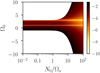$\begin{matrix} \frac{σ}{| 1 - Ω_{0} |} = \frac{{(2 {\tilde{Ω}}_{0} + 3)}^{2}}{16 {(1 + {\tilde{Ω}}_{0})}^{2}} β_{0} . \end{matrix}$ $\begin{aligned} \frac{\sigma }{|1-\Omega _0|} = \frac{(2 \widetilde{\Omega }_0+3)^2}{16 \, (1+\widetilde{\Omega }_0)^2} \beta _0. \end{aligned}$ (24)

Fig. 5.

Growth rate σ of tidal instability, predicted by formula (23) in equatorial plane (x₀ = 0.5, z₀ = 0), as a function of N₀/Ω_s and Ω₀. Colour bar shows the normalised ratio log₁₀(σ/β₀). White areas correspond to marginally stable areas. For neutral fluids, tidal instability is restricted to the allowable range −1 ≤ Ω₀ ≤ 3 when β₀ ≪ 1. When Ω₀ = 1 (horizontal white line), the basic state is synchronised (see Appendix D).

Second, outside the classical orbital range (in the forbidden zone), we unravel new tidal instabilities, triggered for large enough values of the Brunt–Väisälä frequency (N₀/Ω_s ≫ 1). Their growth rate can be larger than one in our dimensionless units (not shown), because their typical timescale is $N_{0}^{- 1}$ $N_0^{-1}$ (rather than $Ω_{s}^{- 1}$ $\Omega_\mathrm{s}^{-1}$ ). Note that these sub-harmonic instabilities have been reported in local stratified simulations (Le Reun et al. 2018).

Therefore, in the equatorial region, we have shown that barotropic stratification has (i) a destabilising effect within the usual forbidden zone (Ω₀ ≤ −1 and Ω₀ ≥ 3), and (ii) a stabilising effect when −1 ≤ Ω₀ ≤ 3. However, we emphasise that a baroclinic state (that is g × ∇T₀ ≠ 0) has the opposite effect when −1 ≤ Ω₀ ≤ 3 (Kerswell 1993a; Le Bars & Le Dizès 2006). This behaviour can be recovered by our asymptotic analysis, by assuming an imposed gravity field with a different equatorial ellipticity β₁ ≠ β₀. For such a reference ellipsoidal configuration, formula (23) becomes

$\begin{matrix} \frac{σ}{| 1 - Ω_{0} |} = \frac{{(2 {\tilde{Ω}}_{0} + 3)}^{2}}{16 {(1 + {\tilde{Ω}}_{0})}^{2} + 4 {\tilde{N}}_{0}^{2} x_{0}^{2}} | β_{0} + {\tilde{N}}_{0}^{2} x_{0}^{2} \frac{β_{0} - β_{1}}{2 {\tilde{Ω}}_{0} + 3} | . \end{matrix}$ $\begin{aligned} \frac{\sigma }{|1-\Omega _0|} = \frac{ ( 2 \widetilde{\Omega }_0+3 )^2}{16 \, ( 1+\widetilde{\Omega }_0 )^2 + 4 \, \widetilde{N}_0^2 x_0^2} \left| \,\beta _0 + \widetilde{N}_0^2 x_0^2 \, \frac{\beta _0-\beta _1}{2\widetilde{\Omega }_0+3} \right|. \end{aligned}$ (25)

This corrects misprints in Eq. (D.1) of Cébron et al. (2012a), obtained with a different unit of time. For circular isopotentials (β₁ = 0), formula (25) clearly shows that the growth rate of tidal instability is enhanced in the equatorial plane. This is the configuration considered by Kerswell (1993a) and Le Bars & Le Dizès (2006). Besides, Eq. (25) recovers formula (4.7) of Le Bars & Le Dizès (2006) in their particular case Ω₀ = 0.

3.2.4. Along rotation axis

Similarly, we can obtain an analytical formula along the axis of rotation. To do so, we consider initial fluid trajectories close to the spin axis (that is s₀ = β₀ ≪ 1). Dispersion relation (17) simplifies along the polar axis into (with α₀ = 0)

$\begin{matrix} {cos}^{2} (θ_{0}) = \frac{1 - {\tilde{N}}_{0}^{2} z_{0}^{2}}{\tilde{ω} - {\tilde{N}}_{0}^{2} z_{0}^{2}} \cdot \end{matrix}$ $\begin{aligned} \cos ^2 (\theta _0) = \frac{1 - \widetilde{N}_0^2 z_0^2}{\widetilde{\omega } - \widetilde{N}_0^2 z_0^2}\cdot \end{aligned}$ (26)

Condition (26) shows that the forbidden zone of tidal instability coincides with the one for neutral fluid, that is Ω₀ ≤ −1 and Ω₀ ≥ 3. Outside this range, the asymptotic (dimensionless) growth rate is

$\begin{matrix} \frac{σ}{| 1 - Ω_{0} |} = \frac{{(2 {\tilde{Ω}}_{0} + 3)}^{2} (1 - {\tilde{N}}_{0}^{2} z_{0}^{2})}{16 {(1 + {\tilde{Ω}}_{0})}^{2} - 4 {\tilde{N}}_{0}^{2} z_{0}^{2}} β_{0} . \end{matrix}$ $\begin{aligned} \frac{\sigma }{|1-\Omega _0|} = \frac{ ( 2 \widetilde{\Omega }_0 + 3 )^2 \left( 1 - \widetilde{N}_0^2 z_0^2 \right)}{16 \, ( 1+\widetilde{\Omega }_0 )^2 - 4 \widetilde{N}_0^2 z_0^2} \beta _0. \end{aligned}$ (27)

Formula (27) is identical to the diffusionless growth rate devised by Miyazaki (1993), denoting ${\tilde{N}}_{0} z_{0}$ $\widetilde{N}_0 z_0$ their local value of stratification. Hence, an axial stratification is uniformly stabilising along the polar axis.

3.3. Numerical solutions in the orbital range −1 ≤ Ω₀ ≤ 3

The previous asymptotic analysis shows that stable stratification (N₀/Ω_s ≥ 0) has indubitably a stabilising behaviour. In particular, axial stratification is responsible for a trapping of the instability in the equatorial region. These observations agree with existing local analyses (Miyazaki & Fukumoto 1992; Miyazaki 1993; Kerswell 1993a; Le Bars & Le Dizès 2006; Cébron et al. 2012a). However, this is barely consistent with three-dimensional numerical simulations (Vidal et al. 2018), showing that the growth rate at the onset is largely unaffected by stratification. To reconcile these approaches, we investigate the onset of tidal instability in the whole reference fluid domain.

To go beyond the analytical formulas in the equatorial plane and on the polar axis, we solve numerically local stability Eqs. (9). To do so, we have used the local stability code SWAN (Vidal & Cébron 2017). We have updated it to handle the general local stability equations, which are described in Appendix A. Moreover, by solving numerically the full local equations, we do not assume a priori sub-harmonic condition (13). Hence, we emphasise that the numerical solutions will assess the general validity of sub-harmonic condition (13) in stratified fluids, which has already been confirmed in homogeneous fluids (Kerswell 1993a, 1994; Le Dizès 2000; Vidal & Cébron 2017).

In the astrophysical regime β₀ ≪ 1, the resonance condition (12) or (13) (if valid), are satisfied numerically for only a few initial wave vectors k₀. Numerically, this is too expansive to survey all the possible configurations for k₀. Thus, we set the equatorial ellipticity to the value β₀ = 0.2. This does not change in any way the relevance of the following numerical results, because σ is proportional to β₀ (when β₀ ≪ 1). However, for large values of β₀, the general resonance condition (12) can be satisfied for a wider range of initial wave vectors k₀, due to geometrical detuning effects (Le Dizès 2000; Vidal & Cébron 2017). Hence, the computations are more tractable numerically. In practice, we have considered a large enough number of fluid trajectories X(t) and k₀, sampling the whole ellipsoidal domain to get representative results.

We have validated the code against analytical formulas (23) and (27), obtaining a perfect agreement and cross-validating the asymptotic analysis (not shown). Then, we only investigate the stability of equilibrium tidal flow (7) within the orbital range −1 ≤ Ω₀ ≤ 3, representative of the binary systems considered in Sect. 5. When stratification is neutral (N₀ = 0), the whole domain is unstable as expected (not shown), with a homogeneous growth rate predicted by formula (24). We survey illustrative stably stratified configurations N₀/Ω₀ ≥ 0 in Fig. 6. Several aspects are worthy of comment. We clearly recover the trapping of the instability due to axial stratification, outlined by the weakening of the growth rate in formula (27). In the bulk, the weakening first occurs near the polar regions, and then spreads out towards lower latitudes when N₀/Ω_s increases (from top to bottom panels in Fig. 6). Along the polar axis, it turns out that the transition between unstable and stable areas occurs at position (19). In addition, the equatorial region is still unstable for the range of N₀/Ω_s considered, as observed in Fig. 5. Then, the numerical analysis unravels an unexpected feature compared to the asymptotic analysis. When N₀/Ω_s increases, tidal instability is always triggered in the bulk. Non-vanishing growth rates exist as long as waves can be nonlinearly coupled, according to the resonance condition that is valid when β₀ ≪ 1 (bounded from below and above by the grey dashed curves). An exception appears here for Ω₀ = −0.5 and N₀/Ω_s = 5 (top panel of Fig. 6). This is due the finite value β₀ = 0.2 used in the numerics, which is responsible for imperfect resonances in condition (12) due to geometric detuning effects (e.g. Le Dizès 2000; Lacaze et al. 2004; Vidal & Cébron 2017). Moreover, the striking feature is that stratification tends to confine tidal instability along critical (conical) latitudes (white dashed lines), tilted from the spin (polar) axis. The tilt angle in the numerics is exactly the colatitude angle θ₀ (given our numerical resolution, not shown), predicted by formula (18) and which maximises the classical tidal instability for neutral fluids (N₀ = 0). This shows that the equatorial trapping does not affect similarly all the orbits. When −1 ≤ Ω₀ ≤ 1, the tilt angle θ₀ given by formula (18) goes from θ₀ = 0 to θ₀ = π/2. Hence, the instability on retrograde orbits (with small values of θ₀) is less weakened than on prograde orbits. When N₀/Ω_s ≫ 1, tidal instability is equatorially trapped between the conical layers, with growth rates in the equatorial plane predicted by formula (23). However, on these conical layers, it turns out that the largest growth rate σ is unaffected by stratification, for any value of N₀/Ω_s. Hence, the maximum growth rate of tidal instability in stratified fluids is always given by formula (24), for any orbit in the orbital range −1 ≤ Ω₀ ≤ 3.

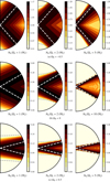Fig. 6.

Largest normalised growth rate σ/β₀ for several configurations, computed with SWAN for equatorial ellipticity β₀ = 0.2. Visualisations in a meridional section using the normalised axes x/a and z/c, with $a = \sqrt{1 + β_{0}}$ $a=\sqrt{1+\beta_0}$ , $b = \sqrt{1 - β_{0}}$ $b=\sqrt{1-\beta_0}$ , and c = 1/(ab). White dashed lines, given by formula (18), show the critical latitudes on which the growth rate is maximum as predicted by (24). For each case, the type of waves involved in parametric mechanism is specified between brackets. Dashed (grey) curves illustrate the domain of existence of ℋ₂ waves at the resonance (in the regime β₀ ≪ 1).

Therefore, the numerical analysis has confirmed and extended the asymptotic analysis. In stably stratified interiors, resonance condition (13) illustrated in Fig. 2 is a necessary and sufficient condition for tidal instability (when β₀ ≪ 1). Indeed, we have not found any other resonance yielding larger growth rates than the ones at the sub-harmonic resonance. In the orbital range −1 ≤ Ω₀ ≤ 3, tidal instability is triggered by sub-harmonic resonances of inertia-gravity waves. Moreover, there is an equatorial trapping of tidal instability between conical latitudes, depending on the orbital configuration according to formula (18). At these latitudes, the wave vector is parallel to the gravity field, such that the maximum growth rate is unaffected by the stable stratification.

3.4. Leading-order (laminar) diffusive effects

We reintroduce now the leading-order (laminar) diffusive effects at the onset of tidal instability. In the diffusive regime, tidal instability is triggered if the largest diffusionless growth rate σ overcomes the (negative) laminar damping rates due to viscosity τ_ν, radiative diffusivity τ_κ and Joule diffusion τ_Ω. Hence, the diffusionless growth rate σ ought to be reduced by the laminar damping rates, yielding the diffusive growth rate

$\begin{matrix} σ_{D} = σ + (τ_{ν} + τ_{κ} + τ_{Ω}) . \end{matrix}$ $\begin{aligned} \sigma _\mathcal{D} = \sigma + \left( \tau _\nu + \tau _\kappa + \tau _\Omega \right). \end{aligned}$ (28)

We have confirmed in Sect. 3.3 that tidal instability is a parametric instability, involving only inertial and/or gravito-inertial waves in radiative interiors. Consequently, we can simply estimate the laminar damping rates by computing the damping rates of the inertial and gravito-inertial waves involved in the triadic couplings. Indeed, triadic couplings can only give non-vanishing growth rates (28) if the waves individually exist, that is if they are not damped by any diffusive effect before being efficiently nonlinearly coupled. We have shown in Sect. 3.3 that the diffusionless growth rate σ is maximum on critical latitudes, where the wave vector satisfies k₀ × g = 0 (when β₀ ≪ 1). Then, in the local plane-wave model, the buoyancy term in the local vorticity equation (which is proportional to k₀ × g) vanishes such that vorticity and energy equations are uncoupled (in the local formalism). This means that these waves are locally insensitive to stratification on the critical latitudes, yielding τ_κ = 0. Thus, in the absence of background turbulent motions (see the discussion in Sect. 3.5), the waves are individually damped by viscosity and Joule diffusion (in the weak field regime Le ≪ 1).

For the stability computations, we rewrite here the magnetic field as

$\begin{matrix} B = B_{0} + b, \end{matrix}$ $\begin{aligned} \boldsymbol{B} = \boldsymbol{B}_0 + \boldsymbol{b}, \end{aligned}$ (29)

where the fossil field B₀ is assumed to be steady here. The pervading fossil magnetic fields are nearly axisymmetric and dipole-dominated at the leading order, as observed in magnetic binaries (e.g. Alecian et al. 2016; Landstreet et al. 2017; Kochukhov et al. 2018; Shultz et al. 2017, 2018). For the stability computations, we assume a fossil field of the form B₀ ∝ 1_z, with a dimensionless strength measured by the Lehnert number Le. The presence of other field components only slightly modifies the frequencies of inertial and inertial-gravity waves at the onset. We also expect the damping rates to have a similar behaviour in the laminar regime. In the weak field regime Le ≪ 1, the damping rates have been devised by Sreenivasan & Narasimhan (2017) in the local theory and by Kerswell (1994) in the global one. They depend on the wave properties, that is here the wave vector. Notably, we explain in Appendix C why the mixed couplings between inertial waves and slow MC waves cannot lead to tidal instability in short-period binaries (in the presence of Joule diffusion). Hence, we remind the reader that only parametric resonances of inertial and gravito-inertial waves can generate tidal instability in the presence of magnetic fields.

Then, the viscous and the Joule damping rates in the weak field regime (Le ≪ 1) in any z-plane read

$\begin{matrix} τ_{ν} & = - | k_{0} |^{2} E k, \end{matrix}$ $\begin{aligned} \tau _\nu&= - |\boldsymbol{k}_0|^2 \, Ek, \end{aligned}$ (30a)

$\begin{matrix} τ_{Ω} & = - \frac{{cos}^{2} (θ_{0}) {| k_{0} |}^{4} E m L e^{2}}{4 {cos}^{2} (θ_{0}) + {| k_{0} |}^{4} E m^{2}} | 1 - Ω_{0} |, \end{matrix}$ $\begin{aligned} \tau _\Omega&= - \frac{\cos ^2 (\theta _0) \, |\boldsymbol{k}_0|^4 Em \, Le^2}{4 \cos ^2 (\theta _0) + |\boldsymbol{k}_0|^4 \, Em^2} \, |1-\Omega _0|, \end{aligned}$ (30b)

with |k₀| the norm of the wave vector at the resonance (and at the initial time) and cos(θ₀) given by condition (18). Expression (30b) is quantitatively valid when B₀ ∝ 1_z (Sreenivasan & Narasimhan 2017). In the regime Pm ≪ 1, laminar Joule diffusion is the leading-order dissipative effect (|τ_Ω| ≫ |τ_ν|). The Joule damping has already been considered for homogeneous fluids (Kerswell 1994; Herreman et al. 2009, 2010; Cébron et al. 2012a). Note that formula (30b) is exactly the Joule damping rate of tidal instability in neutral fluids ( ${\tilde{N}}_{0} = 0$ $\widetilde{N}_0=0$ ). Besides, formulas of Herreman et al. (2009) and Cébron et al. (2012a) are recovered in the limit |k₀| ≫ 1, by using the resonance condition 2cos θ₀ = ±1 to set θ₀ for ${\tilde{N}}_{0} = 0$ $\widetilde{N}_0=0$ . Formula (30b) has two asymptotic behaviours, depending on the value of k₀. They are separated by the condition

$\begin{matrix} | k_{0} | = \sqrt{2 cos (θ_{0}) / E m} \sim E m^{- 1 / 2} . \end{matrix}$ $\begin{aligned} |\boldsymbol{k}_0| = \sqrt{2 \cos (\theta _0) /Em} \sim Em^{-1/2}. \end{aligned}$ (31)

On the one hand, we obtain a wave-dominated regime when |k₀| ≤ Em^−1/2, in which the Joule damping rate scales as τ_Ω ∝ −Em Le²|k₀|⁴/4. On the other hand, we get a diffusion-dominated regime when |k₀| ≥ Em^−1/2. In the latter regime, the damping rate is independent of the wave vector and scales as τ_Ω ∝ −Le²/Em.

We illustrate in Fig. 7 the evolution of Joule damping rate (30b) in the different regimes. Tidal instability will survive in the presence of magnetic fields if σ ≫ |τ_Ω|. Typical values of the diffusionless growth rate, given by formula (24), are σ ∼ 𝒪(β₀) with β₀ ∈ [10⁻⁴, 10⁻²] in close binaries. We clearly observe that tidal instability does survive against Joule diffusion, for short-wavelength perturbations with |k₀| ≤ 10⁴ − 10⁵. For larger values of the wave number, the Joule damping rate always overcomes the diffusionless growth rate, such that no instability is triggered.

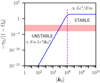Fig. 7.

Dimensionless Joule damping −τ_Ω/|1 − Ω₀| of tidal instability (solid blue line), as a function of magnitude |k₀|. Dashed magenta line is given by formula (31), delimiting the two hydromagnetic regimes. Red shaded areas show the typical strength of the diffusionless growth rate of tidal instability σ ∼ 𝒪(β₀), with β₀ ∈ [10⁻⁴, 10⁻²] for close binaries. Computations at Le = 10⁻⁵ and Ek/Pm = 10⁻¹² for the dimensionless fossil field B₀ = 1_z aligned with the spin axis.

3.5. Other dissipative mechanisms

At the linear onset, the laminar diffusive effects discussed in Sect. 3.4 are always present, but we have shown that they are smaller than the largest diffusionless growth rate σ. Hence, these effects can be reasonably neglected at the onset, yielding σ_𝒟 ∼ σ. However, other diffusive effects do exist in stellar interiors, which may weaken the growth of tidal instability.

Phase mixing is known to provide a significant source of Joule heating, by dissipating Alfvén (and magneto-sonic) waves in stellar atmospheres (e.g. Heyvaerts & Priest 1983) or stellar interiors (Spruit 1999). Yet, phase-mixing is probably irrelevant for tidal instability in the weak field regime (Le ≪ 1), notably because Aflvén waves are not involved in tidal instability (see Appendix C). Whether phase-mixing could increase the dissipation of inertial and gravito-inertial waves in stellar interiors remains unknown and is largely beyond the scope of the present study.

In the presence of an innermost convective envelope, inertial and gravito-inertial waves can exhibit singular shear layers, reminiscent of wave attractors (e.g. Dintrans et al. 1999; Rieutord & Valdettaro 2010, 2018; Mirouh et al. 2016; Lin & Ogilvie 2017). These global wave patterns are not directly involved in the parametric mechanism of tidal instability, but they fill the whole fluid domain and may provide an additional bulk damping rate for tidal instability. Indeed, these structures can be destabilised in the nonlinear regime (Jouve & Ogilvie 2014), possibly yielding small-scale instabilities. Brunet et al. (2019) showed that the resulting small-scale turbulence in the bulk could be well modelled by a turbulent eddy diffusion. In particular, anisotropic shear-driven turbulence may be generated (e.g. Zahn 1992). In such a case, Garaud et al. (2017) and Gagnier & Garaud (2018) proposed to model the local shear-driven turbulence by introducing the turbulent viscosity

$\begin{matrix} ν_{t} \propto 0.08 κ_{T} / J, J = N_{0}^{2} / S^{2}, \end{matrix}$ $\begin{aligned} \nu _\mathrm{ t} \propto 0.08 \, \kappa _{\rm T}/J, \ \, \ J = N_0^2/S^2, \end{aligned}$ (32)

with κ_T the radiative diffusivity, J the local gradient Richardson number and S the local shearing rate (responsible for the shear instabilities). The stability criterion for shear instabilities is apparently JPr ≃ 0.007 (Garaud et al. 2017). Then, prediction (32) would yield an upper-bound effective turbulent Ekman number Ek_t ≤ 10⁻¹⁰ for speculative stellar values, to use in expression (30a) for the viscous damping rate. For the range of wave numbers |k₀| given in Fig. 7, we find that the associated turbulent damping rate is smaller than the diffusionless growth rate σ (not shown). Therefore, even in the presence of shear-driven instabilities, the associated turbulent damping can be ignored at the onset of tidal instability for the (strong enough) tidal deformations considered in this work (β₀ ∼ 10⁻³ − 10⁻², see Table 2).

Table 2.

Physical and orbital characteristics of non-synchronised and non-magnetic binary systems, surveyed by the BinaMIcS Collaboration (Alecian et al., in prep.).

4. Turbulent mixing due to nonlinear tidal flows

At this stage, we have shown that tidal instability can be triggered within stably stratified interiors, even against the stabilising effect of a background (fossil) magnetic field in the weak field regime (Le ≪ 1). The next step is to characterise the saturated regime of tidal flows. Modelling turbulent mixing in radiative interiors is one of the enduring problems in stellar dynamics (e.g. Zahn 1974). Several studies have examined the turbulence in radiative zones (e.g. Zahn 1992; Mathis et al. 2004, 2018; Garaud et al. 2017; Gagnier & Garaud 2018). Yet, these models focus on shear-driven turbulence. Hence, tidally driven turbulence in binaries remains to be described. Numerical simulations have shown that small-scale turbulence can be excited by tidal instability (Barker & Lithwick 2013a,b; Le Reun et al. 2017), possibly leading to global tidal mixing (Vidal et al. 2018). Thus, tidal mixing is expected in radiative interiors. We motivate our assumptions in Sect. 4.1. Then, we use dimensional-type arguments in Sect. 4.2 to develop a phenomenological description of the nonlinear tidal mixing in radiative interiors in Sect. 4.3, valid in the orbital range −1 ≤ Ω₀ ≤ 3. Finally, we assess its validity by using proof-of-concept simulations in Sect. 4.4.

4.1. Assumptions

As shown in Sect. 3, magnetic effects play a minor role at the onset of instability in the orbital range −1 ≤ Ω₀ ≤ 3. They essentially weaken the growth rate of tidal instability, due to the laminar Joule damping. In the (transient) linear growth, the fossil field B₀ is not much affected by tidal flows, which are not expected to generate significant mixing. It only decays on the slow (laminar) Joule diffusion time, which is much larger than the timescale for the onset of tidal instability for stellar parameters. This phenomenon is well-known in global models of resistive magnetohydrodynamics, also known as free-decay of magnetic fields (e.g. Moffatt 1978). However, in the saturated regime, the fossil field would interact nonlinearly with the nonlinear tidal flows, as governed by induction equation

$\begin{matrix} \frac{\partial B}{\partial t} = \nabla \times [(U_{0} + u) \times B] + \frac{Ek}{Pm} \nabla^{2} B, \end{matrix}$ $\begin{aligned}&\frac{\partial \boldsymbol{B}}{\partial t} = \boldsymbol{\nabla } \times \left[ (\boldsymbol{U}_0 + \boldsymbol{u}) \times \boldsymbol{B} \right] + \frac{Ek}{Pm} \, \boldsymbol{\nabla }^2 \boldsymbol{B}, \end{aligned}$ (33a)

$\begin{matrix} \nabla \cdot B = 0, B (r, t = 0) = B_{0} (r), \end{matrix}$ $\begin{aligned}&\boldsymbol{\nabla } \boldsymbol{\cdot } \boldsymbol{B} = 0, \ \, \ \boldsymbol{B} (\boldsymbol{r},t=0) = \boldsymbol{B}_0 (\boldsymbol{r}), \end{aligned}$ (33b)

in which the initial time t = 0 refers now to an initial time just after the growth of the instability. In Eq. (33a), the nonlinear velocity field u is governed by momentum Eq. (3a). In the relevant weak field regime Le ≪ 1, nonlinear numerical simulations of the coupled problems showed that magnetic effects do not weaken the turbulent tidal flows (Barker & Lithwick 2013b; Cébron & Hollerbach 2014; Vidal et al. 2018). These turbulent flows generate mixing, that would ultimately increase the Ohmic diffusion of the fossil field B₀. Therefore, Ohmic diffusion ought to be increased (a priori). This is often modelled by introducing a turbulent magnetic diffusivity (e.g. Kitchatinov et al. 1994; Yousef et al. 2003; Käpylä et al. 2019). In this configuration, the initial fossil field is expected to decay on somehow faster timescales, due to the presence of mixing generated by tidal instability. This situation strongly differs from the picture of ideal magnetohydrodynamics, in which the laminar decay of the fossil field is small (and so can be sometimes neglected). Note that an initial fossil field may still be in quasi-equilibrium with tidal flows, if the dissipated field is continuously regenerated by some kind of dynamo action. However, dynamo action of tidal flows in strongly stratified interiors remains elusive (Vidal et al. 2018) and will not be investigated here. Consequently, to estimate the fossil field decay due to tidal instability, we must estimate the turbulent magnetic diffusivity generated by the saturation of tidal instability.

4.2. Mixing-length theory

Estimating a realistic turbulent magnetic diffusivity is challenging, because no numerical model cannot probe accurately the stellar conditions. This makes the relevance of numerical results sometimes elusive. Therefore, we aim to build asymptotic scaling laws for the tidal mixing, based on dimensional-type arguments that embrace both numerical and stellar conditions. To estimate the local tidal mixing in stratified interiors, we develop a mixing-length theory, by analogy with mixing-length arguments commonly used for shear-driven turbulence in radiative interiors of stars (e.g. Zahn 1992; Mathis et al. 2004, 2018).

In turbulent flows, the laminar viscosity is often replaced by an effective eddy (turbulent) viscosity, usually modelled by using mixing-length theory in stellar contexts. In hydromagnetic turbulence, Yousef et al. (2003) and Käpylä et al. (2019) argued that in the weak field regime (Le ≪ 1) the turbulent magnetic Prandtl number is not far from unity. Hence, the turbulent magnetic diffusivity can be a priori modelled by mixing-length type predictions. This is supported by local hydromagnetic simulations of the three-dimensional turbulence generated by tidal instability (Barker & Lithwick 2013b). They showed that weak magnetic fields can even favour the small-scale tidal turbulence. Global tidal mixing has also been found in global stratified models (Vidal et al. 2018). Thus, we may replace any laminar diffusivity (denoted 𝒟) by an effective eddy diffusivity (denoted 𝒟_t), induced by the nonlinear tidal flows. Then, mixing-length theory (e.g. Tennekes & Lumley 1972) predicts in dimensional form (up to a unknown proportional constant)

$\begin{matrix} D_{t} \propto \frac{1}{3} u_{t} l_{t}, \end{matrix}$ $\begin{aligned} \mathcal{D} _\mathrm{ t} \propto \frac{1}{3} u_\mathrm{ t} \, l_\mathrm{ t}, \end{aligned}$ (34)

where u_t and l_t are respectively the typical (dimensional) local velocity and length scale of the turbulent motions. Note that u_t is the typical amplitude of the nonlinear tidal flows. This must not be confused with the amplitude u_w of the waves that are excited by the forcing mechanism (see the case of internal gravity waves in Rogers & McElwaine 2017). Here, u_w is much smaller than u_t in amplitude. Hence, the eddy diffusivity 𝒟_t is a local property of the nonlinear flows, rather than a property of the fluid (or of the wave amplitude). The key point to apply formula (34) is to find accurate predictions for u_t and l_t in the nonlinear regime of tidal instability.

On the one hand, we have shown in Sect. 3 that tidal instability is generated by sub-harmonic resonances of inertial waves, more or less modified by the gravity field in the orbital range −1 ≤ Ω₀ ≤ 3. This mechanism holds whatever the strength of stratification, measured by the ratio N₀/Ω_s. Therefore, the turbulent velocity scale u_t should not depend (strongly) on the local strength of stratification N₀/Ω_s. This is supported by proof-of-concept simulations (see Fig. 2b in Vidal et al. 2018), showing that nonlinear tidal flows exhibit the scaling devised in homogeneous fluids (Barker & Lithwick 2013a; Grannan et al. 2016). This reads

$\begin{matrix} u_{t} \sim α_{1} β_{0} r_{l} Ω_{s} (1 - Ω_{0}) \end{matrix}$ $\begin{aligned} u_\mathrm{ t} \sim \alpha _1 \beta _0 r_{\rm l} \, \Omega _\mathrm{ s} (1 - \Omega _0) \end{aligned}$ (35)

with r_l ≤ R the local position and α₁ ∼ 0.3–0.5 a dimensionless pre-factor obtained numerically both in homogeneous (Grannan et al. 2016, estimated from Fig. 4d) and strongly stratified tidal flows (Vidal et al. 2018, estimated from Fig. 2b). Hence, we reasonably estimate the turbulent velocity u_t by using prescription (35). On the other hand, l_t should depend on the local ratio N₀/Ω_s. Several regimes have been found in forced stratified turbulence (e.g. Brethouwer et al. 2007).

4.3. Phenomenological prescriptions

4.3.1. Weakly stratified regime (N₀/Ω_s ≤ 1)

In the weakly stratified regime, characterised by N₀/Ω_s ≤ 1, ℋ₁ waves satisfying the sub-harmonic resonance condition are barely affected by stratification. We estimate l_t by balancing the nonlinear term (u⋅∇) u with the injection term (u⋅∇) U₀ in momentum Eq. (3a). This yields the typical turbulent length scale in dimensional form l_t ∝ α₁r_l. Then, the weakly stratified regime is characterised by the eddy diffusivity (in dimensional form)

$\begin{matrix} D_{t} \propto \frac{1}{3} α_{1}^{2} β_{0} r_{l}^{2} Ω_{s} (1 - Ω_{0}) . \end{matrix}$ $\begin{aligned} \mathcal{D} _\mathrm{ t} \propto \frac{1}{3} \alpha _1^2 \beta _0 r_\mathrm{ l}^2 \, \Omega _\mathrm{ s} (1 - \Omega _0). \end{aligned}$ (36)

Formula (36) predicts a roughly homogeneous mixing in the weakly stratified regime, as found in global models (Grannan et al. 2016; Vidal et al. 2018) in which r_l ≃ R. This explains why the tidal mixing computed in Vidal et al. (2018) is roughly constant as a function of stratification, when N₀/Ω_s ≤ 1 (see their Fig. 9). However, estimate (36) may be reduced in this regime due to (compressible) density variations (close to the isentropic profile when N₀/Ω_s ≪ 1).

Finally, formula (36) provides a good estimate of the leading-order term in the eddy diffusivity tensor (e.g. Dubrulle & Frisch 1991; Wirth et al. 1995). In addition, note that rotation would also support small anisotropic diffusion in the axial direction (Tilgner 2004; Elstner & Rüdiger 2007).

4.3.2. Stratified regimes (N₀/Ω_s ≥ 1)

We now investigate the stratified regimes N₀/Ω_s ≥ 1. Stratified turbulence is highly anisotropic. Indeed, a commonly observed feature of strongly stratified flows is the formation of quasi-horizontal layers, often described as pancake structures (e.g. Billant & Chomaz 2001). Such layers are conspicuous in simulations of tidal flows in strongly stratified fluids, both in non-rotating (Le Reun et al. 2018) and rotating fluids (Vidal et al. 2018). Hence, l_t depends on both the direction and the strength of stratification. We introduce two turbulent length scales, respectively $l_{t}^{∥}$ $l_\mathrm{t}^\parallel$ in the normal direction (that is along the gravity field) and $l_{t}^{⊥}$ $l_\mathrm{t}^\perp$ in the other horizontal directions.

Several regimes of stratified turbulence have been devised in fundamental fluid mechanics (Billant & Chomaz 2001; Brethouwer et al. 2007). They are characterised by the buoyancy Reynolds number

$\begin{matrix} R \sim \frac{u_{t}^{3}}{l_{t}^{⊥} N_{0}^{2} ν} \cdot \end{matrix}$ $\begin{aligned} \mathcal{R} \sim \frac{u_\mathrm{ t}^3}{l_\mathrm{ t}^\perp N_0^2 \nu }\cdot \end{aligned}$ (37)

Le Reun et al. (2018) investigated the small-scale turbulence sustained by tides in the regime ℛ ≤ 1, in which vertical viscous shearing is significant. However, radiative interiors are in the opposite regime ℛ ≫ 1 (Mathis et al. 2018). Moreover, they neglected rotation, by setting Ω_s = 0. In such a configuration, the subspaces of waves [ℋ₁, ℋ₂] at the sub-harmonic resonance are empty, according to dispersion relations (15). Hence, tidal instability can only involve sub-harmonic resonances of internal waves ℋ₂ in the limit N₀/Ω_s → ∞ and |Ω₀|→∞. Therefore, their results do not apply for our astrophysical problem, for any orbit in the range −1 ≤ Ω₀ ≤ 3. In the relevant strongly stratified regime (ℛ ≫ 1), diffusion is unimportant and the turbulence is three-dimensional (Brethouwer et al. 2007). The general scalings of this regime have been confirmed by turbulence simulations (e.g. Godeferd & Staquet 2003; Maffioli & Davidson 2016). Thus, they can be applied to the tidal problem. In addition, rotational effects are also significant within the orbital range −1 ≤ Ω₀ ≤ 3, even for large values of N₀/Ω_s ≥ 10. Hence, the resulting turbulence undergoes the combined action of stratification and rotation.

In rotating stratified turbulence, the two turbulent length scales are related by (Billant & Chomaz 2001)

$\begin{matrix} l_{t}^{⊥} \sim α_{2} \frac{N_{0}}{Ω_{s}} l_{t}^{‖} . \end{matrix}$ $\begin{aligned} l_\mathrm{ t}^\perp \sim \alpha _2 \frac{N_0}{\Omega _\mathrm{ s}} l_\mathrm{ t}^\parallel . \end{aligned}$ (38)

with α₂ ∼ 0.6 a (numerical) pre-factor constrainted from local turbulent simulations in rapidly rotating and strongly stratified turbulent regime (Reinaud et al. 2003; Waite & Bartello 2006). This regime is expected to be valid for radiative interiors, notably to describe shear-driven turbulence (Mathis et al. 2018). For strong stratification (N₀/Ω_s ≥ 10), we combine the two balances obtained by equating (i) the nonlinear term with the buoyancy force in momentum Eq. (3a) and (ii) the injection term (u⋅∇) T₀ and the nonlinear term (u⋅∇) Θ in energy Eq. (3b). These balances yield respectively

$\begin{matrix} \frac{u_{t}^{2}}{l_{t}^{‖}} \sim α_{T} g_{0} Θ_{t} and α_{T} g_{0} Θ_{t} \sim N_{0}^{2} l_{t}^{‖}, \end{matrix}$ $\begin{aligned} \frac{u_\mathrm{ t}^2}{l_\mathrm{ t}^\parallel } \sim \alpha _{\rm T} { g}_0 \, \Theta _\mathrm{ t} \ \, \ \mathrm{ and} \ \, \ \alpha _{\rm T} { g}_0 \, \Theta _\mathrm{ t} \sim N_0^2 \, l_\mathrm{ t}^\parallel , \end{aligned}$ (39)

where Θ_t is the typical dimensional turbulent buoyancy perturbation. We recover from balances (39) the classical scaling for the turbulent length scale in the normal direction, that is $u_{t} ~ l_{t}^{∥} N_{0}$ $u_\mathrm{t} \sim l_\mathrm{t}^\parallel N_0$ (e.g. Billant & Chomaz 2001; Brethouwer et al. 2007). Hence, the turbulent length scale along the gravity direction is

$\begin{matrix} l_{t}^{‖} \sim α_{1} β_{0} r_{l} (1 - Ω_{0}) \frac{Ω_{s}}{N_{0}} (with α_{1} \sim 0.3 - 0.5) . \end{matrix}$ $\begin{aligned} l_\mathrm{ t}^\parallel \sim \alpha _1 \beta _0 \, r_\mathrm{ l} \, (1-\Omega _0) \frac{\Omega _\mathrm{ s}}{N_0} \ \, \ (\mathrm{ with} \ \,\ \alpha _1 \sim 0.3 {-} 0.5). \end{aligned}$ (40)

Scaling (40) shows that tidal mixing falls in the asymptotic regime of strongly stratified turbulence (Brethouwer et al. 2007). Then, we obtain two prescriptions for the eddy diffusivity, the first one $D_{t}^{∥}$ $\mathcal{D}_\mathrm{t}^\parallel$ valid in the gravity direction and the second one 𝒟_t in the perpendicular (horizontal) directions. They yield

$\begin{matrix} D_{t}^{‖} & \propto \frac{1}{3} α_{1}^{2} β_{0}^{2} r_{l}^{2} Ω_{s} {(1 - Ω_{0})}^{2} \frac{Ω_{s}}{N_{0}}, \end{matrix}$ $\begin{aligned} \mathcal{D} _\mathrm{ t}^\parallel&\propto \frac{1}{3} \alpha _1^2 \, \beta _0^2 \, r_\mathrm{ l}^2 \, \Omega _\mathrm{ s} (1 - \Omega _0)^2 \frac{\Omega _\mathrm{ s}}{N_0}, \end{aligned}$ (41a)

$\begin{matrix} D_{t}^{⊥} & \propto \frac{1}{3} α_{1}^{2} α_{2} β_{0}^{2} r_{l}^{2} Ω_{s} {(1 - Ω_{0})}^{2}, \end{matrix}$ $\begin{aligned} \mathcal{D} _\mathrm{ t}^\perp&\propto \frac{1}{3} \alpha _1^2 \alpha _2 \, \beta _0^2 \, r_\mathrm{ l}^2 \, \Omega _\mathrm{ s} (1 - \Omega _0)^2, \end{aligned}$ (41b)

with α₁ ∼ 0.3–0.5 and α₂ ∼ 0.6 (see above). Prescriptions (41) show that the eddy diffusivity should have a quadratic dependence with the equatorial ellipticity, in any spatial direction. Another interesting prediction in this regime is that the turbulent potential and kinetic energies, defined by (in dimensional variables)

$\begin{matrix} E_{t} (Θ^{*}) \sim \frac{1}{2} \frac{α_{T}^{2} g_{0}^{2}}{N_{0}^{2}} Θ_{t}, E_{t} (u^{*}) \sim \frac{1}{2} u_{t}^{2}, \end{matrix}$ $\begin{aligned} E_\mathrm{ t}(\Theta ^*) \sim \frac{1}{2} \frac{\alpha ^2_{\rm T} { g}_0^2}{N_0^2} \Theta _\mathrm{ t}, \ \, \ E_\mathrm{ t}(\boldsymbol{u}^*) \sim \frac{1}{2} u_\mathrm{ t}^2, \end{aligned}$ (42)

are comparable in magnitude (Billant & Chomaz 2001). This can be checked in the numerical simulations (see below).

In-between the two aforementioned stratified regimes, when 1 ≤ N₀/Ω_s ≤ 10, the situation is unclear. Indeed, Vidal et al. (2018) found that u⋅g, which is responsible for tidal mixing in the normal direction, is largely unaffected by stratification when N₀/Ω_s ≤ 10 (see their Fig. 4). Hence, we may extend prescription (36) for the turbulent mixing up to N₀/Ω_s ≤ 10. Yet, this behaviour is not conspicuous in the numerics (see Fig. 9b in Vidal et al. 2018). This may be due to the rather specific numerical method, which inaccurately probed the intermediate regime 1 ≤ N₀/Ω_s ≪ 10. Thus, a transition may be also expected between the two regimes (36) and (41) when 1 ≤ N₀/Ω_s ≤ 10.

4.4. Validation against numerical simulations

We assess the relevance of predictions (36) and (41) by using direct numerical simulations. To do so, we solve nonlinear and diffusive Eqs. (3) in a global model. We supplement the governing equations by considering the stress-free conditions

$\begin{matrix} u \cdot 1_{n} = 0, 1_{n} \times [(\nabla u + {(\nabla u)}^{⊤}) 1_{n}] = 0, \end{matrix}$ $\begin{aligned} \boldsymbol{u} \boldsymbol{\cdot } \boldsymbol{1}_n = 0, \ \, \ \boldsymbol{1}_n \times \left[ (\boldsymbol{\nabla } \boldsymbol{u} + (\boldsymbol{\nabla } \boldsymbol{u})^\top ) \, \boldsymbol{1}_n \right] = \boldsymbol{0}, \end{aligned}$ (43)

and assuming a fixed temperature Θ = 0 at the boundary. Stress-free conditions (43) are known to lead to spurious numerical behaviours, associated with the evolution of angular momentum in weakly deformed spheres (Guermond et al. 2013). To circumvent this numerical problem, we follow Cébron & Hollerbach (2014) and Vidal et al. (2018) by imposing a zero-angular momentum for the velocity perturbation. Moreover, the external region is assumed to be electrically insulating, such that the magnetic field b matches a potential field at the boundary.

For the computations, we use the proof-of-concept global numerical model introduced in Vidal et al. (2018). Briefly, the reference ellipsoidal configuration (described in Sect. 2.3) is approximated in spherical geometry by an spatially varying equatorial ellipticity profile ϵ(r, β₀), depending of the ellipticity β₀ of the ellipsoidal configuration. This profile is chosen such that the reference configuration satisfies all the aforementioned boundary conditions in the spherical geometry. The simulations have been performed with the open-source nonlinear code XSHELLS¹, described in Schaeffer et al. (2017) and validated against standard spherical benchmarks (Marti et al. 2014; Matsui et al. 2016). A second-order finite difference scheme is used in the radial direction. The angular directions are discretised using a pseudo-spectral spherical harmonic expansion, provided by the SHTns library (Schaeffer 2013). The time-stepping scheme is of second order in time and treats the diffusive terms implicitly, while the nonlinear and Coriolis terms are handled explicitly. We refer the reader to Vidal et al. (2018) for additional methodological details of the tidal problem.

To estimate the turbulent magnetic diffusivity in a global model, we measure the decay of an initial large-scale magnetic field (Yousef et al. 2003; Käpylä et al. 2019) in the presence of nonlinear tides, to compare it with the free decay rate of the same magnetic configuration in laminar diffusive models (e.g. Moffatt 1978). We compute the (dimensionless) decay rate σ_η ≤ 0 of the volume average of the magnetic energy over the computational integration time T as

$\begin{matrix} σ_{η} = lim_{T \to \infty} \frac{1}{T} log (\int_{V} \frac{1}{2} {| B |}^{2} d V) . \end{matrix}$ $\begin{aligned} \sigma _\eta = \lim \limits _{T\rightarrow \infty } \frac{1}{T} \log \left( \int _{\mathcal{V} } \frac{1}{2} |\boldsymbol{B}|^2 \, \mathrm{d} \mathcal{V} \right). \end{aligned}$ (44)

Decay rate (44) is a global estimate in the simulations of the effective diffusivity 𝒟_t. Käpylä et al. (2019) measured in a similar way the turbulent diffusivity, obtaining a good quantitative agreement with mean-field analyses. Then, global decay rate (44) should have the same scaling law in β₀ for all the initial magnetic fields B₀, even if the (numerical) pre-factors will be different. Indeed, all the magnetic components will not obey the same scaling law in the strongly stratified regime (due to the anisotropic mixing). Notably, we expect toroidal magnetic fields, satisfying B₀⋅1_n = 0 (at any position), to be preferentially dissipated in the normal direction. Thus, scaling (41a) should apply predominantly for toroidal fields. On the contrary, we expect the dissipation of poloidal magnetic fields (with predominant components in the normal direction) to obey scaling (41b) in the horizontal directions. However, we emphasise that the pre-factors obtained from numerical simulations, performed for conditions far-removed from the astrophysical regimes, are often irrelevant for astrophysical problems (compared to mixing-length predictions). We only focus on the dependence in β₀, which should be generic whatever the topology of the initial magnetic field in the numerics. Thus, we aim at recovering (i) σ_η ∝ β₀ for weakly stratified regime (36) and (ii) $σ_{η} \propto β_{0}^{2}$ $\sigma_\eta \propto \beta_0^2$ for strongly stratified regime (41).

In magnetic radiative stars, the initial fossil field is unlikely force-free (e.g. Duez & Mathis 2010; Duez et al. 2010), except possibly close to the stellar surface. The exact topology of the field does depend on the Lorentz force, and only magnetic equilibria involving poloidal and toroidal components have been found (e.g. Braithwaite & Spruit 2017). Then, in addition to the slow laminar Joule diffusion, Braithwaite & Cantiello (2012) showed that an initial fossil field can decay due to the propagation of (slow) Magneto-Coriolis waves (see Appendix B) in the presence of rotation. Such a magnetic decay occurs on the (rather slow) dynamical timescale

$\begin{matrix} τ_{MC} \sim {(Ω_{s} L e^{2})}^{- 1} . \end{matrix}$ $\begin{aligned} \tau _\mathrm{ MC} \sim (\Omega _{\rm s} Le^2)^{-1}. \end{aligned}$ (45)

Moreover, the field can be also dissipated by the turbulent mixing generated by nonlinear tidal flows. Thus, the initial field can be dissipated simultaneously by several mechanisms if we neglect in-situ dynamo mechanisms, that would regenerate the field against laminar and turbulent diffusion but are highly debated.

However, we would like the magnetic decay to be insensitive to dynamical evolution (45) in the numerics, to investigate only the turbulent effects in a well controlled set-up. Hence, we aim to find a magnetic configuration in which the initial field would decay solely by laminar Joule diffusion in the absence of tides. To do so, we can reasonably switch-off the Lorentz force in momentum equation, to estimate turbulent magnetic diffusivity (44) for a given initial magnetic field. Without magnetic forces, MC waves are no longer sustained in the system. Moreover, as explained above, the Lorentz force surprisingly plays a negligible role² on the turbulent mixing generated by nonlinear tidal flows in the (relevant) weak field regime Le ≪ 1 (Barker & Lithwick 2013b; Cébron & Hollerbach 2014; Vidal et al. 2018). Consequently, for this particular problem of tidal instability, neglecting the Lorentz force is advisable in the numerics.

As a reference configuration, we have assumed Ω₀ = 0. Indeed, we have shown theoretically in Sect. 3 that the underlying mechanism of tidal instability does not change in the range −1 ≤ Ω₀ ≤ 3, and similarly the turbulent scalings (e.g. Grannan et al. 2016; Vidal et al. 2018). Hence, investigating only one orbital configuration is necessary. Then, problem (33a) reduces here to a kinematic (linear) initial value problem for the initial field. We emphasise that the exact topology of the initial field will not be essential here for the numerical model. Indeed, without the Lorentz force, induction Eq. (33a) is uncoupled to the momentum equation. To mimic the slow magnetic decay on the laminar Joule diffusion (in the absence of tides), we have chosen for the initial fossil field the least-damped, poloidal free decay magnetic mode of the sphere (see Moffatt 1978, p. 36–40). This particular magnetic field is an exact solution of the purely diffusive induction equation. It has the smallest laminar Ohmic free decay rate σ_Ω (in dimensionless form), given by

$\begin{matrix} σ_{Ω} = π^{2} Ek / Pm . \end{matrix}$ $\begin{aligned} \sigma _\Omega = \pi ^2 {Ek}/{Pm}. \end{aligned}$ (46)

Thus, this is the most suited initial magnetic field to assess the validity of the turbulent scaling laws. Indeed, slow laminar Joule diffusion (46) should not be coupled with the expected faster turbulent diffusion in the numerics to get robust results. In practice, we conducted the simulations at the fixed dimensionless numbers Ek = 10⁻⁴, Pr = 1, and Pm = 0.1. The latter value ensures that no dynamo magnetic field can grow exponentially. Our spatial discretisation is N_r = 224 radial points, l_max = 128 spherical harmonic degrees and m_max = 100 azimuthal wave numbers. We have integrated the equations on one (dimensionless) Ohmic diffusive time (Ek/Pm)⁻¹, to determine accurately the turbulent decay rate σ_η.

Figure 8 shows the representative results for the two stratified regimes. We observe that the decay rate σ_η is always larger than the free decay rate σ_Ω of the initial fossil field. Then, the striking feature is that we recover the two scalings as a function of the ellipticity, as predicted by our mixing-length theory. In the weakly stratified regime (top panel), numerical decay (44) agrees well with the linear scaling σ_η ∝ β₀, consistent with mixing-length formula (36). The agreement is even much better in the strongly stratified regime (bottom panel), obtaining the quadratic scaling $σ_{η} \propto β_{0}^{2}$ $\sigma_\eta \propto \beta_0^2$ expected from (41).

We note that the observed enhancement generated by tidal instability is rather weak in the simulations. This is not due to the tidal amplitude, which is already two orders of magnitude larger than the typical values for binaries (β₀ ≃ 10⁻¹ in the numerics and β₀ ≃ 10⁻³ − 10⁻², see Table 2 below). This simply comes from the over-estimated value of the laminar Joule diffusion in the simulations (that is Ek/Pm = 10⁻³). This makes the laminar and turbulent decay rates roughly comparable in amplitude. Simulations in the astrophysical regime (that is Ek/Pm ≤ 10⁻¹⁰) would show a stronger tidal effect. Yet, our simulations already support the trend predicted by mixing-length theory (41). For stellar conditions, the latter predicts that the tidal decay rate would be much stronger than the laminar Joule decay rate (see the discussion in Sect. 5).

Finally, the typical ratio of the volume averaged thermal and kinetic (dimensionless) energies, for the simulations in the strongly stratified regime (bottom panel of Fig. 8), is E(Θ)/E(u)=8.1 ± 3.5. This numerical value agrees very well with the theoretical scaling (42) in the strongly stratified regime (Billant & Chomaz 2001), yielding E(Θ)/E(u)∼N₀/Ω_s = 10 in dimensionless variables. This is another evidence of the validity of the mixing-length theory.

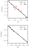Fig. 8.

Turbulent diffusion of magnetic field by tidal instability, as a function of equatorial ellipticity β₀. Ratio σ_η/|σ_Ω|, with σ_η the global decay rate (44) and σ_Ω the free decay rate (46) without tides. Simulations at Ω₀ = 0, Ek = 10⁻⁴, Pr = 1 and Pm = 0.1. Solid lines are the least-squares fits. Top panel: weakly stratified regime (N₀/Ω_s = 0), with σ_η/|σ_Ω|= − 3.09 β₀ − 1.00. Bottom panel: strongly stratified regime (N₀/Ω_s = 10) with $σ_{η} / | σ_{Ω} | = - 3.13 β_{0}^{2} - 1.21$ $\sigma_\eta/|\sigma_\Omega| = -3.13 \, \beta_0^2 -1.21$ .

5. Astrophysical discussion

We have obtained a consistent picture of tidal instability in an idealised set-up of radiative interiors. This predicts the linear onset (Sect. 3) and the nonlinear mixing induced by the saturated flows (Sect. 4). For the sake of theoretical and numerical validations, we have only considered rather idealised stellar models, described in Sect. 2. Then, the predictions have been successfully compared with proof-of-concept numerical simulations, paving the way for astrophysical applications.

Indeed, we emphasise that the theory can a priori embrace more realistic stellar conditions. In particular, the mixing-length theory is only based on local dimensional arguments, that should remain valid for more realistic conditions. Therefore, we discuss now our findings in the context of tidally deformed and stably stratified (radiative) interiors. Notably, we are in the position to build a new physical scenario, that may explain the lower incidence of fossil fields in some short-period and non-synchronised binaries (Alecian et al., in prep.).

5.1. A new scenario?

We consider a close binary system with a radiative primary of mass M₁ and a secondary of mass M₂. The primary is pervaded by an initial fossil field B₀. Note that distinction between the primary and secondary is only made for convenience, such that the situation can be reversed in the scenario (if we are interested in the secondary). The orbital and spin angular velocities are respectively Ω_orb and Ω_s. We focus on non-synchronised binaries in the orbital range −1 ≤ Ω₀ ≤ 3, where Ω₀ = Ω_orb/Ω_s is the dimensionless orbital frequency. The orbits are almost circularised, but small orbital eccentricities e ≪ 1 do not strongly modify the fate of tidal flows (Vidal & Cébron 2017). We also focus on binaries with short-period systems, with typical periods of T_s = 2π/Ω_s ≤ 10 days. Due to the combined action of the tides and the spin, the star is deformed into an triaxial ellipsoid (Chandrasekhar 1969; Lai et al. 1993; Barker et al. 2016). The latter is characterised by a typical equatorial ellipticity β₀, estimated from the static bulge theory (Cébron et al. 2012a; Vidal et al. 2018). For the bulge generated onto the primary, this reads

$\begin{matrix} β_{0} \sim \frac{3}{2} \frac{M_{2}}{M_{1}} {(\frac{R}{D})}^{3}, \end{matrix}$ $\begin{aligned} \beta _0 \sim \frac{3}{2} \frac{M_2}{M_1} \left( \frac{R}{D} \right)^3, \end{aligned}$ (47)

where R is the typical radius of the primary and D is the typical distance separating the two bodies. The density stratification of the radiative envelope is measured by the typical dimensionless ratio N₀/Ω_s, where N₀ is the typical Brunt–Väisälä frequency. A representative value for intermediate-mass stars is N₀ ∼ 10⁻³ s⁻¹ (e.g. Rieutord 2006), yielding a typical ratio N₀/Ω_s ≫ 10.

The tidal forcing sustains an equilibrium tidal velocity field (Remus et al. 2012; Vidal & Cébron 2017) in the primary fluid body. This equilibrium tidal flow can be nonlinearly coupled with inertial-gravity waves, triggering tidal instability. The dimensional growth rate σ^* of tidal instability, which does not depend on stratification, is given by

$\begin{matrix} σ^{*} = \frac{{(2 {\tilde{Ω}}_{0} + 3)}^{2}}{16 {(1 + {\tilde{Ω}}_{0})}^{2}} | Ω_{s} - Ω_{orb} | β_{0}, \end{matrix}$ $\begin{aligned} \sigma ^* = \frac{(2 \widetilde{\Omega }_0+3)^2}{16(1+\widetilde{\Omega }_0)^2} |\Omega _\mathrm{ s}-\Omega _\mathrm{ orb}| \, \beta _0, \end{aligned}$ (48)

with ${\tilde{Ω}}_{0} = Ω_{0} / (1 - Ω_{0})$ $\widetilde{\Omega}_0 = \Omega_0/(1-\Omega_0)$ . In the saturated regime, tidal instability increases the internal mixing (due to turbulence). In strongly stratified radiative interiors (N₀/Ω_s ≫ 10), the turbulent mixing generated by tidal instability is anisotropic, characterised by an eddy turbulent diffusivity $D_{t}^{∥}$ $\mathcal{D}_\mathrm{t}^\parallel$ in the direction of the self-gravity and by $D_{t}^{⊥} (≫ D_{t}^{∥})$ $\mathcal{D}_\mathrm{t}^\perp \, (\gg \mathcal{D}_\mathrm{t}^\parallel)$ in the other (horizontal) directions.

Then, the turbulent mixing will dynamically increase the Joule decay of the fossil field B₀. However, the latter field, containing both poloidal and toroidal components (to be in quasi-static magnetic equilibrium in the initial stage), will undergo an enhanced anisotropic turbulent Joule diffusion. The mechanism is illustrated in Fig. 9. On the one hand, the poloidal components, which are mainly along the normal direction, would be preferentially dissipated by the (large) eddy diffusivity $D_{t}^{⊥}$ $\mathcal{D}_\mathrm{t}^\perp$ in the horizontal directions. On the other hand, the toroidal components, trapped in the stellar interior because they have only horizontal components, are preferentially mixed by the (small) eddy diffusivity $D_{t}^{∥}$ $\mathcal{D}_\mathrm{t}^\parallel$ in the normal direction. Thus, poloidal and toroidal field lines are dissipated on different turbulent timescales. For the poloidal components which can be observed at the stellar surface, tidal instability would yield a global magnetic dissipation within the stellar interior on a few turbulent timescales τ_t (at the position r_l ≤ R), given by

$\begin{matrix} τ_{t} \propto \frac{r_{l}^{2}}{D_{t}^{⊥}} \sim \frac{K_{α}}{β_{0}^{2} Ω_{s} {(1 - Ω_{0})}^{2}} \end{matrix}$ $\begin{aligned} \tau _\mathrm{ t} \propto \frac{r_\mathrm{ l}^2}{\mathcal{D} _\mathrm{ t}^\perp } \sim \frac{K_\alpha }{\beta _0^2 \, \Omega _\mathrm{ s} (1 - \Omega _0)^2} \end{aligned}$ (49)

with the pre-factor K_α ∼ 30–50 estimated by the numerical pre-factors in formulas (41). Timescale (49) is the (fast) turbulent timescale in the perpendicular (horizontal) directions. In addition, the magnetic field would also die out in the presence of rotation on dynamical timescale (45) of the (slow) Magneto-Coriolis waves, as shown by Braithwaite & Cantiello (2012).

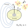Fig. 9.

Anisotropic turbulent diffusion, generated by tidal instability, of poloidal (dotted) and toroidal (dashed) field lines of fossil field B₀. A possible innermost convective core is represented.

5.2. Non-magnetic binaries

We assess here the relevance of the tidal scenario for short-period massive binary systems. Non-magnetic and non-synchronised (Ω₀ ≠ 1) binaries are given in Table 2. They have been surveyed by the BinaMIcS Collaboration (Alecian et al., in prep.). The predictions of the tidal scenario for these binary systems are given in Table 3. All these close-binaries are rapidly rotating and undergo strong tidal effects (in the two bodies), as measured by the large values of the ellipticity β₀ ∼ 10⁻³ − 10⁻². The strong tides should trigger quickly tidal instability, growing on the typical timescale (σ^*)⁻¹ ≃ 𝒪(10³) years. This is much shorter than the lifetime of these stars, about τ_MS ∼ 10⁹ years for a star of mass M₁ = 2 M_⊙ on the main sequence. Hence, tidal instability is likely to be present in these non-synchronised binaries.

Table 3.

Predictions of tidal scenario for (non-magnetic) close binaries described in Table 2.

Then, typical values for turbulent timescale (49) are τ_t ∈ [10³, 10⁷] years, except for HD 23642 and HD 32964 which are less affected by tidal instability (smaller β₀). Thus, the turbulent Joule diffusion of the initial fossil fields may occur on timescales much shorter than the stellar lifetime, typically τ_t/τ_MS ≪ 10⁻³ for the most favourable systems. Turbulent timescale (49) is also often smaller that the timescale for the laminar Ohmic diffusion of the magnetic field in the absence of turbulence τ_Ω ∝ (Ω_s Ek/Pm)⁻¹. As illustrated in Fig. 10, we get τ_t/τ_Ω ≤ 10⁻² (except for HD 23642 and HD 32964). Similarly, for several systems, τ_t is smaller than the dynamical timescale τ_MC proposed by Braithwaite & Cantiello (2012), given by expression (45).

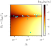Fig. 10.

Turbulent magnetic decay τ_t (49) of fossil fields, normalised by laminar Ohmic timescale τ_Ω ∼ (Ω_s Ek/Pm)⁻¹, as a function of equatorial ellipticity β₀ and dimensionless orbital angular frequency Ω₀ = Ω_orb/Ω_s. Non-magnetic close binaries are illustrated by the symbols given in Table 2. Large (white) symbols refer to body 1 of the considered binary, whereas small (cyan) symbols refer to body 2. Computations at Ek/Pm = 10⁻¹² and K_α = 30.

Therefore, nonlinear tidal flows generated by tidal instability in non-synchronised close binaries may sustain an enhanced turbulent Joule diffusion of the fossil fields, occurring on timescales that are often shorter than the stellar lifetime. This may explain the scarcity of significant magnetic fields at the surface of some massive stars in short-period binaries.

5.3. Magnetic binaries

We give in Table 4 the orbital properties of some scarce magnetic binaries, analysed by the BinaMIcS Collaboration. They were already known to be magnetic, such as HD 98088 (Babcock 1958; Abt et al. 1968; Carrier et al. 2002), ϵ Lupi (Shultz et al. 2015) and HD 156324 (Alecian et al. 2014b). The aforementioned tidal scenario would suggest that (strong) magnetic fields may be anomalies in short-period massive binaries. However, their existence does not necessarily challenge the tidal scenario.

Table 4.

Physical and orbital characteristics of magnetic binary systems surveyed by the BinaMIcS Collaboration (Folsom et al. 2013; Shultz et al. 2015, 2017, 2018).

We note that HD 156324 and HD 98088 are synchronised. The fate of tidal instability in synchronised orbits (Ω₀ = 1) is discussed in Appendix D. On the one hand, system HD 156324 is nearly circularised (Shultz et al. 2017), whereas non-circular orbits are required for the tidal mechanism to operate in synchronised systems (e.g. Vidal & Cébron 2017). Hence, the tidal mechanism is not currently relevant for HD 156324. This may explain why the fossil field is still observed. On the other hand, HD 98088 is not circularised such that nonlinear tidal mixing would be expected. However, as shown in Appendix D, formula (49) for the typical turbulent timescale ought to be reduced in synchronised systems, such that $(^{1 - Ω_{0}) 2} ~ ϵ_{l}^{2}$ $(1-\Omega_0)^2\,{\sim}\,\epsilon_{\rm l}^2$ where ϵ_l ≪ 2e is the dimensionless amplitude of differential rotation due to the elliptical orbit (Cébron et al. 2012a; Vidal & Cébron 2017). Based on the accuracy of the measured periods in Table 4, we may assume ϵ_l ≤ 10⁻³, such that the turbulent timescale τ_t, given by formula (D.9), is expected to be much larger in HD 98088 than for the systems of Table 3 (for similar values of the equatorial ellipticity β₀ ∼ 10⁻³). Therefore, the existence of the (synchronised) magnetic binaries HD 156324 and HD 98088 appears to be consistent with the tidal scenario. However, the tidal mechanism may have occurred before the synchronisation and/or the circularisation of the systems. Indeed, observations show that circularisation and synchronisation processes are effective for radiative stars (e.g. Giuricin et al. 1984a,b; Zimmerman et al. 2017). On the one hand, the radiative damping of the dynamical tide has received attention in radiative stars (e.g. Zahn 1975, 1977). On the other hand, synchronisation mechanisms have been much less studied in radiative interiors (e.g. Rocca 1989, 1987; Witte & Savonije 1999, 2001), and the comparison with the observations is less satisfactory (e.g. Mazeh. 2008; Zimmerman et al. 2017). Understanding these two processes in radiative stars still deserves further work, notably to consider the overlooked effects of tidal instability in short-period binaries.

Finally, the case of ϵ Lupi system (e.g. Uytterhoeven et al. 2005; Shultz et al. 2015) is more intricate. Nonlinear tidal mixing should occur within these stars, with a typical turbulent timescale τ_t ∼ 10³ years. The fossil field may be currently dissipated by the tidal turbulence, but the process may have not last long enough to yield vanishing observable fields. Another possibility is that these magnetic fields are internally regenerated by dynamo action, to balance the decay due to the nonlinear tidal flows. Such a (currently speculative) mechanism may be particularly relevant for the rapidly rotating component of ϵ Lupi in Table 4. Several dynamo mechanisms may be advocated, for instance driven by differentially rotating flows (Braithwaite 2006), baroclinic flows (Simitev & Busse 2017) or even tidal instability (Vidal et al. 2018). Though the dynamo action of tides in strongly stratified interiors remains elusive, the scaling law for the magnetic field strength at the stellar surface, proposed by Vidal et al. (2018), would yield |B₀|∼0.1–1 kG. This is the order of magnitude of the observed surface fields. Thus, understanding the origin of the magnetic fields in the ϵ Lupi system deserves future studies.

6. Conclusion

6.1. Summary

In this work, we have investigated nonlinear tides in short-period massive binaries, motivated by the puzzling lower magnetic incidence of close binaries compared to isolated stars (Alecian et al. 2019). To do so, we have adopted an idealised model for rapidly rotating stratified fluids within the Boussinesq approximation. This model consistently takes into account the ingredients encountered in massive binaries, namely the combination of rotation and non-isentropic stratification, the tidal distortion (on coplanar and aligned orbits) and the leading-order magnetic effects. We have revisited the fluid instabilities triggered by the nonlinear tides in the system (Vidal et al. 2018), by combining analytical computations and proof-of-concept simulations.

First, we have studied the linear onset of tidal instability in non-synchronised, stratified fluid masses. Within a single framework, we have unified all the previous existing stability analyses and we have unravelled new phenomena. We have shown that tidal instability in radiative stratified interiors is due to parametric resonances between inertial-gravity waves and the underlying equilibrium tidal flow, for any orbit in the range −1 ≤ Ω₀ ≤ 3. Within this orbital range, tidal instability is weakened by barotropic stratification on the polar axis (Miyazaki & Fukumoto 1991; Miyazaki 1993) and in the equatorial plane. On the contrary, baroclinic stratification does increase the growth rate of tidal instability (Kerswell 1993a; Le Bars & Le Dizès 2006). However, the striking feature is that tidal instability onsets with a maximum growth rate which is unaffected by stratification. The instability is triggered in volume along three-dimensional conical layers, whose position depends solely on the orbital parameter Ω₀. In the other orbital range Ω₀ ≤ −1 and Ω₀ ≥ 3, that is in the forbidden zone of tidal instability in homogeneous fluids (e.g. Le Dizès 2000), tidal instability can be generated by parametric resonances of gravito-inertial waves, provided that stratification is strong enough for the considered orbital configuration. This provides a theoretical explanation of the instability mechanism investigated numerically in Le Reun et al. (2018).

Second, we have developed a mixing-length theory (e.g. Tennekes & Lumley 1972) of the anisotropic turbulent mixing, sustained by tidal instability in the orbital regime −1 ≤ Ω₀ ≤ 3. For strongly stratified interiors, we have modelled the anisotropic turbulent mixing by introducing two turbulent eddy diffusivities, one describing the mixing in the direction of the gravity field and the second in the other (horizontal) directions. We have shown that these two turbulent diffusivities should scale as $β_{0}^{2}$ $\beta_0^2$ , where β₀ is the equatorial ellipticity of the equilibrium tide. We have assessed these scalings against proof-of-concept simulations, by using the numerical method introduced in Vidal et al. (2018).

Finally, we have used the mixing-length theory to extrapolate the numerical results towards more realistic stellar conditions. We have built a new physical scenario, predicting an enhanced Joule diffusion of the fossil fields due to the turbulent mixing induced by tidal instability in short-period (non-coalescing) massive binaries. We have applied it to a subset of short-period binaries, analysed by the BinaMIcS Collaboration (Alecian et al., in prep.). This scenario may (partially) explain the lower incidence of surface magnetic fields in some short-period binaries (compared to isolated stars). Indeed, we predict a turbulent Joule diffusion of the fossil fields occurring in a few million years for the most favourable systems. This is much shorter than the (laminar) Joule diffusion timescale of the fossil fields, and similarly than the typical lifetime of these stars. Therefore, we cannot rule out a priori the tidal mechanism to explain the scarcity of massive magnetic stars in close binary systems.

6.2. Perspectives

We have shown that the tidal mechanism is plausible, because close binaries are known to be strongly deformed by tides. Then, future studies should strive to assess the likelihood of this new mechanism with more realistic physical models. Indeed, we have only handled the key physical ingredients. Many improvements are worth doing on the numerical and theoretical fronts.

First, the validity of mixing-length predictions for the magnetic diffusivity is questionable. Though they are commonly used in hyromagnetic turbulence (e.g. Yousef et al. 2003; Käpylä et al. 2019), Vainshtein & Rosner (1991) proposed that even weak large-scale magnetic fields may suppress the turbulent magnetic diffusion. This behaviour has been obtained in simulations of non-rotating, two-dimensional turbulence (e.g. Cattaneo & Vainshtein 1991; Cattaneo 1994; Kondić et al. 2016). However, the relevance of this inhibiting mechanism for three-dimensional, rotating and tidally driven turbulence remains unclear, notably because Alfvén waves do not play (a priori) a significant role in the tidal turbulent mixing (contrary to inertial waves). Indeed, this seems in contradiction with the turbulent hydromagnetic simulations of Barker & Lithwick (2013b), who showed that a weak magnetic field can instead sustain small-scale tidal turbulence. Thus, investigating this effect in tidally forced turbulence seems necessary, by performing demanding simulations of the consistent rotating hydromagnetic set-up.

Second, it would be interesting to examine if (secondary) shear instabilities are sustained by nonlinear tides in the strongly stratified regime. Shear instabilities are common in radiative interiors (e.g. Mathis et al. 2004, 2018), which undergo differential rotation (Goldreich & Schubert 1967). To do so, the usual diffusionless instability condition for shear instabilities ought to be modified in radiative interiors, to take the thermal diffusivity into account (Townsend 1958; Zahn 1974). In the presence of turbulent tidal flows, secondary shear instabilities may exist if

$\begin{matrix} R i_{t} P e_{t} \leq 1, \end{matrix}$ $\begin{aligned} Ri_\mathrm{ t} \, Pe_\mathrm{ t} \le 1, \end{aligned}$ (50)

with $R i_{t} = N_{0}^{2} / (^{u_{t} / l_{t}^{∥}) 2}$ $Ri_\mathrm{t} = N_0^2/(u_\mathrm{t}/l_\mathrm{t}^\parallel)^2$ the turbulent Richardson number and $P e_{t} = u_{t} l_{t}^{∥} / D_{t}^{∥}$ $Pe_\mathrm{t} = u_\mathrm{t} l_\mathrm{t}^\parallel / \mathcal{D}_\mathrm{t}^\parallel$ the turbulent Péclet number. By using our mixing-length predictions, a typical estimate would be Ri_tPe_t ∼ 1 in the strongly stratified regime. Thus, such secondary shear instabilities might be triggered by the nonlinear tidal flows. This may increase the turbulent diffusion coefficients.

Then, a natural extension would be to investigate consistently the interplay between tidal instability and differential rotation, which would result from in-situ baroclinic torques (e.g. Busse 1981, 1982; Rieutord 2006). Whether differential rotation is important for the tidal mixing is elusive, for instance because differential rotation is damped by several hydromagnetic effects (Moss 1992; Spruit 1999; Arlt et al. 2003; Rüdiger et al. 2013, 2015; Jouve et al. 2015). Nonetheless, elliptical (tidal) instability does exist in differentially rotating elliptical flows, as shown in fundamental fluid mechanics (Eloy & Le Dizès 1999; Lacaze et al. 2007). The properties of the waves for more astrophysically relevant profiles of differential rotation can be investigated in global models (Friedlander 1989; Mirouh et al. 2016), such that extending the present theory seems achievable. Closely related to the study of differential rotation is the study of baroclinic flows (e.g. Kitchatinov 2014; Caleo & Balbus 2016; Simitev & Busse 2017). We have shown that baroclinic stratification does enhance tidal instability, as first noticed by Kerswell (1993a) and Le Bars & Le Dizès (2006). Thus, we may even expect a stronger turbulent tidal mixing in baroclinic radiative interiors.

Radiative stars also host innermost convective cores. Thus, the outcome of tidal instability in shells should be considered. The tidal (elliptical) instability does exist in shells, as confirmed experimentally and numerically for homogeneous fluids (Aldridge et al. 1997; Seyed-Mahmoud et al. 2000; Lacaze et al. 2005; Seyed-Mahmoud et al. 2004; Lemasquerier et al. 2017). Indeed, the local stability theory we have presented remains formally valid in shells. Hence, we do not expect any significant difference for stratified fluids at the onset. Yet, boundary effects on the turbulent tidal mixing remain to be determined.

Another daunting perspective is to account for compressibility. Using the Boussinesq approximation seems exaggerated in global models of stellar interiors (Spiegel & Veronis 1960). However, the influence of compressibility is apparently negligible at the onset of tidal instability (Clausen & Tilgner 2014). This is one of the reasons why we have adopted the Boussinesq approximation. Moreover, our mixing-length theory only invokes local estimates. In particular, we may naively expect radial turbulent diffusion (41a) to be only governed by the local value of stratification (rather independently of its origin). Moreover, compressibility would barely modify the (strongest) horizontal mixing (41b), because horizontal motions are less inhibited by compressibility. Therefore, our typical turbulent timescale (49) may still be relevant in compressible interiors. Clarifying the effects of compressibility deserves future works, both in the linear and nonlinear regimes.

Finally, the scarce non-synchronised magnetic binaries (Carrier et al. 2002; Shultz et al. 2015; Alecian et al. 2019; Kochukhov et al. 2018) seem to challenge the general trend of the tidal scenario, predicting a lack of magnetic massive stars in short-period binaries. These fields do not appear to be strongly dissipated by the nonlinear tidal flows. If the tidal mechanism remains valid by including the aforementioned proposed improvements, they might be dynamically regenerated in situ by dynamo action. For instance, tides do sustain dynamo action at small-scale (Barker & Lithwick 2013b) and large-scale (Cébron & Hollerbach 2014; Reddy et al. 2018) in homogeneous fluids, and also in weakly stratified interiors (Vidal et al. 2018). Yet, the dynamo capability of tides remains elusive in strongly stratified interiors (Vidal et al. 2018). Baroclinic flows are another possible candidate, because they are dynamo capable (Simitev & Busse 2017). They may also favour the radial mixing generated by tidal instability, which is a necessary ingredient for dynamo action (Kaiser & Busse 2017). This certainly deserves future works to investigate dynamo magnetic fields in more realistic models of radiative stars.

¹

https://nschaeff.bitbucket.io/xshells/

²

Even though it is essential for the self-sustained generation of dynamo magnetic fields.

Acknowledgments

JV was initially supported by a Ph.D grant from the French Ministère de l’Enseignement Supérieur et de la Recherche and later partly by STFC Grant ST/R00059X/1. DC was funded by the French Agence Nationale de la Recherche under grant ANR-14-CE33-0012 (MagLune) and by the 2017 TelluS program from CNRS-INSU (PNP) AO2017-1040353. AuD acknowledges support from NASA through Chandra Award number TM7-18001X issued by the Chandra X-ray Observatory Center, which is operated by the Smithsonian Astrophysical Observatory for and on behalf of NASA under contract NAS8-03060. EA and the BinaMIcS Collaboration acknowledges financial support from “Programme National de Physique Stellaire” (PNPS) of CNRS/INSU (France). JV and DC kindly acknowledges Dr N. Schaeffer (ISTerre, UGA) for several suggestions improving the quality of the paper and for fruitful discussions on the mixing observed in the numerical simulations performed with the XSHELLS code. XSHELLS is developed and maintained by Dr N. Schaeffer at https://bitbucket.org/nschaeff/xshells. JV aknowledges EA for the invitation to the BinaMIcS Workshop #5, where came the idea to explain the lack of magnetic binaries by using tidal instability. AuD and EA acknowledge Dr. S. Mathis (CEA, Paris Saclay) and the BinaMIcS Collaboration for fruitful discussions. The authors acknowledge Dr. F. Gallet (IPAG, UGA), who validated the typical estimate of the Brunt–Väisälä frequency in massive stars by using a stellar evolution code. The XSHELLS code is freely available at https://bitbucket.org/nschaeff/. Computations were performed on the Froggy platform of CIMENT (https://ciment.ujf-grenoble.fr), supported by the Rhône-Alpes region (CPER0713 CIRA), OSUG2020 LabEx (ANR10 LABX56) and EquipMeso (ANR10 EQPX-29-01). ISTerre is also part of Labex OSUG@2020 (ANR10 LABX56). SWAN is described at https://bitbucket.org/vidalje/, and most figures were produced using matplotlib (http://matplotlib.org/).

References

Abt, H. A., Conti, P. S., Deutsch, A. J., & Wallerstein, G. 1968, ApJ, 153, 177 [NASA ADS] [CrossRef] [Google Scholar]
Akgün, T., Reisenegger, A., Mastrano, A., & Marchant, P. 2013, MNRAS, 433, 2445 [NASA ADS] [CrossRef] [Google Scholar]
Aldridge, K., Seyed-Mahmoud, B., Henderson, G., & van Wijngaarden, W. 1997, Phys. Earth Planet. Inter., 103, 365 [NASA ADS] [CrossRef] [Google Scholar]
Alecian, E., Neiner, C., Wade, G. A., et al. 2014a, Proc. Int. Astron. Union, 9, 330 [CrossRef] [Google Scholar]
Alecian, E., Kochukhov, O., Petit, V., et al. 2014b, A&A, 567, A28 [NASA ADS] [CrossRef] [EDP Sciences] [Google Scholar]
Alecian, E., Tkachenko, A., Neiner, C., Folsom, C. P., & Leroy, B. 2016, A&A, 589, A47 [NASA ADS] [CrossRef] [EDP Sciences] [Google Scholar]
Alecian, E., Villebrun, F., Grunhut, J., et al. 2019, EAS Publ. Ser., 82, 345 [CrossRef] [Google Scholar]
Arlt, R., Hollerbach, R., & Rüdiger, G. 2003, A&A, 401, 1087 [NASA ADS] [CrossRef] [EDP Sciences] [Google Scholar]
Auriere, M., Wade, G. A., Silvester, J., et al. 2007, A&A, 475, 1053 [NASA ADS] [CrossRef] [EDP Sciences] [Google Scholar]
Babcock, H. W. 1958, ApJS, 3, 141 [NASA ADS] [CrossRef] [Google Scholar]
Backus, G., & Rieutord, M. 2017, Phys. Rev. E, 95, 053116 [NASA ADS] [CrossRef] [Google Scholar]
Bajer, K., & Mizerski, K. 2013, Phys. Rev. Lett., 110, 104503 [NASA ADS] [CrossRef] [Google Scholar]
Barker, A. J. 2016, MNRAS, 459, 939 [NASA ADS] [CrossRef] [Google Scholar]
Barker, A. J., & Lithwick, Y. 2013a, MNRAS, 437, 305 [Google Scholar]
Barker, A. J., & Lithwick, Y. 2013b, MNRAS, 437, 305 [Google Scholar]
Barker, A. J., Braviner, H. J., & Ogilvie, G. I. 2016, MNRAS, 459, 924 [NASA ADS] [CrossRef] [Google Scholar]
Bayly, B. J. 1986, Phys. Rev. Lett., 57, 2160 [NASA ADS] [CrossRef] [Google Scholar]
Billant, P., & Chomaz, J.-M. 2001, Phys. Fluids, 13, 1645 [NASA ADS] [CrossRef] [MathSciNet] [Google Scholar]
Blazère, A., Neiner, C., & Petit, P. 2016, MNRAS, 459, L81 [NASA ADS] [CrossRef] [Google Scholar]
Borra, E. F., Landstreet, J. D., & Mestel, L. 1982, ARA&A, 20, 191 [Google Scholar]
Braithwaite, J. 2006, A&A, 449, 451 [NASA ADS] [CrossRef] [EDP Sciences] [Google Scholar]
Braithwaite, J., & Cantiello, M. 2012, MNRAS, 428, 2789 [Google Scholar]
Braithwaite, J., & Nordlund, Å. 2006, A&A, 450, 1077 [NASA ADS] [CrossRef] [EDP Sciences] [Google Scholar]
Braithwaite, J., & Spruit, H. C. 2004, Nature, 431, 819 [NASA ADS] [CrossRef] [PubMed] [Google Scholar]
Braithwaite, J., & Spruit, H. C. 2017, R. Soc. Open Sci., 4, 160271 [Google Scholar]
Brethouwer, G., Billant, P., Lindborg, E., & Chomaz, J.-M. 2007, J. Fluid Mech., 585, 343 [NASA ADS] [CrossRef] [Google Scholar]
Brun, A. S., Browning, M. K., & Toomre, J. 2005, ApJ, 629, 461 [NASA ADS] [CrossRef] [Google Scholar]
Brunet, M., Dauxois, T., & Cortet, P.-P. 2019, Phys. Rev. Fluids, 4, 034801 [NASA ADS] [CrossRef] [Google Scholar]
Busse, F. H. 1981, Geophys. Astrophys. Fluid Dyn., 17, 215 [NASA ADS] [CrossRef] [Google Scholar]
Busse, F. H. 1982, ApJ, 259, 759 [NASA ADS] [CrossRef] [Google Scholar]
Caleo, A., & Balbus, S. A. 2016, MNRAS, 457, 1711 [NASA ADS] [CrossRef] [Google Scholar]
Carrier, F., North, P., Udry, S., & Babel, J. 2002, A&A, 394, 151 [NASA ADS] [CrossRef] [EDP Sciences] [Google Scholar]
Cattaneo, F. 1994, ApJ, 434, 200 [NASA ADS] [CrossRef] [Google Scholar]
Cattaneo, F., & Vainshtein, S. I. 1991, ApJ, 376, L21 [NASA ADS] [CrossRef] [Google Scholar]
Cébron, D., & Hollerbach, R. 2014, ApJ, 789, L25 [Google Scholar]
Cébron, D., Le Bars, M., Le Gal, P., et al. 2013, Icarus, 226, 1642 [NASA ADS] [CrossRef] [Google Scholar]
Cébron, D., Le Bars, M., Moutou, C., & Le Gal, P. 2012a, A&A, 539, A78 [NASA ADS] [CrossRef] [EDP Sciences] [Google Scholar]
Cébron, D., Le Bars, M., Maubert, P., & Le Gal, P. 2012b, Geophys. Astrophys. Fluid Dyn., 106, 524 [NASA ADS] [CrossRef] [Google Scholar]
Cébron, D., Le Bars, M., Noir, J., & Aurnou, J. M. 2012c, Phys. Fluids, 24, 061703 [NASA ADS] [CrossRef] [Google Scholar]
Cébron, D., Maubert, P., & Le Bars, M. 2010, Geophys. J. Int., 182, 1311 [Google Scholar]
Chandrasekhar, S. 1969, Ellipsoidal Figures of Equilibrium (London: Yale Univiversity Press) [Google Scholar]
Charbonneau, P. 2014, ARA&A, 52, 251 [Google Scholar]
Clausen, N., & Tilgner, A. 2014, A&A, 562, A25 [NASA ADS] [CrossRef] [EDP Sciences] [Google Scholar]
Clausen, J. V., Olsen, E. H., Helt, B. E., & Claret, A. 2010, A&A, 510, A91 [NASA ADS] [CrossRef] [EDP Sciences] [Google Scholar]
Commerçon, B., Hennebelle, P., Audit, E., Chabrier, G., & Teyssier, R. 2010, A&A, 510, L3 [NASA ADS] [CrossRef] [EDP Sciences] [Google Scholar]
Commerçon, B., Hennebelle, P., & Henning, T. 2011, ApJ, 742, L9 [NASA ADS] [CrossRef] [Google Scholar]
Craik, A. D. D. 1988, Proc. R. Soc. London Ser. A, 417, 235 [NASA ADS] [CrossRef] [Google Scholar]
Craik, A. D. D. 1989, J. Fluid Mech., 198, 275 [NASA ADS] [CrossRef] [Google Scholar]
Craik, A. D. D., & Criminale, W. O. 1986, Proc. R. Soc. London Ser. A, 406, 13 [NASA ADS] [CrossRef] [Google Scholar]
Değgirmenc, Ö. L. 1997, Space Sci., 253, 237 [NASA ADS] [CrossRef] [Google Scholar]
Dintrans, B., Rieutord, M., & Valdettaro, L. 1999, J. Fluid Mech., 398, 271 [NASA ADS] [CrossRef] [Google Scholar]
Dubrulle, B., & Frisch, U. 1991, Phys. Rev. A, 43, 5355 [NASA ADS] [CrossRef] [MathSciNet] [PubMed] [Google Scholar]
Duez, V., & Mathis, S. 2010, A&A, 517, A58 [NASA ADS] [CrossRef] [EDP Sciences] [Google Scholar]
Duez, V., Braithwaite, J., & Mathis, S. 2010, ApJ, 724, L34 [Google Scholar]
Edelmann, P. V. F., Ratnasingam, R. P., Pedersen, M. G., et al. 2019, ApJ, 876, 4 [NASA ADS] [CrossRef] [Google Scholar]
Eloy, C., & Le Dizès, S. 1999, J. Fluid Mech., 378, 145 [NASA ADS] [CrossRef] [Google Scholar]
Elstner, D., & Rüdiger, G. 2007, Astron. Nachr., 328, 1130 [NASA ADS] [CrossRef] [Google Scholar]
Fabijonas, B. R. 2002, Phys. Plasmas, 9, 3359 [NASA ADS] [CrossRef] [Google Scholar]
Favier, B., Grannan, A. M., Le Bars, M., & Aurnou, J. M. 2015, Phys. Fluids, 27, 066601 [NASA ADS] [CrossRef] [Google Scholar]
Featherstone, N. A., Browning, M. K., Brun, A. S., & Toomre, J. 2009, ApJ, 705, 1000 [NASA ADS] [CrossRef] [Google Scholar]
Folsom, C. P., Likuski, K., Wade, G. A., et al. 2013, MNRAS, 431, 1513 [NASA ADS] [CrossRef] [Google Scholar]
Friedlander, S. 1987, Geophys. Astrophys. Fluid Dyn., 39, 315 [NASA ADS] [CrossRef] [Google Scholar]
Friedlander, S. 1989, Geophys. Astrophys. Fluid Dyn., 48, 53 [NASA ADS] [CrossRef] [Google Scholar]
Friedlander, S., & Siegmann, W. L. 1982a, J. Fluid Mech., 114, 123 [NASA ADS] [CrossRef] [MathSciNet] [Google Scholar]
Friedlander, S., & Siegmann, W. L. 1982b, Geophys. Astrophys. Fluid Dyn., 19, 267 [NASA ADS] [CrossRef] [Google Scholar]
Friedlander, S., & Vishik, M. 1990, Geophys. Astrophys. Fluid Dyn., 55, 19 [NASA ADS] [CrossRef] [Google Scholar]
Friedlander, S., & Vishik, M. M. 1991, Phys. Rev. Lett., 66, 2204 [NASA ADS] [CrossRef] [Google Scholar]
Friedlander, S., & Vishik, M. M. 1995, J. Nonlinear Sci., 5, 416 [Google Scholar]
Gagnier, D., & Garaud, P. 2018, ApJ, 862, 36 [NASA ADS] [CrossRef] [Google Scholar]
Garaud, P., Gagnier, D., & Verhoeven, J. 2017, ApJ, 837, 133 [NASA ADS] [CrossRef] [Google Scholar]
Gastine, T., & Dintrans, B. 2008a, A&A, 484, 29 [NASA ADS] [CrossRef] [EDP Sciences] [Google Scholar]
Gastine, T., & Dintrans, B. 2008b, A&A, 490, 743 [NASA ADS] [CrossRef] [EDP Sciences] [Google Scholar]
Giménez, A., & Clausen, J. V. 1994, A&A, 291, 795 [NASA ADS] [Google Scholar]
Giuricin, G., Mardirossian, F., & Mezzetti, M. 1984a, A&A, 135, 393 [NASA ADS] [Google Scholar]
Giuricin, G., Mardirossian, F., & Mezzetti, M. 1984b, A&A, 131, 152 [Google Scholar]
Gledzer, E. B., & Ponomarev, V. M. 1992, J. Fluid Mech., 240, 1 [NASA ADS] [CrossRef] [Google Scholar]
Godeferd, F. S., & Staquet, C. 2003, J. Fluid Mech., 486, 115 [NASA ADS] [CrossRef] [Google Scholar]
Goldreich, P., & Schubert, G. 1967, ApJ, 150, 571 [Google Scholar]
Grannan, A. M., Favier, B., Le Bars, M., & Aurnou, J. M. 2016, Geophys. J. Int., 208, 1690 [NASA ADS] [Google Scholar]
Greenspan, H. P. 1968, The Theory of Rotating Fluids (Cambridge: Cambridge University Press) [Google Scholar]
Groenewegen, M. A. T., Decin, L., Salaris, M., & De Cat, P. 2007, A&A, 463, 579 [NASA ADS] [CrossRef] [EDP Sciences] [Google Scholar]
Grunhut, J. H., Wade, G. A., Neiner, C., et al. 2016, MNRAS, 465, 2432 [Google Scholar]
Gubbins, D., & Roberts, P. H. 1987, Geomagnetism, 2, 1 [Google Scholar]
Guermond, J.-L., Léorat, J., Luddens, F., & Nore, C. 2013, Eur. J. Mech. B Fluids, 39, 1 [NASA ADS] [CrossRef] [Google Scholar]
Herreman, W., Cébron, D., Le Dizès, S., & Le Gal, P. 2010, J. Fluid Mech., 661, 130 [NASA ADS] [CrossRef] [Google Scholar]
Herreman, W., Le Bars, M., & Le Gal, P. 2009, Phys. Fluids, 21, 046602 [NASA ADS] [CrossRef] [Google Scholar]
Heyvaerts, J., & Priest, E. 1983, A&A, 117, 220 [NASA ADS] [Google Scholar]
Hubrig, S., Fossati, L., Carroll, T. A., et al. 2014, A&A, 564, L10 [NASA ADS] [CrossRef] [EDP Sciences] [Google Scholar]
Hut, P. 1981, A&A, 99, 126 [NASA ADS] [Google Scholar]
Hut, P. 1982, A&A, 110, 37 [Google Scholar]
Ivers, D. 2017, Geophys. Astrophys. Fluid Dyn., 111, 333 [NASA ADS] [CrossRef] [Google Scholar]
Jouve, L., & Ogilvie, G. I. 2014, J. Fluid Mech., 745, 223 [Google Scholar]
Jouve, L., Gastine, T., & Lignières, F. 2015, A&A, 575, A106 [NASA ADS] [CrossRef] [EDP Sciences] [Google Scholar]
Kaiser, R., & Busse, F. 2017, Geophys. Astrophys. Fluid Dyn., 111, 355 [NASA ADS] [CrossRef] [Google Scholar]
Käpylä, P. J., Rheinhardt, M., Brandenburg, A., & Käpylä, M. J. 2019, A&A, submitted [arXiv:1901.00787] [Google Scholar]
Kerswell, R. 1994, J. Fluid Mech., 274, 219 [NASA ADS] [CrossRef] [Google Scholar]
Kerswell, R. R. 1993a, Geophys. Astrophys. Fluid Dyn., 71, 105 [NASA ADS] [CrossRef] [Google Scholar]
Kerswell, R. R. 1993b, Geophys. Astrophys. Fluid Dyn., 72, 107 [NASA ADS] [CrossRef] [MathSciNet] [Google Scholar]
Kerswell, R. R. 2002, Annu. Rev. Fluid Mech., 34, 83 [NASA ADS] [CrossRef] [MathSciNet] [Google Scholar]
Kerswell, R. R., & Malkus, W. V. R. 1998, Geophys. Res. Lett., 25, 603 [NASA ADS] [CrossRef] [Google Scholar]
Kippenhahn, R., Weigert, A., & Weiss, A. 1990, Stellar Structure and Evolution (Berlin: Springer), 282 [Google Scholar]
Kirillov, O. N., & Mutabazi, I. 2017, J. Fluid Mech., 818, 319 [NASA ADS] [CrossRef] [Google Scholar]
Kirillov, O. N., Stefani, F., & Fukumoto, Y. 2014, J. Fluid Mech., 760, 591 [NASA ADS] [CrossRef] [Google Scholar]
Kitchatinov, L. L. 2014, ApJ, 784, 81 [NASA ADS] [CrossRef] [Google Scholar]
Kitchatinov, L. L., Pipin, V. V., & Rüdiger, G. 1994, Astron. Nachr., 315, 157 [NASA ADS] [CrossRef] [Google Scholar]
Kochukhov, O., Johnston, C., Alecian, E., Wade, G. A., & the BinaMIcS Collaboration 2018, MNRAS, 478, 1749 [NASA ADS] [CrossRef] [Google Scholar]
Kondić, T., Hughes, D. W., & Tobias, S. M. 2016, ApJ, 823, 111 [NASA ADS] [CrossRef] [Google Scholar]
Labbé, F., Jault, D., & Gillet, N. 2015, Geophys. Astrophys. Fluid Dyn., 109, 587 [NASA ADS] [CrossRef] [Google Scholar]
Lacaze, L., Le Gal, P., & Le Dizes, S. 2004, J. Fluid Mech., 505, 1 [NASA ADS] [CrossRef] [Google Scholar]
Lacaze, L., Le Gal, P., & Le Dizes, S. 2005, Phys. Earth Planet. Inter., 151, 194 [NASA ADS] [CrossRef] [Google Scholar]
Lacaze, L., Ryan, K., & Le Dizes, S. 2007, J. Fluid Mech., 577, 341 [NASA ADS] [CrossRef] [Google Scholar]
Lai, D., Rasio, F. A., & Shapiro, S. L. 1993, ApJS, 88, 205 [NASA ADS] [CrossRef] [Google Scholar]
Landstreet, J. D., Kochukhov, O., Alecian, E., et al. 2017, A&A, 601, A129 [NASA ADS] [CrossRef] [EDP Sciences] [Google Scholar]
Le Bars, M., & Le Dizès, S. 2006, J. Fluid Mech., 563, 189 [NASA ADS] [CrossRef] [Google Scholar]
Le Bars, M., Lacaze, L., Le Dizes, S., Le Gal, P., & Rieutord, M. 2010, Phys. Earth Planet. Inter., 178, 48 [NASA ADS] [CrossRef] [Google Scholar]
Le Dizès, S. 2000, Phys. Fluids, 12, 2762 [NASA ADS] [CrossRef] [Google Scholar]
Le Duc, A. 2001, PhD Thesis, Ecole Centrale de Lyon [Google Scholar]
Le Reun, T., Favier, B., Barker, A. J., & Le Bars, M. 2017, Phys. Rev. Lett., 119, 034502 [NASA ADS] [CrossRef] [Google Scholar]
Le Reun, T., Favier, B., & Le Bars, M. 2018, J. Fluid Mech., 840, 498 [NASA ADS] [CrossRef] [Google Scholar]
Le Reun, T., Favier, B., & Le Bars, M. 2019, J. Fluid Mech., accepted [arXiv:1907.10907] [Google Scholar]
Lebovitz, N. R. 1989, Geophys. Astrophys. Fluid Dyn., 46, 221 [NASA ADS] [CrossRef] [Google Scholar]
Lebovitz, N., & Lifschitz, A. 1992, Proc. R. Soc. London Ser. A, 438, 265 [NASA ADS] [CrossRef] [Google Scholar]
Lebovitz, N. R., & Zweibel, E. 2004, ApJ, 609, 301 [NASA ADS] [CrossRef] [Google Scholar]
Lehnert, B. 1954, ApJ, 119, 647 [NASA ADS] [CrossRef] [Google Scholar]
Lemasquerier, D., Grannan, A. M., Vidal, J., et al. 2017, J. Geophys. Res.: Planets, 122, 1926 [NASA ADS] [CrossRef] [Google Scholar]
Lifschitz, A., & Hameiri, E. 1991, Phys. Fluids, 3, 2644 [NASA ADS] [CrossRef] [MathSciNet] [Google Scholar]
Lifschitz, A., & Lebovitz, N. 1993, ApJ, 408, 603 [NASA ADS] [CrossRef] [Google Scholar]
Lignieres, F., Petit, P., Böhm, T., & Auriere, M. 2009, A&A, 500, L41 [NASA ADS] [CrossRef] [EDP Sciences] [Google Scholar]
Lin, Y., & Ogilvie, G. I. 2017, MNRAS, 468, 1387 [NASA ADS] [CrossRef] [Google Scholar]
MacDonald, J., & Mullan, D. J. 2004, MNRAS, 348, 702 [NASA ADS] [CrossRef] [Google Scholar]
MacGregor, K. B., & Cassinelli, J. P. 2003, ApJ, 586, 480 [NASA ADS] [CrossRef] [Google Scholar]
Maffioli, A., & Davidson, P. A. 2016, J. Fluid Mech., 786, 210 [NASA ADS] [CrossRef] [Google Scholar]
Mahy, L., Gosset, E., Sana, H., et al. 2012, A&A, 540, A97 [NASA ADS] [CrossRef] [EDP Sciences] [Google Scholar]
Makaganiuk, V., Kochukhov, O., Piskunov, N., et al. 2011, A&A, 529, A160 [NASA ADS] [CrossRef] [EDP Sciences] [Google Scholar]
Malkus, W. V. R. 1967, J. Fluid Mech., 28, 793 [NASA ADS] [CrossRef] [Google Scholar]
Marti, P., Schaeffer, N., Hollerbach, R., et al. 2014, Geophys. J. Int., 197, 119 [NASA ADS] [CrossRef] [Google Scholar]
Mathis, S., & de Brye, N. 2011, A&A, 526, A65 [NASA ADS] [CrossRef] [EDP Sciences] [Google Scholar]
Mathis, S., Palacios, A., & Zahn, J.-P. 2004, A&A, 425, 243 [NASA ADS] [CrossRef] [EDP Sciences] [Google Scholar]
Mathis, S., Neiner, C., & Minh, N. T. 2014, A&A, 565, A47 [NASA ADS] [CrossRef] [EDP Sciences] [Google Scholar]
Mathis, S., Prat, V., Amard, L., et al. 2018, A&A, 620, A22 [NASA ADS] [CrossRef] [EDP Sciences] [Google Scholar]
Mathys, G. 2017, A&A, 601, A14 [NASA ADS] [CrossRef] [EDP Sciences] [Google Scholar]
Matsui, H., Heien, E., Aubert, J., et al. 2016, Geochem. Geophys. Geosyst., 17, 1586 [NASA ADS] [CrossRef] [Google Scholar]
Mazeh, T. 2008, in Tidal Effects in Stars, Planets and Disks, eds. M. J. Goupil, J. P. Zahn, & T. Mazeh, Eur. Astron. Soc. Publ. Ser., 29, 1 [Google Scholar]
Mirouh, G. M., Baruteau, C., Rieutord, M., & Ballot, J. 2016, J. Fluid Mech., 800, 213 [NASA ADS] [CrossRef] [Google Scholar]
Miyazaki, T. 1993, Phys. Fluids, 5, 2702 [NASA ADS] [CrossRef] [Google Scholar]
Miyazaki, T., & Fukumoto, Y. 1991, Phys. Fluids, 3, 606 [NASA ADS] [CrossRef] [Google Scholar]
Miyazaki, T., & Fukumoto, Y. 1992, Phys. Fluids, 4, 2515 [NASA ADS] [CrossRef] [Google Scholar]
Mizerski, K. A., & Bajer, K. 2011, Phys. D, 240, 1629 [CrossRef] [Google Scholar]
Mizerski, K. A., & Lyra, W. 2012, J. Fluid Mech., 698, 358 [NASA ADS] [CrossRef] [Google Scholar]
Mizerski, K. A., Bajer, K., & Moffatt, H. K. 2012, J. Fluid Mech., 707, 111 [NASA ADS] [CrossRef] [Google Scholar]
Moffatt, H. K. 1978, Magnetic Field Generation in Electrically, Conducting Fluids (Cambridge: Cambridge University Press) [Google Scholar]
Moss, D. 1992, MNRAS, 257, 593 [NASA ADS] [Google Scholar]
Moss, D. 2001, Magnetic Fields Across the Hertzsprung-Russell Diagram, 248, 305 [NASA ADS] [Google Scholar]
Nazarenko, S., Kevlahan, N. K.-R., & Dubrulle, B. 1999, J. Fluid Mech., 390, 325 [NASA ADS] [CrossRef] [Google Scholar]
Nduka, A. 1971, ApJ, 170, 131 [NASA ADS] [CrossRef] [Google Scholar]
Nordstrom, B., & Johansen, K. T. 1994, A&A, 282, 787 [NASA ADS] [Google Scholar]
Ogilvie, G. I. 2009, MNRAS, 396, 794 [NASA ADS] [CrossRef] [Google Scholar]
Ogilvie, G. I. 2014, ARA&A, 52, 171 [Google Scholar]
Parker, E. N. 1979, Cosmical Magnetic Fields: Their Origin and Their Activity (Oxford: Oxford University Press) [Google Scholar]
Petit, P., Lignieres, F., Wade, G. A., et al. 2010, A&A, 523, A41 [NASA ADS] [CrossRef] [EDP Sciences] [Google Scholar]
Petit, P., Lignieres, F., Aurière, M., et al. 2011, A&A, 532, L13 [NASA ADS] [CrossRef] [EDP Sciences] [Google Scholar]
Pierrehumbert, R. T. 1986, Phys. Rev. Lett., 57, 2157 [NASA ADS] [CrossRef] [Google Scholar]
Reddy, K. S., Favier, B., & Le Bars, M. 2018, Geophys. Res. Lett., 45, 1741 [NASA ADS] [CrossRef] [Google Scholar]
Reinaud, J. N., Dritschel, D. G., & Koudella, C. R. 2003, J. Fluid Mech., 474, 175 [NASA ADS] [CrossRef] [Google Scholar]
Reisenegger, A. 2009, A&A, 499, 557 [NASA ADS] [CrossRef] [EDP Sciences] [Google Scholar]
Remus, F., Mathis, S., & Zahn, J.-P. 2012, A&A, 544, A132 [NASA ADS] [CrossRef] [EDP Sciences] [Google Scholar]
Rieutord, M. 1992, A&A, 259, 581 [Google Scholar]
Rieutord, M. 2004, Symposium-International Astronomical Union (Cambridge: Cambridge University Press), 215, 394 [NASA ADS] [CrossRef] [Google Scholar]
Rieutord, M. 2006, A&A, 451, 1025 [NASA ADS] [CrossRef] [EDP Sciences] [Google Scholar]
Rieutord, M., & Valdettaro, L. 1997, J. Fluid Mech., 341, 77 [Google Scholar]
Rieutord, M., & Valdettaro, L. 2010, J. Fluid Mech., 643, 363 [NASA ADS] [CrossRef] [Google Scholar]
Rieutord, M., & Valdettaro, L. 2018, J. Fluid Mech., 844, 597 [NASA ADS] [CrossRef] [Google Scholar]
Rieutord, M., & Zahn, J.-P. 1997, ApJ, 474, 760 [Google Scholar]
Rieutord, M., Georgeot, B., & Valdettaro, L. 2000, Phys. Rev. Lett., 85, 4277 [NASA ADS] [CrossRef] [PubMed] [Google Scholar]
Rincon, F., & Rieutord, M. 2003, A&A, 398, 663 [NASA ADS] [CrossRef] [EDP Sciences] [Google Scholar]
Rocca, A. 1987, A&A, 175, 81 [Google Scholar]
Rocca, A. 1989, A&A, 213, 114 [NASA ADS] [Google Scholar]
Rodrigues, S. B. 2017, J. Eng. Math., 106, 1 [CrossRef] [Google Scholar]
Rogers, T. M., & McElwaine, J. N. 2017, ApJ, 848, L1 [NASA ADS] [CrossRef] [Google Scholar]
Rüdiger, G., Gellert, M., Schultz, M., Hollerbach, R., & Stefani, F. 2013, MNRAS, 438, 271 [Google Scholar]
Rüdiger, G., Gellert, M., Spada, F., & Tereshin, I. 2015, A&A, 573, A80 [NASA ADS] [CrossRef] [EDP Sciences] [Google Scholar]
Schaeffer, N. 2013, Geochem. Geophys. Geosyst., 14, 751 [NASA ADS] [CrossRef] [Google Scholar]
Schaeffer, N., Jault, D., Nataf, H.-C., & Fournier, A. 2017, Geophys. J. Int., 211, 1 [NASA ADS] [CrossRef] [Google Scholar]
Schatzman, E. 1993, A&A, 279, 431 [NASA ADS] [Google Scholar]
Schmitt, D. 2010, Geophys. Astrophys. Fluid Dyn., 104, 135 [NASA ADS] [CrossRef] [Google Scholar]
Schneider, F. R. N., Podsiadlowski, P., Langer, N., Castro, N., & Fossati, L. 2016, MNRAS, 457, 2355 [NASA ADS] [CrossRef] [Google Scholar]
Seyed-Mahmoud, B., Henderson, G., & Aldridge, K. 2000, Phys. Earth Planet. Inter., 117, 51 [NASA ADS] [CrossRef] [Google Scholar]
Seyed-Mahmoud, B., Aldridge, K., & Henderson, G. 2004, Phys. Earth Planet. Inter., 142, 257 [NASA ADS] [CrossRef] [Google Scholar]
Shenar, T., Oskinova, L., Hamann, W.-R., et al. 2015, ApJ, 809, 135 [NASA ADS] [CrossRef] [Google Scholar]
Shultz, M., Wade, G. A., Alecian, E., & BinaMIcS 2015, MNRAS, 454, L1 [NASA ADS] [CrossRef] [Google Scholar]
Shultz, M., Rivinius, T., Wade, G. A., et al. 2017, MNRAS, 475, 839 [NASA ADS] [CrossRef] [Google Scholar]
Shultz, M. E., Wade, G. A., Rivinius, T., et al. 2018, MNRAS, 475, 5144 [NASA ADS] [Google Scholar]
Sikora, J., Wade, G. A., Power, J., & Neiner, C. 2018, MNRAS, 483, 3127 [Google Scholar]
Simitev, R. D., & Busse, F. H. 2017, Geophys. Astrophys. Fluid Dyn., 111, 369 [NASA ADS] [CrossRef] [Google Scholar]
Spiegel, E. A., & Veronis, G. 1960, ApJ, 131, 442 [NASA ADS] [CrossRef] [MathSciNet] [Google Scholar]
Spruit, H. C. 1999, A&A, 349, 189 [NASA ADS] [Google Scholar]
Spruit, H. C. 2002, A&A, 381, 923 [NASA ADS] [CrossRef] [EDP Sciences] [Google Scholar]
Sreenivasan, B., & Narasimhan, G. 2017, J. Fluid Mech., 828, 867 [NASA ADS] [CrossRef] [Google Scholar]
Tamajo, E., Munari, U., Siviero, A., Tomasella, L., & Dallaporta, S. 2012, A&A, 539, A139 [NASA ADS] [CrossRef] [EDP Sciences] [Google Scholar]
Tennekes, H., & Lumley, J. L. 1972, A First Course in Turbulence (Cambridge: MIT Press) [Google Scholar]
Tilgner, A. 2004, Geophys. Astrophys. Fluid Dyn., 98, 225 [NASA ADS] [CrossRef] [Google Scholar]
Townsend, A. A. 1958, J. Fluid Mech., 4, 361 [NASA ADS] [CrossRef] [Google Scholar]
Uytterhoeven, K., Harmanec, P., Telting, J. H., & Aerts, C. 2005, A&A, 440, 249 [NASA ADS] [CrossRef] [EDP Sciences] [Google Scholar]
Vainshtein, S. I., & Rosner, R. 1991, ApJ, 376, 199 [NASA ADS] [CrossRef] [Google Scholar]
Vantieghem, S. 2014, Proc. R. Soc. London Ser. A, 470, 20140093 [NASA ADS] [CrossRef] [Google Scholar]
Vidal, J., & Cébron, D. 2017, J. Fluid Mech., 833, 469 [NASA ADS] [CrossRef] [Google Scholar]
Vidal, J., Cébron, D., Schaeffer, N., & Hollerbach, R. 2018, MNRAS, 475, 4579 [NASA ADS] [CrossRef] [Google Scholar]
Wade, G. A., Neiner, C., Alecian, E., et al. 2015, MNRAS, 456, 2 [Google Scholar]
Waite, M. L., & Bartello, P. 2006, J. Fluid Mech., 568, 89 [NASA ADS] [CrossRef] [Google Scholar]
Waleffe, F. 1990, Phys. Fluids A, 2, 76 [NASA ADS] [CrossRef] [MathSciNet] [Google Scholar]
Weinberg, N. N. 2016, ApJ, 819, 109 [NASA ADS] [CrossRef] [Google Scholar]
Wirth, A., Gama, S., & Frisch, U. 1995, J. Fluid Mech., 288, 249 [NASA ADS] [CrossRef] [MathSciNet] [Google Scholar]
Witte, M. G., & Savonije, G. J. 1999, A&A, 350, 129 [NASA ADS] [Google Scholar]
Witte, M. G., & Savonije, G. J. 2001, A&A, 366, 840 [NASA ADS] [CrossRef] [EDP Sciences] [Google Scholar]
Yousef, T. A., Brandenburg, A., & Rüdiger, G. 2003, A&A, 411, 321 [NASA ADS] [CrossRef] [EDP Sciences] [Google Scholar]
Zahn, J.-P. 1966, Ann. Astrophys., 29, 313 [NASA ADS] [Google Scholar]
Zahn, J. P. 1974, Symposium-International Astronomical Union (Cambridge: Cambridge University Press), 59, 185 [NASA ADS] [CrossRef] [Google Scholar]
Zahn, J.-P. 1975, A&A, 41, 329 [NASA ADS] [Google Scholar]
Zahn, J.-P. 1977, A&A, 57, 383 [NASA ADS] [Google Scholar]
Zahn, J.-P. 1992, A&A, 265, 115 [NASA ADS] [Google Scholar]
Zahn, J.-P. 2008, Proc. Int. Astron. Union, 4, 47 [CrossRef] [Google Scholar]
Zhang, K., Liao, X., & Schubert, G. 2003, ApJ, 585, 1124 [NASA ADS] [CrossRef] [Google Scholar]
Zimmerman, M. K., Thompson, S. E., Mullally, F., et al. 2017, ApJ, 846, 147 [NASA ADS] [CrossRef] [Google Scholar]

Appendix A: Local (WKB) stability equations

We present the local Wentzel-Kramers-Brillouin (WKB) stability method. In the local analysis, the unbounded growth of the perturbations gives sufficient conditions for local instability (Friedlander & Vishik 1991; Lifschitz & Hameiri 1991). The original WKB hydrodynamic stability theory has been extended by several authors, for instance to take buoyancy effects into account within the Boussinesq approximation (Kirillov & Mutabazi 2017).

In the following, we derive the coupled (WKB) stability equations for arbitrary, spatially varying Boussinesq and magnetic background states. We emphasise that their derivation is intrinsically different from the one of Kelvin wave stability equations (Craik & Criminale 1986; Craik 1989), also accounting for magnetic fields (Craik 1988; Fabijonas 2002; Lebovitz & Zweibel 2004; Herreman et al. 2009; Mizerski & Bajer 2011; Cébron et al. 2012a; Mizerski et al. 2012; Mizerski & Lyra 2012; Bajer & Mizerski 2013) and buoyancy effects (Cébron et al. 2012a). Indeed, the Kelvin wave method cannot investigate the stability of arbitrary background states, contrary to the WKB method.

A.1. Linearised stability equations

We use in the following dimensional variables to devise the general stability equations in the diffusionless limit. Contrary to the main text, the dimensional variables are written here without ^*, to keep concise mathematical expressions. We consider a fluid rotating at the angular velocity Ω and stratified in density under the arbitrary gravity field g. The fluid has a typical density ρ_M and is pervaded by an imposed magnetic field B₀(r, t). We expand the velocity, the magnetic field and the temperature as small Eulerian perturbations [u, b, Θ](r, t) around a spatially varying and time-dependent background state [U₀, B₀, T₀](r, t). In unbounded fluids, the perturbations are governed by the linearised hydromagnetic, Boussinesq equations

$\begin{matrix} \frac{d u}{d t} = - (u \cdot \nabla) U_{0} - 2 Ω \times u - \nabla (p + p_{b}) \\ - α_{T} Θ g + α_{B} [(B_{0} \cdot \nabla) b + (b \cdot \nabla) B_{0}], \end{matrix}$ $\begin{aligned}&\frac{\mathrm{d} \boldsymbol{u}}{\mathrm{d} t} = - (\boldsymbol{u} \boldsymbol{\cdot } \nabla ) \, \boldsymbol{U}_0 -2 \, \boldsymbol{\Omega } \times \boldsymbol{u} - \nabla (p + p_b)\nonumber \\&\quad -\alpha _{\rm T} \, \Theta \, \boldsymbol{g} + \alpha _B \left[ (\boldsymbol{B}_0 \boldsymbol{\cdot } \nabla ) \, \boldsymbol{b} + (\boldsymbol{b} \boldsymbol{\cdot } \nabla ) \, \boldsymbol{B}_0 \right], \end{aligned}$ (A.1a)

$\begin{matrix} \frac{d b}{d t} = (b \cdot \nabla) U_{0} - (u \cdot \nabla) B_{0} + (B_{0} \cdot \nabla) u, \end{matrix}$ $\begin{aligned}&\frac{\mathrm{d} \boldsymbol{b}}{\mathrm{d} t} = (\boldsymbol{b} \boldsymbol{\cdot } \nabla ) \, \boldsymbol{U}_0 - ( \boldsymbol{u} \boldsymbol{\cdot } \nabla ) \, \boldsymbol{B}_0 + ( \boldsymbol{B}_0 \boldsymbol{\cdot } \nabla ) \, \boldsymbol{u}, \end{aligned}$ (A.1b)

$\begin{matrix} \frac{d Θ}{d t} = - (u \cdot \nabla) T_{0}, \end{matrix}$ $\begin{aligned}&\frac{\mathrm{d} \Theta }{\mathrm{d} t} = - (\boldsymbol{u} \boldsymbol{\cdot } \nabla ) \, T_0, \end{aligned}$ (A.1c)

$\begin{matrix} \nabla \cdot u = 0, \nabla \cdot b = 0, \end{matrix}$ $\begin{aligned}&\boldsymbol{\nabla } \boldsymbol{\cdot } \boldsymbol{u} = 0, \ \, \ \boldsymbol{\nabla } \boldsymbol{\cdot } \boldsymbol{b} = 0 , \end{aligned}$ (A.1d)

where d/dt = ∂/∂t + (U₀⋅∇) is the material derivative along the basic flow, p is the hydrodynamic pressure and p_b = α_B(B₀⋅b) the magnetic pressure. In Eqs. (A.1), α_T is the coefficient of thermal expansion (at constant pressure) in the Boussinesq equation of state (EoS) δρ/ρ_M = −α_T Θ, with δρ the Eulerian perturbation in density.

A.2. Short-wavelength perturbations

We seek short-wavelength perturbations in Eulerian description, with respect to the small asymptotic parameter 0 < ε ≪ 1. We introduce the formal asymptotic series

$\begin{matrix} u (r, t) & = [u^{(0)} + ε u^{(1)}] (r, t) exp (i Φ (r, t) / ε) + \dots, \end{matrix}$ $\begin{aligned} \boldsymbol{u} (\boldsymbol{r},t)&= \left[ \boldsymbol{u}^{(0)} + \varepsilon \boldsymbol{u}^{(1)} \right] (\boldsymbol{r},t) \, \exp (\mathrm{i} \Phi (\boldsymbol{r},t) / \varepsilon ) + \dots ,\end{aligned}$ (A.2a)

$\begin{matrix} b (r, t) & = [b^{(0)} + ε b^{(1)}] (r, t) exp (i Φ (r, t) / ε) + \dots, \end{matrix}$ $\begin{aligned} \boldsymbol{b} (\boldsymbol{r}, t)&= \left[ \boldsymbol{b}^{(0)} + \varepsilon \boldsymbol{b}^{(1)} \right] (\boldsymbol{r}, t) \, \exp ( \mathrm{i} \Phi (\boldsymbol{r}, t) / \varepsilon ) + \dots , \end{aligned}$ (A.2b)

$\begin{matrix} Θ (r, t) & = [Θ^{(0)} + ε Θ^{(1)}] (r, t) exp (i Φ (r, t) / ε) + \dots, \end{matrix}$ $\begin{aligned} \Theta (\boldsymbol{r},t)&= \left[ \Theta ^{(0)} + \varepsilon \Theta ^{(1)} \right] (\boldsymbol{r},t) \, \exp (\mathrm{i} \Phi (\boldsymbol{r},t) / \varepsilon ) + \dots , \end{aligned}$ (A.2c)

$\begin{matrix} p (r, t) & = [p^{(0)} + ε p^{(1)}] (r, t) exp (i Φ (r, t) / ε) + \dots, \end{matrix}$ $\begin{aligned} p (\boldsymbol{r},t)&= \left[ p^{(0)} + \varepsilon p^{(1)} \right] (\boldsymbol{r},t) \, \exp (\mathrm{i} \Phi (\boldsymbol{r},t) / \varepsilon ) + \dots , \end{aligned}$ (A.2d)

where Φ is a real-valued scalar function that represents the rapidly varying phase of oscillations and [u⁽ⁱ⁾, Θ⁽ⁱ⁾, p⁽ⁱ⁾] are slowly varying complex-valued amplitudes. Note that we have omitted in expansions (A.2) the reminder terms, assumed to be uniformly bounded in ε on any fixed time interval (Lifschitz & Hameiri 1991; Lebovitz & Lifschitz 1992; Lifschitz & Lebovitz 1993). We further introduce the local wave vector, defined by k = ∇Φ. The small asymptotic parameter ε ≪ 1 is actually related to the typical scale of the instability l, which must be much smaller to the typical length scale of the large-scale background flow L₀. This requires ε = l/L₀ ≪ 1 (Nazarenko et al. 1999). In the hydrodynamic and diffusionless case, its value is arbitrary small.

However, in hydromagnetics, ε does affect the magnetic field because the Lorentz force depends on the length scale. The general magnetic configuration leads to a set of partial differential equations (Friedlander & Vishik 1995; Kirillov et al. 2014), which must be solved locally in Eulerian description. However, by assuming (see also for uniform fields Mizerski & Bajer 2011)

$\begin{matrix} B_{0} (r) = ε {\tilde{B}}_{0} (r), \end{matrix}$ $\begin{aligned} \boldsymbol{B}_0 (\boldsymbol{r}) = \varepsilon \, \boldsymbol{\widetilde{B}}_0 (\boldsymbol{r}), \end{aligned}$ (A.3)

the partial differential equations simplify into ordinary differential equations (even for spatially varying magnetic fields). This is the central approximation of the hydromagnetic stability theory, which is not required in the non-magnetic case. For tidal studies, we usually set ε = β₀ (Le Dizès 2000).

A.3. Eulerian stability equations

We closely follow the mathematical derivation of Kirillov & Mutabazi (2017), extending it to the hydromagnetic case. Substituting expansions (A.2) in incompressible condition (A.1d) and collecting terms of order i/ε and ε⁰ gives

$\begin{matrix} i / ε : & [u^{(0)}, b^{(0)}] \cdot k = 0, \end{matrix}$ $\begin{aligned} \mathrm{i}/\varepsilon :&\ \, \ \left[\boldsymbol{u}^{(0)}, \boldsymbol{b}^{(0)} \right] \boldsymbol{\cdot } \boldsymbol{k} = 0, \end{aligned}$ (A.4a)

$\begin{matrix} ε^{0} : & \nabla \cdot [u^{(0)}, b^{(0)}] = - i k \cdot [u^{(1)}, b^{(1)}] . \end{matrix}$ $\begin{aligned} \varepsilon ^{0}:&\ \, \ \boldsymbol{\nabla } \boldsymbol{\cdot } \left[ \boldsymbol{u}^{(0)}, \boldsymbol{b}^{(0)} \right] = -\mathrm{i} \boldsymbol{k} \boldsymbol{\cdot } \left[ \boldsymbol{u}^{(1)}, \boldsymbol{b}^{(1)} \right] . \end{aligned}$ (A.4b)

The same procedure applied to governing Eqs. (A.1a)–(A.1c). First, we have at the order i/ε

$\begin{matrix} \frac{d Φ}{d t} [u^{(0)}, b^{(0)}, Θ^{(0)}] = [- p^{(0)} k, 0, 0] . \end{matrix}$ $\begin{aligned} \frac{\mathrm{d} \Phi }{\mathrm{d} t} \left[ \boldsymbol{u}^{(0)}, \boldsymbol{b}^{(0)}, \Theta ^{(0)} \right] = \left[- p^{(0)} \, \boldsymbol{k}, \boldsymbol{0}, 0 \right]. \end{aligned}$ (A.5)

The dot product of the first Eq. (A.5) with ∇Φ, under constraint (A.4a), gives p⁽⁰⁾ = 0. Then, we obtain the Hamilton–Jacobi equation dΦ/dt = 0. Finally, taking the spatial gradient of the previous equation gives the eikonal equation and its initial condition (Lifschitz & Hameiri 1991)

$\begin{matrix} \frac{d k}{d t} = - {(\nabla U_{0})}^{⊤} k, k (r, 0) = k_{0}, | k (r, t) | = | k_{0} | . \end{matrix}$ $\begin{aligned} \frac{\mathrm{d} \boldsymbol{k}}{\mathrm{d} t} = - \left( \boldsymbol{\nabla } \boldsymbol{U}_0 \right)^\top \boldsymbol{k}, \ \, \ \boldsymbol{k}(\boldsymbol{r},0) = \boldsymbol{k}_0, \ \, \ |\boldsymbol{k}(\boldsymbol{r},t)| = |\boldsymbol{k}_0|. \end{aligned}$ (A.6)

Now, by using the Hamilton–Jacobi Eq. (A.6), and Eqs. (A.1a)–(A.1c) give at the next asymptotic order ε⁰

$\begin{matrix} - i k [p^{(1)} + α_{B} {\tilde{B}}_{0} \cdot b^{(0)}] = (\frac{d}{d t} + \nabla U_{0} + 2 Ω \times) u^{(0)} \\ - α_{T} Θ^{(0)} g - i α_{B} ({\tilde{B}}_{0} \cdot k) b^{(0)}, \end{matrix}$ $\begin{aligned}&-\mathrm{i} \boldsymbol{k} \left[ p^{(1)} + \alpha _B \, \boldsymbol{\widetilde{B}}_0 \boldsymbol{\cdot } \boldsymbol{b}^{(0)} \right] = \left( \frac{\mathrm{d} }{\mathrm{d} t} + \boldsymbol{\nabla } \boldsymbol{U}_0 + 2 \, \boldsymbol{\Omega } \, \times \right) \boldsymbol{u}^{(0)}\nonumber \\&\qquad \qquad \qquad \qquad \qquad \quad - \alpha _{\rm T} \, \Theta ^{(0)} \, \boldsymbol{g} - \mathrm{i} \alpha _B \, (\boldsymbol{\widetilde{B}}_0 \boldsymbol{\cdot } \boldsymbol{k}) \, \boldsymbol{b}^{(0)}, \end{aligned}$ (A.7a)

$\begin{matrix} \frac{d b^{(0)}}{d t} = i ({\tilde{B}}_{0} \cdot k) u^{(0)} + (\nabla U_{0}) b^{(0)}, \end{matrix}$ $\begin{aligned}&\frac{\mathrm{d} \boldsymbol{b}^{(0)}}{\mathrm{d} t} = \mathrm{i} \, (\boldsymbol{\widetilde{B}}_0 \boldsymbol{\cdot } \boldsymbol{k}) \, \boldsymbol{u}^{(0)} + (\boldsymbol{\nabla } \boldsymbol{U}_0) \, \boldsymbol{b}^{(0)}, \end{aligned}$ (A.7b)

$\begin{matrix} \frac{d Θ^{(0)}}{d t} = - u^{(0)} \cdot \nabla T_{0} . \end{matrix}$ $\begin{aligned}&\frac{\mathrm{d} \Theta ^{(0)}}{\mathrm{d} t} = - \boldsymbol{u}^{(0)} \boldsymbol{\cdot } \nabla T_0. \end{aligned}$ (A.7c)

Equations (A.7b) and (A.7c) are transport equations for the magnetic field and the temperature amplitudes. Applying the dot product of k with Eq. (A.7a) gives the first order pressure variable

$\begin{matrix} - i [p^{(1)} + α_{B} {\tilde{B}}_{0} \cdot b^{(0)}] & = \frac{k}{{| k |}^{2}} \cdot (\frac{d}{d t} + \nabla U_{0} + 2 Ω \times) u^{(0)} \\ - \frac{k}{{| k |}^{2}} \cdot (α_{T} Θ^{(0)} g) . \end{matrix}$ $\begin{aligned} -\mathrm{i} \left[ p^{(1)} + \alpha _B \boldsymbol{\widetilde{B}}_0 \boldsymbol{\cdot } \boldsymbol{b}^{(0)} \right]&= \frac{\boldsymbol{k}}{|\boldsymbol{k}|^2} \boldsymbol{\cdot } \left( \frac{\mathrm{d} }{\mathrm{d} t} + \boldsymbol{\nabla } \boldsymbol{U}_0 + 2 \, \boldsymbol{\Omega } \, \times \right) \boldsymbol{u}^{(0)} \nonumber \\&\quad - \frac{\boldsymbol{k}}{|\boldsymbol{k}|^2} \boldsymbol{\cdot } \left( \alpha _{\rm T} \, \Theta ^{(0)} \, \boldsymbol{g} \right). \end{aligned}$ (A.8)

Then, we differentiate Eq. (A.4a) to get the identity (Lifschitz & Hameiri 1991)

$\begin{matrix} \frac{d}{d t} (u^{(0)} \cdot k) = \frac{d k}{d t} \cdot u^{(0)} + k \cdot \frac{d u^{(0)}}{d t} = 0 . \end{matrix}$ $\begin{aligned} \frac{\mathrm{d} }{\mathrm{d} t} \left( \boldsymbol{u}^{(0)} \boldsymbol{\cdot } \boldsymbol{k} \right) = \frac{\mathrm{d} \boldsymbol{k}}{\mathrm{d} t} \boldsymbol{\cdot } \boldsymbol{u}^{(0)} + \boldsymbol{k} \boldsymbol{\cdot } \frac{\mathrm{d} \boldsymbol{u}^{(0)}}{\mathrm{d} t} = 0. \end{aligned}$ (A.9)

Finally, we use identity (A.9) to simplify Eq. (A.8), then we substitute the resulting expression into Eq. (A.7a). After some algebra, we get the transport equation for the velocity amplitude

$\begin{matrix} \frac{d u^{(0)}}{d t} & = [(\frac{2 k k^{⊤}}{{| k |}^{2}} - I) \nabla U_{0} + 2 (\frac{k k^{⊤}}{{| k |}^{2}} - I) Ω \times] u^{(0)} \\ - α_{T} Θ^{(0)} (I - \frac{k k^{⊤}}{{| k |}^{2}}) g + i α_{B} ({\tilde{B}}_{0} \cdot k) b^{(0)} . \end{matrix}$ $\begin{aligned} \frac{\mathrm{d} \boldsymbol{u}^{(0)}}{\mathrm{d} t}&= \left[ \left( \frac{2\, \boldsymbol{k} \boldsymbol{k}^{\top }}{|\boldsymbol{k}|^2}-\boldsymbol{I} \right) \boldsymbol{\nabla } \boldsymbol{U}_0 + 2 \left( \frac{ \boldsymbol{k} \boldsymbol{k}^{\top }}{|\boldsymbol{k}|^2}-\boldsymbol{I} \right) \boldsymbol{\Omega } \, \times \right] \, \boldsymbol{u}^{(0)} \nonumber \\&\quad - \alpha _{\rm T} \, \Theta ^{(0)} \, \left( \boldsymbol{I} - \frac{ \boldsymbol{k} \boldsymbol{k}^{\top }}{|\boldsymbol{k}|^2} \right) \boldsymbol{g} + \mathrm{i} \alpha _B \, (\boldsymbol{\widetilde{B}}_0 \boldsymbol{\cdot } \boldsymbol{k} ) \, \boldsymbol{b}^{(0)}. \end{aligned}$ (A.10)

The stability equations, given by Eqs. (A.7b), (A.7c), and (A.10) are dominant for the stability behaviour of WKB expansions (A.2) for long enough times in the limit ε ≪ 1 (Lifschitz & Hameiri 1991; Friedlander & Vishik 1991; Lebovitz & Lifschitz 1992; Lifschitz & Lebovitz 1993). The next order terms are only responsible for transient behaviours (Rodrigues 2017). Thus, sufficient conditions for local instability are obtained by solving transport Eqs. (A.7b), (A.7c), and (A.10).

A.4. Lagrangian equations along fluid trajectories

WKB stability equations are partial differential equations in Eulerian description. However, they are generally solved in Lagrangian description. The WKB perturbations are advected along the fluid trajectories X(t) of the background flow U₀, passing through the initial point X₀ at initial time t = 0. In Lagrangian formalism, the WKB stability equations are

$\begin{matrix} \frac{D X}{D t} = U_{0} (X (t)), X (0) = X_{0}, \end{matrix}$ $\begin{aligned}&\frac{\mathrm{D} \boldsymbol{X}}{\mathrm{D} t} = \boldsymbol{U}_0 (\boldsymbol{X}(t)), \ \, \ \boldsymbol{X}(0) = \boldsymbol{X}_0, \end{aligned}$ (A.11a)

$\begin{matrix} \frac{D k}{D t} = - {(\nabla U_{0})}^{⊤} k, k (0) = k_{0}, \end{matrix}$ $\begin{aligned}&\frac{\mathrm{D} \boldsymbol{k}}{\mathrm{D} t} = - ( \boldsymbol{\nabla } \boldsymbol{U}_0)^\top \, \boldsymbol{k}, \ \, \ \boldsymbol{k}(0) = \boldsymbol{k}_0, \end{aligned}$ (A.11b)

$\begin{matrix} \frac{D u^{(0)}}{D t} = [(\frac{2 k k^{⊤}}{{| k |}^{2}} - I) \nabla U_{0} + 2 (\frac{k k^{⊤}}{{| k |}^{2}} - I) Ω \times] u^{(0)} \\ - α_{T} Θ^{(0)} (I - \frac{k k^{⊤}}{{| k |}^{2}}) g + i α_{B} ({\tilde{B}}_{0} \cdot k) b^{(0)}, \end{matrix}$ $\begin{aligned}&\frac{\mathrm{D} \boldsymbol{u}^{(0)}}{\mathrm{D} t} = \left[ \left( \frac{2\, \boldsymbol{k} \boldsymbol{k}^{\top }}{|\boldsymbol{k}|^2}-\boldsymbol{I} \right) \boldsymbol{\nabla } \boldsymbol{U}_0 + 2 \left( \frac{ \boldsymbol{k} \boldsymbol{k}^{\top }}{|\boldsymbol{k}|^2} - \boldsymbol{I} \right) \boldsymbol{\Omega } \, \times \right] \, \boldsymbol{u}^{(0)} \nonumber \\&\qquad \qquad - \alpha _{\rm T} \, \Theta ^{(0)} \, \left( \boldsymbol{I} -\frac{ \boldsymbol{k} \boldsymbol{k}^{\top }}{|\boldsymbol{k}|^2} \right) \boldsymbol{g} + \mathrm{i} \alpha _B \, (\boldsymbol{\widetilde{B}}_0 \boldsymbol{\cdot } \boldsymbol{k} ) \, \boldsymbol{b}^{(0)}, \end{aligned}$ (A.11c)

$\begin{matrix} \frac{D b^{(0)}}{D t} = i ({\tilde{B}}_{0} \cdot k) u^{(0)} + (\nabla U_{0}) b^{(0)}, \end{matrix}$ $\begin{aligned}&\frac{\mathrm{D} \boldsymbol{b}^{(0)}}{\mathrm{D} t} = \mathrm{i} \, (\boldsymbol{\widetilde{B}}_0 \boldsymbol{\cdot } \boldsymbol{k}) \, \boldsymbol{u}^{(0)} + (\boldsymbol{\nabla } \boldsymbol{U}_0) \, \boldsymbol{b}^{(0)}, \end{aligned}$ (A.11d)

$\begin{matrix} \frac{D Θ^{(0)}}{D t} = - u^{(0)} \cdot \nabla T_{0}, \end{matrix}$ $\begin{aligned}&\frac{\mathrm{D} \Theta ^{(0)}}{\mathrm{D} t} = - \boldsymbol{u}^{(0)} \boldsymbol{\cdot } \nabla T_0, \end{aligned}$ (A.11e)

with D/Dt the Lagrangian derivative. Therefore, Eqs. (A.11) are interpreted as ordinary differential equations along the fluid trajectories of the background flow U₀ for the amplitudes (u⁽⁰⁾, Θ⁽⁰⁾, ξ⁽⁰⁾). In addition, the initial conditions satisfy

$\begin{matrix} u^{(0)} (0) \cdot k_{0} = 0, b^{(0)} (0) \cdot k_{0} = 0, \end{matrix}$ $\begin{aligned} \boldsymbol{u}^{(0)} (0) \boldsymbol{\cdot } \boldsymbol{k}_0 = 0, \ \, \ \boldsymbol{b}^{(0)} (0) \boldsymbol{\cdot } \boldsymbol{k}_0 = 0, \end{aligned}$ (A.12)

such the solenoidal conditions for the velocity and the magnetic field hold at any time. Sufficient conditions for instability are obtained when (e.g. Lifschitz & Hameiri 1991; Lebovitz & Lifschitz 1992; Lifschitz & Lebovitz 1993)

$\begin{matrix} lim_{t \to \infty} (| u^{(0)} | + | b^{(0)} | + | Θ^{(0)} |) = \infty \end{matrix}$ $\begin{aligned} \lim _{t\rightarrow \infty } \left( |\boldsymbol{u}^{(0)}| + |\boldsymbol{b}^{(0)}| + |\Theta ^{(0)}| \right) = \infty \end{aligned}$ (A.13)

for given [X₀, k₀] and with suitable initial conditions for [u⁽⁰⁾, b⁽⁰⁾, Θ⁽⁰⁾].

Appendix B: MAC modes in triaxial ellipsoids

We present a method to compute the three-dimensional hydromagnetic eigenmodes of stratified Boussinesq fluids contained within rigid triaxial ellipsoids. This approach relies on a fully global, explicit spectral method in ellipsoids, in which the velocity field is described by polynomial finite-dimensional Galerkin bases (Vidal & Cébron 2017). The algorithm has been benchmarked successfully against the Coriolis modes in ellipsoids (Vantieghem 2014), while the fast and slow hydromagnetic solutions have been validated for the Malkus field in spheres (Malkus 1967; Zhang et al. 2003) and spheroids (Kerswell 1994).

B.1. Assumptions

We work in dimensional variables for the sake of generality, and use the notations introduced in the main text. We consider a diffusionless, incompressible electrically conducting fluid, contained within a triaxial ellipsoid of semi-axes (a, b, c). The fluid is stratified under the gravity field g^* in the Boussinesq approximation. The fluid is contained within an ellipsoidal container, which is rotating at the angular velocity Ω in the inertial frame. We expand the velocity, the temperature and the magnetic field as small perturbations [u^*, Θ^*, b^*](r, t) around an equilibrium state of rest $[0, T_{0}^{*}, B_{0}^{*}] (r)$ $[\boldsymbol{0}, T_0^*,\, \boldsymbol{B}_0^*](\boldsymbol{r})$ .

In the linear approximation, the dimensional governing equations are

$\begin{matrix} \frac{\partial u^{*}}{\partial t} = - 2 Ω \times u^{*} - \nabla p^{*} - α_{T} Θ^{*} g^{*} \\ + α_{B} [(\nabla \times b^{*}) \times B_{0}^{*} + (\nabla \times B_{0}^{*}) \times b^{*}], \end{matrix}$ $\begin{aligned}&\frac{\partial \boldsymbol{u}^*}{\partial t} = - 2 \boldsymbol{\Omega } \times \boldsymbol{u}^* -\nabla p^* - \alpha _{\rm T} \, \Theta ^* \boldsymbol{g}^* \nonumber \\&\qquad \quad + \alpha _B \left[ (\boldsymbol{\nabla } \times \boldsymbol{b}^*) \times \boldsymbol{B}_0^* + (\boldsymbol{\nabla } \times \boldsymbol{B}_0^*) \times \boldsymbol{b}^* \right], \end{aligned}$ (B.1a)

$\begin{matrix} \frac{\partial Θ^{*}}{\partial t} = - (u^{*} \cdot \nabla) T_{0}^{*}, \end{matrix}$ $\begin{aligned}&\frac{\partial \Theta ^*}{\partial t} = - (\boldsymbol{u}^* \boldsymbol{\cdot } \nabla ) \, T_0^*, \end{aligned}$ (B.1b)

$\begin{matrix} \frac{\partial b^{*}}{\partial t} = \nabla \times (u^{*} \times B_{0}^{*}), \end{matrix}$ $\begin{aligned}&\frac{\partial \boldsymbol{b}^*}{\partial t} = \boldsymbol{\nabla } \times (\boldsymbol{u}^* \times \boldsymbol{B}_0^*), \end{aligned}$ (B.1c)

$\begin{matrix} \nabla \cdot u^{*} = \nabla \cdot b^{*} = 0, \end{matrix}$ $\begin{aligned}&\boldsymbol{\nabla } \boldsymbol{\cdot } \boldsymbol{u}^* = \boldsymbol{\nabla } \boldsymbol{\cdot } \boldsymbol{b}^* = 0, \end{aligned}$ (B.1d)

with α_B = (ρ_Mμ₀)⁻¹ and p^* the hydrodynamic pressure. By taking the time derivative of Eqs. (B.1), we can obtain a single wave-like equation of second order in time for the velocity perturbation u^*. This reads

$\begin{matrix} \frac{\partial^{2} u^{*}}{\partial t^{2}} + 2 Ω \times \frac{\partial u^{*}}{\partial t} = - \frac{\partial \nabla p^{*}}{\partial t} + α_{T} (u^{*} \cdot \nabla) T_{0}^{*} g^{*} + f_{m}^{*}, \end{matrix}$ $\begin{aligned} \frac{\partial ^2 \boldsymbol{u}^*}{\partial t^2} + 2 \boldsymbol{\Omega } \times \frac{\partial \boldsymbol{u}^*}{\partial t} = - \frac{\partial \nabla p^*}{\partial t} + \alpha _{\rm T} (\boldsymbol{u}^* \boldsymbol{\cdot } \nabla ) \, T_0^* \, \boldsymbol{g}^* + \boldsymbol{f}_{\rm m}^*, \end{aligned}$ (B.2)

with the Lorentz force

$\begin{matrix} f_{m}^{*} & = α_{B} (\nabla \times B_{0}^{*}) \times [\nabla \times (u^{*} \times B_{0}^{*})] \\ + α_{B} [\nabla \times (\nabla \times (u^{*} \times B_{0}^{*}))] \times B_{0}^{*} . \end{matrix}$ $\begin{aligned} \boldsymbol{f}_{\rm m}^*&= \alpha _B \, (\boldsymbol{\nabla } \times \boldsymbol{B}_0^*) \times \left[ \boldsymbol{\nabla } \times (\boldsymbol{u}^* \times \boldsymbol{B}_0^*) \right] \nonumber \\&\quad + \alpha _B \left[ \boldsymbol{\nabla } \times (\boldsymbol{\nabla } \times (\boldsymbol{u}^* \times \boldsymbol{B}_0^*)) \right] \times \boldsymbol{B}_0^*. \end{aligned}$ (B.3)

Note that Eqs. (B.1) cannot be recast into a single equation for the velocity perturbation u^* in the presence of a basic flow $U_{0}^{*}$ $\boldsymbol{U}_0^*$ . In this case, the problem must be formulated for the displacement vector (e.g. Chandrasekhar 1969; Lebovitz 1989).

Finally, Eq. (B.2) is supplemented by the non-penetration boundary conditions

$\begin{matrix} u^{*} \cdot 1_{n} = 0, B_{0}^{*} \cdot 1_{n} = 0, \end{matrix}$ $\begin{aligned} \boldsymbol{u}^* \boldsymbol{\cdot } \boldsymbol{1}_n = 0, \ \, \ \boldsymbol{B}_0^* \boldsymbol{\cdot } \boldsymbol{1}_n = 0, \end{aligned}$ (B.4)

with 1_n the unit outward vector normal to the ellipsoidal boundary. We emphasise that alternative boundary conditions for the background magnetic field cannot be considered with the polynomial Galerkin description, at least to investigate consistently all the hydromagnetic modes. Allowing a non-zero normal magnetic field at the boundary would create a surface electrical density current, generating a Lorentz force $f_{m}^{*}$ $\boldsymbol{f}_{\rm m}^*$ in the form of a discontinuous Dirac function distributed on the boundary (Friedlander & Vishik 1990). This would lead to spurious diffusionless solutions for the slow hydromagnetic modes. However, we would expect the fast hydromagnetic modes (that is Coriolis modes) to be only barely affected by the magnetic boundary condition, because the Lorentz force in momentum Eq. (B.2) has only second-order effects on the fast modes.

B.2. Galerkin method

We employ a Galerkin method to describe the velocity field. We seek a Galerkin expansion of the modes in the form

$\begin{matrix} [u^{*}, p^{*}] (r, t) = [{\hat{u}}^{*}, {\hat{p}}^{*}] (r) exp (i ω_{i} t), {\hat{u}}^{*} = \sum_{l = 1}^{\infty} γ_{l} {\hat{u}}_{l}^{*}, \end{matrix}$ $\begin{aligned} \left[ \boldsymbol{u}^*, p^* \right] (\boldsymbol{r},t) = \left[ \boldsymbol{\widehat{u}}^*, \widehat{p}^* \right] (\boldsymbol{r}) \exp (\mathrm{i} \omega _i t), \ \, \ \boldsymbol{\widehat{u}}^* = \sum \limits _{l=1}^\infty \gamma _{\rm l} \, \boldsymbol{\widehat{u}}_{\rm l}^*, \end{aligned}$ (B.5)

where ω_i is the angular frequency, {γ_l} modal complex coefficients and ${{\hat{u}}_{l}^{*} (r)}$ $\{\boldsymbol{\widehat{u}}_{\mathrm{l}}^* (\boldsymbol{r})\}$ are real-valued basis Galerkin elements. First, we rewrite Eq. (B.2) in the symbolic form

$\begin{matrix} (- ω_{i}^{2} + i ω_{i} A_{1} + A_{0}) {\hat{u}}^{*} = - i ω_{i} \nabla {\hat{p}}^{*}, \end{matrix}$ $\begin{aligned} \left( -\omega _i^2 + \mathrm{i} \omega _i \, \boldsymbol{\mathcal{A} }_1 + \boldsymbol{\mathcal{A} }_0 \right) \boldsymbol{\widehat{u}}^* = - \mathrm{i} \omega _i \, \nabla \widehat{p}^*, \end{aligned}$ (B.6)

where [𝒜₁, 𝒜₀] are two linear operators. The basis elements ${{\hat{u}}_{l}^{*} (r)}$ $\{\boldsymbol{\widehat{u}}_{\mathrm{l}}^* (\boldsymbol{r})\}$ are made of linear combinations of Cartesian monomials {xⁱy^jz^k}_{i + j + k < ∞}, satisfying

$\begin{matrix} \nabla \cdot {\hat{u}}_{l}^{*} = 0, {\hat{u}}_{l}^{*} \cdot 1_{n} = 0 at the boundary . \end{matrix}$ $\begin{aligned} \boldsymbol{\nabla } \boldsymbol{\cdot } \boldsymbol{\widehat{u}}_{\rm l}^* = 0, \ \, \ \boldsymbol{\widehat{u}}_{\rm l}^* \boldsymbol{\cdot } \boldsymbol{1}_n = 0 \ \, \ \mathrm{ at} \mathrm{ the} \mathrm{ boundary}. \end{aligned}$ (B.7)

Several Cartesian expansions have been proposed (see a comparison in Vidal & Cébron 2017). Expansion (B.5) is similar to expansions used in the finite-element method (FEM). However, compared to the traditional FEM, our basis elements ${{\hat{u}}_{l}^{*} (r)}$ $\{\boldsymbol{\widehat{u}}_{\mathrm{l}}^* (\boldsymbol{r})\}$ are global polynomials, infinitely differentiable in ellipsoids. The mathematical completeness of the polynomial expansion for incompressible fluids is then ensured by using the Weierstrass approximation theorem (Backus & Rieutord 2017; Ivers 2017). Hence, this method is a rigorous spectral method in ellipsoids.

Then, we truncate series (B.5) at a given polynomial degree n (such that i + j + k ≤ n). In the absence of any stratified or magnetic effect, the Coriolis operator is exactly closed within the considered polynomial bases (e.g. Kerswell 1993b; Backus & Rieutord 2017). Thus, the Coriolis modes are exactly described by the polynomial description (Vantieghem 2014; Backus & Rieutord 2017). Note that fast and slow MC modes also admit exact polynomial descriptions for some background magnetic fields that are linear in the Cartesian space coordinates (Malkus 1967; Zhang et al. 2003; Kerswell 1994). For any other practical configuration, we have to choose a maximum polynomial degree n to ensure a good convergence of the desired modes (higher-order bases are excited by the buoyancy and Lorentz forces). We substitute the truncated expansion into Eq. (B.6), yielding the quadratic eigenvalue problem

$\begin{matrix} (- ω_{i}^{2} A_{2} + i ω_{i} A_{1} + A_{0}) γ = 0, \end{matrix}$ $\begin{aligned} \left( -\omega _i^2 \, \mathbf A _2 + \mathrm{i}\omega _i \, \mathbf A _1 + \mathbf A _0 \right) \boldsymbol{\gamma } = \boldsymbol{0}, \end{aligned}$ (B.8)

where γ = (γ₁, γ₂, …)^⊤ is the eigenvector and [A₂, A₁, A₀] are three real-valued matrices. Their elements are given by the Galerkin projections over the ellipsoidal domain

$\begin{matrix} A_{2, i j} & = \int_{V} {\hat{u}}_{i}^{*} \cdot {\hat{u}}_{j}^{*} d V, \end{matrix}$ $\begin{aligned} A_{2,ij}&= \int _\mathcal{V} \boldsymbol{\widehat{u}}_i^* \boldsymbol{\cdot } \boldsymbol{\widehat{u}}_j^* \, \mathrm{d} \mathcal{V} ,\end{aligned}$ (B.9a)

$\begin{matrix} A_{1, i j} & = \int_{V} {\hat{u}}_{i}^{*} \cdot (A_{1} {\hat{u}}_{j}^{*}) d V, \end{matrix}$ $\begin{aligned} A_{1,ij}&= \int _\mathcal{V} \boldsymbol{\widehat{u}}_i^* \boldsymbol{\cdot } (\boldsymbol{\mathcal{A} }_1 \boldsymbol{\widehat{u}}_j^*) \, \mathrm{d} \mathcal{V} , \end{aligned}$ (B.9b)

$\begin{matrix} A_{0, i j} & = \int_{V} {\hat{u}}_{i}^{*} \cdot (A_{0} {\hat{u}}_{j}^{*}) d V . \end{matrix}$ $\begin{aligned} A_{0,ij}&= \int _\mathcal{V} \boldsymbol{\widehat{u}}_i^* \boldsymbol{\cdot } (\boldsymbol{\mathcal{A} }_0 \boldsymbol{\widehat{u}}_j^*) \, \mathrm{d} \mathcal{V} . \end{aligned}$ (B.9c)

The projection of the pressure term in Eq. (B.8) vanishes by virtue of the divergence theorem, such that an explicit decomposition for the pressure is not required. If the background state can be written by using Cartesian monomials xⁱy^jz^k, then volume integrals (B.9) can be computed analytically (see formula (50) in Lebovitz 1989).

B.3. Hydromagnetic modes

We show in Fig. B.1 the dimensionless eigenfrequency ω_i of MAC modes, for the relevant weak field regime Le ≤ 10⁻¹. We have considered an arbitrary reference configuration to illustrate several representative properties of the modes. We identify three families of waves in neutrally stratified fluids (top panel of Fig. B.1), in agreement with investigations in spherical geometries (e.g. Schmitt 2010; Labbé et al. 2015). First, the high frequency branch represents fast Magneto-Coriolis (MC) modes (Malkus 1967; Labbé et al. 2015). They are similar to pure Coriolis (or inertial) modes (Greenspan 1968; Vantieghem 2014; Backus & Rieutord 2017), with a dimensionless spectrum bounded by |ω_i| ≤ 2 in the weak field regime Le ≪ 1. These modes are regular in space and only weakly affected by large-scale magnetic fields in weakly deformed spheres (e.g. Schmitt 2010; Labbé et al. 2015). This is consistent with the weak frequency dependence on Le observed in Fig. B.1. Note that they have a different behaviour compared to the singular modes localised on attractors (e.g. Rieutord & Valdettaro 1997, 2018), which only exist in shells because the mathematical problem is ill-posed (Rieutord et al. 2000). Second, the low frequency branch represents slow Magneto-Coriolis (MC) modes. Their typical (dimensionless) frequency scales according to |ω_i|∝Le². In addition, the third intermediate branch represents torsional Alfvén modes (Labbé et al. 2015), scaling as |ω_i|∝Le. They are usually filtered out in reduced models, such as in local models considering uniform fields. They exist when the current direction ∇ × B₀ of the basic state is misaligned with the spin rotation axis.

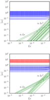Fig. B.1.

Angular frequency |ω_i| of MAC modes, as a function of Le in spheres (β₀ = 0), stratified under gravitational potential (5). The background (toroidal) magnetic field is B₀ = 0.1[−z 1_y+y 1_z] + [−y 1_x+x 1_y] in dimensionless form. From bottom to top: green circles are slow MC and torsional modes (respectively ω_i ∝ Le² and ω_i ∝ Le), blue squares represent fast MC modes and red stars are gravito-inertial modes. The truncation polynomial degree is n = 5. Top panel: neutral fluid (N₀/Ω_s = 0). Bottom panel: stratified fluid (N₀/Ω_s = 10).

Then, we show the spectrum of MAC modes in stratified fluids in the bottom panel of Fig. B.1. The aforementioned hydromagnetic modes still exist in stably stratified interiors, yielding fast and slow MAC waves. However, their properties in the presence of buoyancy and magnetic fields are rather complex in spherical-like domains (Friedlander 1987). On the one hand, fast MAC modes and gravito-inertial modes are barely modified by magnetic fields, as illustrated in Fig. B.1 (bottom panel) when Le ≪ 1. However, they strongly depend on stratification (Friedlander & Siegmann 1982b). On the other hand, slow MC modes can be strongly affected by the magnetic field and stratification (Friedlander 1987). Finally, the buoyancy force also sustains high frequency internal gravity modes. They can be affected by rotation, yielding gravito-inertial modes (Friedlander & Siegmann 1982b).

Appendix C: Mixed resonances of MAC waves

We investigate the possible nonlinear couplings of hydromagnetic waves for tidal instability. We use the same dimensionless variables as in the main text. Resonance condition (12) can only be satisfied if tidal instability involves fast MAC waves (that is inertial or gravito-inertial waves), coupled with either fast or Magneto-Coriolis (slow MC) waves (Kerswell 1993a, 1994). Indeed, in the astrophysical regime Le ≪ 1, the illustrative spectrum in Fig. B.1 clearly shows that no triadic couplings are effective in ellipsoids between two slow MC waves when 1 ≤ Ω₀ ≤ 3. Thus, the couplings of slow MC waves with the equilibrium tidal flow cannot be advocated in stellar interiors.

Second, the mixed couplings between slow and fast hydromagnetic waves is not forbidden in diffusionless fluids. In the weak field regime Le ≪ 1, Kerswell (1993a, 1994) showed that the typical diffusionless growth rate of tidal instability involving mixed couplings scales as (in dimensionless form)

$\begin{matrix} σ \propto L e^{4} β_{0} . \end{matrix}$ $\begin{aligned} \sigma \propto Le^4 \beta _0. \end{aligned}$ (C.1)

However, this diffusionless growth rate must be larger than the (laminar) Joule damping rate of the slow MC waves, that is τ_Ω ∝ −Em |k₀|² in the local theory (Rincon & Rieutord 2003; Sreenivasan & Narasimhan 2017). This gives the typical upper bound on the wave vector

$\begin{matrix} | k_{0} |^{2} ≪ \frac{L e^{4}}{Em} β_{0} . \end{matrix}$ $\begin{aligned} |\boldsymbol{k}_0|^2 \ll \frac{Le^4}{Em} \, \beta _0. \end{aligned}$ (C.2)

In short-period binaries, the typical value for the equatorial ellipticity is β₀ ∼ 10⁻³ − 10⁻² (see Table 2). As given in Table 1, we have also the typical numbers Em ≤ 10⁻¹⁰ and Le ≤ 10⁻⁴. Then, condition (C.2) gives the upper bound |k₀| ≪ 1. This is incompatible with the short-wavelength stability theory, which requires |k₀| ≫ 1. Physically, this shows that the (laminar) Joule damping rate is always larger than the diffusionless growth rate in non-ideal fluids, for any resonance involving slow MC waves in the regime Le ≪ 1. Therefore, mixed couplings of fast/slow waves can be discarded for tidal instability in realistic stellar interiors.

Appendix D: Weakly eccentric synchronised orbits

D.1. Libration forcing

We consider synchronous stratified binary systems moving on weakly eccentric coplanar orbits. Note that the following results are also relevant for (stratified) moons or gaseous planets orbiting around a massive central body (e.g. Kerswell & Malkus 1998; Cébron et al. 2012a; Lemasquerier et al. 2017). We consider a diffusionless tidal model of the tidally deformed fluid body, characterised by an equatorial ellipticity β₀. The fluid body is rotating at the uniform angular velocity Ω_s, aligned in the inertial frame with the orbital angular velocity of the companion along 1_z. We use the dimensionless variables introduced in Sect. 2, that is taking (Ω_s)⁻¹ as the relevant timescale. Due to the weak orbital eccentricity e ≪ 1, the orbital angular velocity has periodic time variations. For the sake of generality, we assume that the tidal forcing has the following (dimensionless) expression, at the leading order in the eccentricity

$\begin{matrix} Ω_{0} (t) = 1 + ϵ_{l} cos (f t), \end{matrix}$ $\begin{aligned} \Omega _0 (t) = 1 + \epsilon _{\rm l} \cos \left( f t \right), \end{aligned}$ (D.1)

where f is the dimensionless frequency of the forcing and ϵ_l ≤ 2e the dimensionless amplitude. Forcing (D.1) is known as longitudinal librations. For this tidal forcing, the equilibrium tidal velocity field has the following form in the central frame

$\begin{matrix} U_{0} (r, t) = - ϵ_{l} cos (f t) [- (1 + β_{0}) y 1_{x} + (1 - β_{0}) x 1_{y}] . \end{matrix}$ $\begin{aligned} \boldsymbol{U}_0 (\boldsymbol{r},t) = - \epsilon _{\rm l} \cos (ft) \, \left[-(1+\beta _0) { y} \, \boldsymbol{1}_x + (1-\beta _0)x \, \boldsymbol{1}_{ y} \right]. \end{aligned}$ (D.2)

Tidal flow (D.2) is prone to libration-driven elliptical instability (LDEI), which is quite similar to tidal instability in non-synchronised systems (e.g. Kerswell & Malkus 1998; Cébron et al. 2012a; Vidal & Cébron 2017; Le Reun & Favier 2019).

D.2. Resonance condition of the LDEI

LDEI is a fluid instability due to sub-harmonic resonances between two waves of angular frequency |ω_i| interacting with basic flow (D.2). By analogy with formula (13) in non-synchronised systems, the sub-harmonic resonance condition becomes

$\begin{matrix} | ω_{i} | = f / 2 . \end{matrix}$ $\begin{aligned} |\omega _i| = f/2. \end{aligned}$ (D.3)

The four kinds of waves [ℋ₁, ℋ₂, ℰ₁, ℰ₂], introduced Sect. 3.2, can be nonlinearly coupled in the instability mechanism. We show the nature of the waves satisfying condition (D.3) in Fig. D.1.

The classical allowable range of LDEI is 0 ≤ f ≤ 4 (e.g. Cébron et al. 2012c), in which only triadic couplings of inertia-gravity waves [ℋ₁, ℋ₂] are involved. In this frequency range, the instability is trapped along critical latitudes for strong enough stratification when N₀/Ω_s ≫ 1. Similar to the non-synchronised configurations, it turns out that the largest growth rate is unaffected by the ratio N₀/Ω_s on these critical latitudes. Thus, they are predicted by the diffusionless formula obtained in neutral fluids (see formula (4) in Cébron et al. 2012c).

In the other frequency range f > 4, LDEI is only due to triadic couplings of internal-gravity waves [ℰ₁, ℰ₂] modified by rotation. Moreover, the instability only exists for strong enough stratification (N₀/Ω_s ≫ 1).

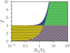Fig. D.1.

Waves at sub-harmonic resonance condition (D.3) for synchronised systems, as a function of (dimensionless) forcing frequency f and N₀/Ω_s. The other notations are identical to the ones introduced in the main text. White regions: no compatible waves satisfying (D.3). Stars (yellow area): hyperbolic waves ℋ₁. Right slash (purple area): hyperbolic waves ℋ₂. Dots (green area): elliptic waves ℰ₁. Back slash (blue area): elliptic waves ℰ₂. The classical allowable region of the instability is 0 ≤ f ≤ 4 in neutral fluids.

D.3. Asymptotic growth rates of the LDEI

As in Sects. 3.2.3 and 3.2.4, the local stability analysis provides analytical expressions of the diffusionless growth rates in the equatorial plane and on the rotation (polar) axis. In the equatorial plane, the resonance condition (D.3) becomes

$\begin{matrix} \sqrt{4 + {\tilde{N}}_{0}^{2} x_{0}^{2}} cos θ_{0} = \pm \frac{f}{2}, \end{matrix}$ $\begin{aligned} \sqrt{4+ \widetilde{N}_0^2 x_0^2} \, \, \cos \theta _0 = \pm \frac{f}{2}, \end{aligned}$ (D.4)

whereas on the rotation axis we have

$\begin{matrix} \sqrt{4 {cos}^{2} θ_{0} + {\tilde{N}}_{0}^{2} x_{0}^{2} {sin}^{2} θ_{0}} = \pm \frac{f}{2} \cdot \end{matrix}$ $\begin{aligned} \sqrt{4\, \cos ^2 \theta _0+ \widetilde{N}_0^2 x_0^2 \sin ^2 \theta _0} \, \, = \pm \frac{f}{2}\cdot \end{aligned}$ (D.5)

Then, the diffusionless growth rate in the equatorial plane is

$\begin{matrix} σ = (1 + \frac{f^{2}}{16}) \frac{| β_{0} - {\tilde{N}}_{0}^{2} x_{0}^{2} (β_{0} - β_{1}) |}{4 + {\tilde{N}}_{0}^{2} x_{0}^{2}} ϵ_{l} \end{matrix}$ $\begin{aligned} \sigma = \left(1+\frac{f^2}{16} \right) \frac{|\beta _0-\widetilde{N}_0^2 x_0^2 (\beta _0-\beta _1)| }{4+ \widetilde{N}_0^2 x_0^2 }\, \epsilon _{\rm l} \end{aligned}$ (D.6)

for a general baroclinic background state β₀ ≠ β₁. On the rotation axis, the diffusionless growth rate is given by

$\begin{matrix} σ = \frac{(16 + f^{2}) (1 - 4 {\tilde{N}}_{0}^{2} x_{0}^{2} f^{- 2})}{16 (4 - {\tilde{N}}_{0}^{2} x_{0}^{2})} β_{0} ϵ_{l} . \end{matrix}$ $\begin{aligned} \sigma = \frac{(16+f^2)(1-4 \widetilde{N}_0^2 x_0^2 f^{-2})}{16 \, (4- \widetilde{N}_0^2 x_0^2 )} \, \beta _0 \epsilon _{\rm l} . \end{aligned}$ (D.7)

Naturally, we recover Eq. (4) of Cébron et al. (2012c), obtained for neutral fluids ( ${\tilde{N}}_{0} = 0$ $\widetilde{N}_0=0$ ). Note that Eq. (25) of Cébron et al. (2013), obtained in the equatorial plane for a buoyancy force of the order β₀, is not recovered by Eq. (D.6). Indeed, their Eq. (25) is approximate because they artificially set θ₀ to its hydrodynamic value 2cos θ₀ = ±f/2, instead of using its exact value given by Eq. (D.4). Finally, by analogy with the arguments given in the main text for non-synchronised systems, the largest diffusionless growth rate in the stellar interior will be insensitive to the strength of stratification, yielding the value for neutral fluids (Cébron et al. 2012c, 2013; Vidal & Cébron 2017) recovered in formula (D.6) when ${\tilde{N}}_{0} = 0$ $\widetilde{N}_0=0$ .

Note finally that formula (30b) also provides exactly the Joule damping rate of the LDEI in neutral fluids ( ${\tilde{N}}_{0} = 0$ $\widetilde{N}_0=0$ ). Besides, formulas of Cébron et al. (2012a,b) are recovered in the limit |k₀| ≫ 1 by using the LDEI resonance condition to set θ₀, that is cos θ₀ = ±f/4 when ${\tilde{N}}_{0} = 0$ $\widetilde{N}_0=0$ .

D.4. Mixing-length theory

We can build a mixing-length theory to get a phenomenological prescription of the turbulent mixing in weakly eccentric synchronised orbits, by analogy with non-synchronised orbits. The main difference with non-synchronised systems is that the typical turbulent velocity u_t should scale as (Favier et al. 2015; Grannan et al. 2016)

$\begin{matrix} u_{t} \propto α_{1} ϵ_{l} β_{0} r_{l} Ω_{s} . \end{matrix}$ $\begin{aligned} u_\mathrm{ t} \propto \alpha _1 \epsilon _{\rm l} \beta _0 r_\mathrm{ l} \, \Omega _\mathrm{ s}. \end{aligned}$ (D.8)

Then, the turbulent prescription becomes

$\begin{matrix} τ_{t} \propto \frac{K_{α}}{ϵ_{l}^{2} β_{0}^{2} Ω_{s}} \end{matrix}$ $\begin{aligned} \tau _\mathrm{ t} \propto \frac{K_\alpha }{\epsilon _{\rm l}^2 \beta _0^2 \, \Omega _\mathrm{ s}} \end{aligned}$ (D.9)

with the numerical pre-factor K_α ∼ 30–50 as in formula (49), which is based on the numerical pre-factors of formulas (41). Hence, the timescale for the turbulent Ohmic diffusion of the fossil field ought to be reduced in synchronised systems (compared to non-synchronised ones) by using formula (D.9).

All Tables

Table 1.

Typical values of dimensionless numbers for stellar interiors. CZ: stellar convective zones, e.g. in the Sun (Charbonneau 2014). RZ: (rapidly) rotating radiative zones (e.g. Rieutord 2006).

In the text

Table 2.

Physical and orbital characteristics of non-synchronised and non-magnetic binary systems, surveyed by the BinaMIcS Collaboration (Alecian et al., in prep.).

In the text

Table 3.

Predictions of tidal scenario for (non-magnetic) close binaries described in Table 2.

In the text

Table 4.

Physical and orbital characteristics of magnetic binary systems surveyed by the BinaMIcS Collaboration (Folsom et al. 2013; Shultz et al. 2015, 2017, 2018).

In the text

All Figures

	Fig. 1. Sketch of idealised orbital configuration between primary body of mass M₁ and secondary one of mass M₂. View from above in the inertial frame. Coplanar and aligned spin and orbital angular velocities [Ω_s, Ω_orb].
In the text

Fig. 2.

Domains of existence of sub-harmonic resonances (13), as a function of Ω₀ = Ω_orb/Ω_s and N₀/Ω_s. In white regions, no waves can satisfy sub-harmonic resonance condition (13). Stars (yellow area): hyperbolic waves ℋ₁. Right slash (purple area): hyperbolic waves ℋ₂. Dots (green area): elliptic waves ℰ₁. Back slash (blue area): elliptic waves ℰ₂. The classical allowable region of tidal instability (for neutral fluids) is −1 ≤ Ω₀ < 3. wave-like domains [ℋ₁, ℋ₂] are illustrated in Fig. 3. Similarly, wave-like domains [ℰ₁, ℰ₂] are illustrated in Fig. 4.

In the text

Fig. 3.

Wave-like domains and colatitude θ₀ (degrees) for waves with hyperbolic turning surfaces ℋ satisfying sub-harmonic resonance condition (13). Left panel: ℋ₁ wave: Ω₀ = 0, N₀/Ω_s = 0.5. Right panel: ℋ₂ wave: Ω₀ = 0, N₀/Ω_s = 2. Dashed grey hyperbolic curve is given by Eq. (14). Tilted dashed grey line is the asymptotic curve given by cos θ₀ = |1 − Ω₀|/2. Waves at the sub-harmonic resonance disappear along the polar axis when z ≤ |1 − Ω₀|/(N₀/Ω_s).

In the text

Fig. 4.

Wave-like domains and colatitude θ₀ (degrees) for waves with ellipsoidal turning surface ℰ satisfying sub-harmonic resonance condition (13). Left panel: ℰ₁ wave: Ω₀ = 3.4, N₀/Ω_s = 2. Right panel: ℰ₂ wave: Ω₀ = 4, N₀/Ω_s = 10. Dashed grey ellipsoidal curve is given by Eq. (14). Vertical dashed grey line is the asymptotic curve given by $s = \sqrt{| 1 - Ω_{0} |^{2} - 4} / (N_{0} / Ω_{s})$ $s = \sqrt{|1-\Omega_0|^2 - 4}/(N_0/\Omega_\mathrm{ s})$ , where s is the cylindrical radius from the spin axis. Waves satisfying the sub-harmonic resonance condition disappear along the polar axis when z ≤ |1 − Ω₀|/(N₀/Ω_s).

In the text

Fig. 5.

Growth rate σ of tidal instability, predicted by formula (23) in equatorial plane (x₀ = 0.5, z₀ = 0), as a function of N₀/Ω_s and Ω₀. Colour bar shows the normalised ratio log₁₀(σ/β₀). White areas correspond to marginally stable areas. For neutral fluids, tidal instability is restricted to the allowable range −1 ≤ Ω₀ ≤ 3 when β₀ ≪ 1. When Ω₀ = 1 (horizontal white line), the basic state is synchronised (see Appendix D).

In the text

Fig. 6.

Largest normalised growth rate σ/β₀ for several configurations, computed with SWAN for equatorial ellipticity β₀ = 0.2. Visualisations in a meridional section using the normalised axes x/a and z/c, with $a = \sqrt{1 + β_{0}}$ $a=\sqrt{1+\beta_0}$ , $b = \sqrt{1 - β_{0}}$ $b=\sqrt{1-\beta_0}$ , and c = 1/(ab). White dashed lines, given by formula (18), show the critical latitudes on which the growth rate is maximum as predicted by (24). For each case, the type of waves involved in parametric mechanism is specified between brackets. Dashed (grey) curves illustrate the domain of existence of ℋ₂ waves at the resonance (in the regime β₀ ≪ 1).

In the text

Fig. 7.

Dimensionless Joule damping −τ_Ω/|1 − Ω₀| of tidal instability (solid blue line), as a function of magnitude |k₀|. Dashed magenta line is given by formula (31), delimiting the two hydromagnetic regimes. Red shaded areas show the typical strength of the diffusionless growth rate of tidal instability σ ∼ 𝒪(β₀), with β₀ ∈ [10⁻⁴, 10⁻²] for close binaries. Computations at Le = 10⁻⁵ and Ek/Pm = 10⁻¹² for the dimensionless fossil field B₀ = 1_z aligned with the spin axis.

In the text

Fig. 8.

Turbulent diffusion of magnetic field by tidal instability, as a function of equatorial ellipticity β₀. Ratio σ_η/|σ_Ω|, with σ_η the global decay rate (44) and σ_Ω the free decay rate (46) without tides. Simulations at Ω₀ = 0, Ek = 10⁻⁴, Pr = 1 and Pm = 0.1. Solid lines are the least-squares fits. Top panel: weakly stratified regime (N₀/Ω_s = 0), with σ_η/|σ_Ω|= − 3.09 β₀ − 1.00. Bottom panel: strongly stratified regime (N₀/Ω_s = 10) with $σ_{η} / | σ_{Ω} | = - 3.13 β_{0}^{2} - 1.21$ $\sigma_\eta/|\sigma_\Omega| = -3.13 \, \beta_0^2 -1.21$ .

In the text

	Fig. 9. Anisotropic turbulent diffusion, generated by tidal instability, of poloidal (dotted) and toroidal (dashed) field lines of fossil field B₀. A possible innermost convective core is represented.
In the text

Fig. 10.

Turbulent magnetic decay τ_t (49) of fossil fields, normalised by laminar Ohmic timescale τ_Ω ∼ (Ω_s Ek/Pm)⁻¹, as a function of equatorial ellipticity β₀ and dimensionless orbital angular frequency Ω₀ = Ω_orb/Ω_s. Non-magnetic close binaries are illustrated by the symbols given in Table 2. Large (white) symbols refer to body 1 of the considered binary, whereas small (cyan) symbols refer to body 2. Computations at Ek/Pm = 10⁻¹² and K_α = 30.

In the text

Fig. B.1.

Angular frequency |ω_i| of MAC modes, as a function of Le in spheres (β₀ = 0), stratified under gravitational potential (5). The background (toroidal) magnetic field is B₀ = 0.1[−z 1_y+y 1_z] + [−y 1_x+x 1_y] in dimensionless form. From bottom to top: green circles are slow MC and torsional modes (respectively ω_i ∝ Le² and ω_i ∝ Le), blue squares represent fast MC modes and red stars are gravito-inertial modes. The truncation polynomial degree is n = 5. Top panel: neutral fluid (N₀/Ω_s = 0). Bottom panel: stratified fluid (N₀/Ω_s = 10).

In the text

Fig. D.1.

Waves at sub-harmonic resonance condition (D.3) for synchronised systems, as a function of (dimensionless) forcing frequency f and N₀/Ω_s. The other notations are identical to the ones introduced in the main text. White regions: no compatible waves satisfying (D.3). Stars (yellow area): hyperbolic waves ℋ₁. Right slash (purple area): hyperbolic waves ℋ₂. Dots (green area): elliptic waves ℰ₁. Back slash (blue area): elliptic waves ℰ₂. The classical allowable region of the instability is 0 ≤ f ≤ 4 in neutral fluids.

In the text

Current usage metrics show cumulative count of Article Views (full-text article views including HTML views, PDF and ePub downloads, according to the available data) and Abstracts Views on Vision4Press platform.

Data correspond to usage on the plateform after 2015. The current usage metrics is available 48-96 hours after online publication and is updated daily on week days.

Initial download of the metrics may take a while.

[1] Abt, H. A., Conti, P. S., Deutsch, A. J., & Wallerstein, G. 1968, ApJ, 153, 177 [NASA ADS] [CrossRef] [Google Scholar]

[2] Akgün, T., Reisenegger, A., Mastrano, A., & Marchant, P. 2013, MNRAS, 433, 2445 [NASA ADS] [CrossRef] [Google Scholar]

[3] Aldridge, K., Seyed-Mahmoud, B., Henderson, G., & van Wijngaarden, W. 1997, Phys. Earth Planet. Inter., 103, 365 [NASA ADS] [CrossRef] [Google Scholar]

[4] Alecian, E., Neiner, C., Wade, G. A., et al. 2014a, Proc. Int. Astron. Union, 9, 330 [CrossRef] [Google Scholar]

[5] Alecian, E., Kochukhov, O., Petit, V., et al. 2014b, A&A, 567, A28 [NASA ADS] [CrossRef] [EDP Sciences] [Google Scholar]

[6] Alecian, E., Tkachenko, A., Neiner, C., Folsom, C. P., & Leroy, B. 2016, A&A, 589, A47 [NASA ADS] [CrossRef] [EDP Sciences] [Google Scholar]

[7] Alecian, E., Villebrun, F., Grunhut, J., et al. 2019, EAS Publ. Ser., 82, 345 [CrossRef] [Google Scholar]

[8] Arlt, R., Hollerbach, R., & Rüdiger, G. 2003, A&A, 401, 1087 [NASA ADS] [CrossRef] [EDP Sciences] [Google Scholar]

[9] Auriere, M., Wade, G. A., Silvester, J., et al. 2007, A&A, 475, 1053 [NASA ADS] [CrossRef] [EDP Sciences] [Google Scholar]

[10] Babcock, H. W. 1958, ApJS, 3, 141 [NASA ADS] [CrossRef] [Google Scholar]

[11] Backus, G., & Rieutord, M. 2017, Phys. Rev. E, 95, 053116 [NASA ADS] [CrossRef] [Google Scholar]

[12] Bajer, K., & Mizerski, K. 2013, Phys. Rev. Lett., 110, 104503 [NASA ADS] [CrossRef] [Google Scholar]

[13] Barker, A. J. 2016, MNRAS, 459, 939 [NASA ADS] [CrossRef] [Google Scholar]

[14] Barker, A. J., & Lithwick, Y. 2013a, MNRAS, 437, 305 [Google Scholar]

[15] Barker, A. J., & Lithwick, Y. 2013b, MNRAS, 437, 305 [Google Scholar]

[16] Barker, A. J., Braviner, H. J., & Ogilvie, G. I. 2016, MNRAS, 459, 924 [NASA ADS] [CrossRef] [Google Scholar]

[17] Bayly, B. J. 1986, Phys. Rev. Lett., 57, 2160 [NASA ADS] [CrossRef] [Google Scholar]

[18] Billant, P., & Chomaz, J.-M. 2001, Phys. Fluids, 13, 1645 [NASA ADS] [CrossRef] [MathSciNet] [Google Scholar]

[19] Blazère, A., Neiner, C., & Petit, P. 2016, MNRAS, 459, L81 [NASA ADS] [CrossRef] [Google Scholar]

[20] Borra, E. F., Landstreet, J. D., & Mestel, L. 1982, ARA&A, 20, 191 [Google Scholar]

[21] Braithwaite, J. 2006, A&A, 449, 451 [NASA ADS] [CrossRef] [EDP Sciences] [Google Scholar]

[22] Braithwaite, J., & Cantiello, M. 2012, MNRAS, 428, 2789 [Google Scholar]

[23] Braithwaite, J., & Nordlund, Å. 2006, A&A, 450, 1077 [NASA ADS] [CrossRef] [EDP Sciences] [Google Scholar]

[24] Braithwaite, J., & Spruit, H. C. 2004, Nature, 431, 819 [NASA ADS] [CrossRef] [PubMed] [Google Scholar]

[25] Braithwaite, J., & Spruit, H. C. 2017, R. Soc. Open Sci., 4, 160271 [Google Scholar]

[26] Brethouwer, G., Billant, P., Lindborg, E., & Chomaz, J.-M. 2007, J. Fluid Mech., 585, 343 [NASA ADS] [CrossRef] [Google Scholar]

[27] Brun, A. S., Browning, M. K., & Toomre, J. 2005, ApJ, 629, 461 [NASA ADS] [CrossRef] [Google Scholar]

[28] Brunet, M., Dauxois, T., & Cortet, P.-P. 2019, Phys. Rev. Fluids, 4, 034801 [NASA ADS] [CrossRef] [Google Scholar]

[29] Busse, F. H. 1981, Geophys. Astrophys. Fluid Dyn., 17, 215 [NASA ADS] [CrossRef] [Google Scholar]

[30] Busse, F. H. 1982, ApJ, 259, 759 [NASA ADS] [CrossRef] [Google Scholar]

[31] Caleo, A., & Balbus, S. A. 2016, MNRAS, 457, 1711 [NASA ADS] [CrossRef] [Google Scholar]

[32] Carrier, F., North, P., Udry, S., & Babel, J. 2002, A&A, 394, 151 [NASA ADS] [CrossRef] [EDP Sciences] [Google Scholar]

[33] Cattaneo, F. 1994, ApJ, 434, 200 [NASA ADS] [CrossRef] [Google Scholar]

[34] Cattaneo, F., & Vainshtein, S. I. 1991, ApJ, 376, L21 [NASA ADS] [CrossRef] [Google Scholar]

[35] Cébron, D., & Hollerbach, R. 2014, ApJ, 789, L25 [Google Scholar]

[36] Cébron, D., Le Bars, M., Le Gal, P., et al. 2013, Icarus, 226, 1642 [NASA ADS] [CrossRef] [Google Scholar]

[37] Cébron, D., Le Bars, M., Moutou, C., & Le Gal, P. 2012a, A&A, 539, A78 [NASA ADS] [CrossRef] [EDP Sciences] [Google Scholar]

[38] Cébron, D., Le Bars, M., Maubert, P., & Le Gal, P. 2012b, Geophys. Astrophys. Fluid Dyn., 106, 524 [NASA ADS] [CrossRef] [Google Scholar]

[39] Cébron, D., Le Bars, M., Noir, J., & Aurnou, J. M. 2012c, Phys. Fluids, 24, 061703 [NASA ADS] [CrossRef] [Google Scholar]

[40] Cébron, D., Maubert, P., & Le Bars, M. 2010, Geophys. J. Int., 182, 1311 [Google Scholar]

[41] Chandrasekhar, S. 1969, Ellipsoidal Figures of Equilibrium (London: Yale Univiversity Press) [Google Scholar]

[42] Charbonneau, P. 2014, ARA&A, 52, 251 [Google Scholar]

[43] Clausen, N., & Tilgner, A. 2014, A&A, 562, A25 [NASA ADS] [CrossRef] [EDP Sciences] [Google Scholar]

[44] Clausen, J. V., Olsen, E. H., Helt, B. E., & Claret, A. 2010, A&A, 510, A91 [NASA ADS] [CrossRef] [EDP Sciences] [Google Scholar]

[45] Commerçon, B., Hennebelle, P., Audit, E., Chabrier, G., & Teyssier, R. 2010, A&A, 510, L3 [NASA ADS] [CrossRef] [EDP Sciences] [Google Scholar]

[46] Commerçon, B., Hennebelle, P., & Henning, T. 2011, ApJ, 742, L9 [NASA ADS] [CrossRef] [Google Scholar]

[47] Craik, A. D. D. 1988, Proc. R. Soc. London Ser. A, 417, 235 [NASA ADS] [CrossRef] [Google Scholar]

[48] Craik, A. D. D. 1989, J. Fluid Mech., 198, 275 [NASA ADS] [CrossRef] [Google Scholar]

[49] Craik, A. D. D., & Criminale, W. O. 1986, Proc. R. Soc. London Ser. A, 406, 13 [NASA ADS] [CrossRef] [Google Scholar]

[50] Değgirmenc, Ö. L. 1997, Space Sci., 253, 237 [NASA ADS] [CrossRef] [Google Scholar]

[51] Dintrans, B., Rieutord, M., & Valdettaro, L. 1999, J. Fluid Mech., 398, 271 [NASA ADS] [CrossRef] [Google Scholar]

[52] Dubrulle, B., & Frisch, U. 1991, Phys. Rev. A, 43, 5355 [NASA ADS] [CrossRef] [MathSciNet] [PubMed] [Google Scholar]

[53] Duez, V., & Mathis, S. 2010, A&A, 517, A58 [NASA ADS] [CrossRef] [EDP Sciences] [Google Scholar]

[54] Duez, V., Braithwaite, J., & Mathis, S. 2010, ApJ, 724, L34 [Google Scholar]

[55] Edelmann, P. V. F., Ratnasingam, R. P., Pedersen, M. G., et al. 2019, ApJ, 876, 4 [NASA ADS] [CrossRef] [Google Scholar]

[56] Eloy, C., & Le Dizès, S. 1999, J. Fluid Mech., 378, 145 [NASA ADS] [CrossRef] [Google Scholar]

[57] Elstner, D., & Rüdiger, G. 2007, Astron. Nachr., 328, 1130 [NASA ADS] [CrossRef] [Google Scholar]

[58] Fabijonas, B. R. 2002, Phys. Plasmas, 9, 3359 [NASA ADS] [CrossRef] [Google Scholar]

[59] Favier, B., Grannan, A. M., Le Bars, M., & Aurnou, J. M. 2015, Phys. Fluids, 27, 066601 [NASA ADS] [CrossRef] [Google Scholar]

[60] Featherstone, N. A., Browning, M. K., Brun, A. S., & Toomre, J. 2009, ApJ, 705, 1000 [NASA ADS] [CrossRef] [Google Scholar]

[61] Folsom, C. P., Likuski, K., Wade, G. A., et al. 2013, MNRAS, 431, 1513 [NASA ADS] [CrossRef] [Google Scholar]

[62] Friedlander, S. 1987, Geophys. Astrophys. Fluid Dyn., 39, 315 [NASA ADS] [CrossRef] [Google Scholar]

[63] Friedlander, S. 1989, Geophys. Astrophys. Fluid Dyn., 48, 53 [NASA ADS] [CrossRef] [Google Scholar]

[64] Friedlander, S., & Siegmann, W. L. 1982a, J. Fluid Mech., 114, 123 [NASA ADS] [CrossRef] [MathSciNet] [Google Scholar]

[65] Friedlander, S., & Siegmann, W. L. 1982b, Geophys. Astrophys. Fluid Dyn., 19, 267 [NASA ADS] [CrossRef] [Google Scholar]

[66] Friedlander, S., & Vishik, M. 1990, Geophys. Astrophys. Fluid Dyn., 55, 19 [NASA ADS] [CrossRef] [Google Scholar]

[67] Friedlander, S., & Vishik, M. M. 1991, Phys. Rev. Lett., 66, 2204 [NASA ADS] [CrossRef] [Google Scholar]

[68] Friedlander, S., & Vishik, M. M. 1995, J. Nonlinear Sci., 5, 416 [Google Scholar]

[69] Gagnier, D., & Garaud, P. 2018, ApJ, 862, 36 [NASA ADS] [CrossRef] [Google Scholar]

[70] Garaud, P., Gagnier, D., & Verhoeven, J. 2017, ApJ, 837, 133 [NASA ADS] [CrossRef] [Google Scholar]

[71] Gastine, T., & Dintrans, B. 2008a, A&A, 484, 29 [NASA ADS] [CrossRef] [EDP Sciences] [Google Scholar]

[72] Gastine, T., & Dintrans, B. 2008b, A&A, 490, 743 [NASA ADS] [CrossRef] [EDP Sciences] [Google Scholar]

[73] Giménez, A., & Clausen, J. V. 1994, A&A, 291, 795 [NASA ADS] [Google Scholar]

[74] Giuricin, G., Mardirossian, F., & Mezzetti, M. 1984a, A&A, 135, 393 [NASA ADS] [Google Scholar]

[75] Giuricin, G., Mardirossian, F., & Mezzetti, M. 1984b, A&A, 131, 152 [Google Scholar]

[76] Gledzer, E. B., & Ponomarev, V. M. 1992, J. Fluid Mech., 240, 1 [NASA ADS] [CrossRef] [Google Scholar]

[77] Godeferd, F. S., & Staquet, C. 2003, J. Fluid Mech., 486, 115 [NASA ADS] [CrossRef] [Google Scholar]

[78] Goldreich, P., & Schubert, G. 1967, ApJ, 150, 571 [Google Scholar]

[79] Grannan, A. M., Favier, B., Le Bars, M., & Aurnou, J. M. 2016, Geophys. J. Int., 208, 1690 [NASA ADS] [Google Scholar]

[80] Greenspan, H. P. 1968, The Theory of Rotating Fluids (Cambridge: Cambridge University Press) [Google Scholar]

[81] Groenewegen, M. A. T., Decin, L., Salaris, M., & De Cat, P. 2007, A&A, 463, 579 [NASA ADS] [CrossRef] [EDP Sciences] [Google Scholar]

[82] Grunhut, J. H., Wade, G. A., Neiner, C., et al. 2016, MNRAS, 465, 2432 [Google Scholar]

[83] Gubbins, D., & Roberts, P. H. 1987, Geomagnetism, 2, 1 [Google Scholar]

[84] Guermond, J.-L., Léorat, J., Luddens, F., & Nore, C. 2013, Eur. J. Mech. B Fluids, 39, 1 [NASA ADS] [CrossRef] [Google Scholar]

[85] Herreman, W., Cébron, D., Le Dizès, S., & Le Gal, P. 2010, J. Fluid Mech., 661, 130 [NASA ADS] [CrossRef] [Google Scholar]

[86] Herreman, W., Le Bars, M., & Le Gal, P. 2009, Phys. Fluids, 21, 046602 [NASA ADS] [CrossRef] [Google Scholar]

[87] Heyvaerts, J., & Priest, E. 1983, A&A, 117, 220 [NASA ADS] [Google Scholar]

[88] Hubrig, S., Fossati, L., Carroll, T. A., et al. 2014, A&A, 564, L10 [NASA ADS] [CrossRef] [EDP Sciences] [Google Scholar]

[89] Hut, P. 1981, A&A, 99, 126 [NASA ADS] [Google Scholar]

[90] Hut, P. 1982, A&A, 110, 37 [Google Scholar]

[91] Ivers, D. 2017, Geophys. Astrophys. Fluid Dyn., 111, 333 [NASA ADS] [CrossRef] [Google Scholar]

[92] Jouve, L., & Ogilvie, G. I. 2014, J. Fluid Mech., 745, 223 [Google Scholar]

[93] Jouve, L., Gastine, T., & Lignières, F. 2015, A&A, 575, A106 [NASA ADS] [CrossRef] [EDP Sciences] [Google Scholar]

[94] Kaiser, R., & Busse, F. 2017, Geophys. Astrophys. Fluid Dyn., 111, 355 [NASA ADS] [CrossRef] [Google Scholar]

[95] Käpylä, P. J., Rheinhardt, M., Brandenburg, A., & Käpylä, M. J. 2019, A&A, submitted [arXiv:1901.00787] [Google Scholar]

[96] Kerswell, R. 1994, J. Fluid Mech., 274, 219 [NASA ADS] [CrossRef] [Google Scholar]

[97] Kerswell, R. R. 1993a, Geophys. Astrophys. Fluid Dyn., 71, 105 [NASA ADS] [CrossRef] [Google Scholar]

[98] Kerswell, R. R. 1993b, Geophys. Astrophys. Fluid Dyn., 72, 107 [NASA ADS] [CrossRef] [MathSciNet] [Google Scholar]

[99] Kerswell, R. R. 2002, Annu. Rev. Fluid Mech., 34, 83 [NASA ADS] [CrossRef] [MathSciNet] [Google Scholar]

[100] Kerswell, R. R., & Malkus, W. V. R. 1998, Geophys. Res. Lett., 25, 603 [NASA ADS] [CrossRef] [Google Scholar]

[101] Kippenhahn, R., Weigert, A., & Weiss, A. 1990, Stellar Structure and Evolution (Berlin: Springer), 282 [Google Scholar]

[102] Kirillov, O. N., & Mutabazi, I. 2017, J. Fluid Mech., 818, 319 [NASA ADS] [CrossRef] [Google Scholar]

[103] Kirillov, O. N., Stefani, F., & Fukumoto, Y. 2014, J. Fluid Mech., 760, 591 [NASA ADS] [CrossRef] [Google Scholar]

[104] Kitchatinov, L. L. 2014, ApJ, 784, 81 [NASA ADS] [CrossRef] [Google Scholar]

[105] Kitchatinov, L. L., Pipin, V. V., & Rüdiger, G. 1994, Astron. Nachr., 315, 157 [NASA ADS] [CrossRef] [Google Scholar]

[106] Kochukhov, O., Johnston, C., Alecian, E., Wade, G. A., & the BinaMIcS Collaboration 2018, MNRAS, 478, 1749 [NASA ADS] [CrossRef] [Google Scholar]

[107] Kondić, T., Hughes, D. W., & Tobias, S. M. 2016, ApJ, 823, 111 [NASA ADS] [CrossRef] [Google Scholar]

[108] Labbé, F., Jault, D., & Gillet, N. 2015, Geophys. Astrophys. Fluid Dyn., 109, 587 [NASA ADS] [CrossRef] [Google Scholar]

[109] Lacaze, L., Le Gal, P., & Le Dizes, S. 2004, J. Fluid Mech., 505, 1 [NASA ADS] [CrossRef] [Google Scholar]

[110] Lacaze, L., Le Gal, P., & Le Dizes, S. 2005, Phys. Earth Planet. Inter., 151, 194 [NASA ADS] [CrossRef] [Google Scholar]

[111] Lacaze, L., Ryan, K., & Le Dizes, S. 2007, J. Fluid Mech., 577, 341 [NASA ADS] [CrossRef] [Google Scholar]

[112] Lai, D., Rasio, F. A., & Shapiro, S. L. 1993, ApJS, 88, 205 [NASA ADS] [CrossRef] [Google Scholar]

[113] Landstreet, J. D., Kochukhov, O., Alecian, E., et al. 2017, A&A, 601, A129 [NASA ADS] [CrossRef] [EDP Sciences] [Google Scholar]

[114] Le Bars, M., & Le Dizès, S. 2006, J. Fluid Mech., 563, 189 [NASA ADS] [CrossRef] [Google Scholar]

[115] Le Bars, M., Lacaze, L., Le Dizes, S., Le Gal, P., & Rieutord, M. 2010, Phys. Earth Planet. Inter., 178, 48 [NASA ADS] [CrossRef] [Google Scholar]

[116] Le Dizès, S. 2000, Phys. Fluids, 12, 2762 [NASA ADS] [CrossRef] [Google Scholar]

[117] Le Duc, A. 2001, PhD Thesis, Ecole Centrale de Lyon [Google Scholar]

[118] Le Reun, T., Favier, B., Barker, A. J., & Le Bars, M. 2017, Phys. Rev. Lett., 119, 034502 [NASA ADS] [CrossRef] [Google Scholar]

[119] Le Reun, T., Favier, B., & Le Bars, M. 2018, J. Fluid Mech., 840, 498 [NASA ADS] [CrossRef] [Google Scholar]

[120] Le Reun, T., Favier, B., & Le Bars, M. 2019, J. Fluid Mech., accepted [arXiv:1907.10907] [Google Scholar]

[121] Lebovitz, N. R. 1989, Geophys. Astrophys. Fluid Dyn., 46, 221 [NASA ADS] [CrossRef] [Google Scholar]

[122] Lebovitz, N., & Lifschitz, A. 1992, Proc. R. Soc. London Ser. A, 438, 265 [NASA ADS] [CrossRef] [Google Scholar]

[123] Lebovitz, N. R., & Zweibel, E. 2004, ApJ, 609, 301 [NASA ADS] [CrossRef] [Google Scholar]

[124] Lehnert, B. 1954, ApJ, 119, 647 [NASA ADS] [CrossRef] [Google Scholar]

[125] Lemasquerier, D., Grannan, A. M., Vidal, J., et al. 2017, J. Geophys. Res.: Planets, 122, 1926 [NASA ADS] [CrossRef] [Google Scholar]

[126] Lifschitz, A., & Hameiri, E. 1991, Phys. Fluids, 3, 2644 [NASA ADS] [CrossRef] [MathSciNet] [Google Scholar]

[127] Lifschitz, A., & Lebovitz, N. 1993, ApJ, 408, 603 [NASA ADS] [CrossRef] [Google Scholar]

[128] Lignieres, F., Petit, P., Böhm, T., & Auriere, M. 2009, A&A, 500, L41 [NASA ADS] [CrossRef] [EDP Sciences] [Google Scholar]

[129] Lin, Y., & Ogilvie, G. I. 2017, MNRAS, 468, 1387 [NASA ADS] [CrossRef] [Google Scholar]

[130] MacDonald, J., & Mullan, D. J. 2004, MNRAS, 348, 702 [NASA ADS] [CrossRef] [Google Scholar]

[131] MacGregor, K. B., & Cassinelli, J. P. 2003, ApJ, 586, 480 [NASA ADS] [CrossRef] [Google Scholar]

[132] Maffioli, A., & Davidson, P. A. 2016, J. Fluid Mech., 786, 210 [NASA ADS] [CrossRef] [Google Scholar]

[133] Mahy, L., Gosset, E., Sana, H., et al. 2012, A&A, 540, A97 [NASA ADS] [CrossRef] [EDP Sciences] [Google Scholar]

[134] Makaganiuk, V., Kochukhov, O., Piskunov, N., et al. 2011, A&A, 529, A160 [NASA ADS] [CrossRef] [EDP Sciences] [Google Scholar]

[135] Malkus, W. V. R. 1967, J. Fluid Mech., 28, 793 [NASA ADS] [CrossRef] [Google Scholar]

[136] Marti, P., Schaeffer, N., Hollerbach, R., et al. 2014, Geophys. J. Int., 197, 119 [NASA ADS] [CrossRef] [Google Scholar]

[137] Mathis, S., & de Brye, N. 2011, A&A, 526, A65 [NASA ADS] [CrossRef] [EDP Sciences] [Google Scholar]

[138] Mathis, S., Palacios, A., & Zahn, J.-P. 2004, A&A, 425, 243 [NASA ADS] [CrossRef] [EDP Sciences] [Google Scholar]

[139] Mathis, S., Neiner, C., & Minh, N. T. 2014, A&A, 565, A47 [NASA ADS] [CrossRef] [EDP Sciences] [Google Scholar]

[140] Mathis, S., Prat, V., Amard, L., et al. 2018, A&A, 620, A22 [NASA ADS] [CrossRef] [EDP Sciences] [Google Scholar]

[141] Mathys, G. 2017, A&A, 601, A14 [NASA ADS] [CrossRef] [EDP Sciences] [Google Scholar]

[142] Matsui, H., Heien, E., Aubert, J., et al. 2016, Geochem. Geophys. Geosyst., 17, 1586 [NASA ADS] [CrossRef] [Google Scholar]

[143] Mazeh, T. 2008, in Tidal Effects in Stars, Planets and Disks, eds. M. J. Goupil, J. P. Zahn, & T. Mazeh, Eur. Astron. Soc. Publ. Ser., 29, 1 [Google Scholar]

[144] Mirouh, G. M., Baruteau, C., Rieutord, M., & Ballot, J. 2016, J. Fluid Mech., 800, 213 [NASA ADS] [CrossRef] [Google Scholar]

[145] Miyazaki, T. 1993, Phys. Fluids, 5, 2702 [NASA ADS] [CrossRef] [Google Scholar]

[146] Miyazaki, T., & Fukumoto, Y. 1991, Phys. Fluids, 3, 606 [NASA ADS] [CrossRef] [Google Scholar]

[147] Miyazaki, T., & Fukumoto, Y. 1992, Phys. Fluids, 4, 2515 [NASA ADS] [CrossRef] [Google Scholar]

[148] Mizerski, K. A., & Bajer, K. 2011, Phys. D, 240, 1629 [CrossRef] [Google Scholar]

[149] Mizerski, K. A., & Lyra, W. 2012, J. Fluid Mech., 698, 358 [NASA ADS] [CrossRef] [Google Scholar]

[150] Mizerski, K. A., Bajer, K., & Moffatt, H. K. 2012, J. Fluid Mech., 707, 111 [NASA ADS] [CrossRef] [Google Scholar]

[151] Moffatt, H. K. 1978, Magnetic Field Generation in Electrically, Conducting Fluids (Cambridge: Cambridge University Press) [Google Scholar]

[152] Moss, D. 1992, MNRAS, 257, 593 [NASA ADS] [Google Scholar]

[153] Moss, D. 2001, Magnetic Fields Across the Hertzsprung-Russell Diagram, 248, 305 [NASA ADS] [Google Scholar]

[154] Nazarenko, S., Kevlahan, N. K.-R., & Dubrulle, B. 1999, J. Fluid Mech., 390, 325 [NASA ADS] [CrossRef] [Google Scholar]

[155] Nduka, A. 1971, ApJ, 170, 131 [NASA ADS] [CrossRef] [Google Scholar]

[156] Nordstrom, B., & Johansen, K. T. 1994, A&A, 282, 787 [NASA ADS] [Google Scholar]

[157] Ogilvie, G. I. 2009, MNRAS, 396, 794 [NASA ADS] [CrossRef] [Google Scholar]

[158] Ogilvie, G. I. 2014, ARA&A, 52, 171 [Google Scholar]

[159] Parker, E. N. 1979, Cosmical Magnetic Fields: Their Origin and Their Activity (Oxford: Oxford University Press) [Google Scholar]

[160] Petit, P., Lignieres, F., Wade, G. A., et al. 2010, A&A, 523, A41 [NASA ADS] [CrossRef] [EDP Sciences] [Google Scholar]

[161] Petit, P., Lignieres, F., Aurière, M., et al. 2011, A&A, 532, L13 [NASA ADS] [CrossRef] [EDP Sciences] [Google Scholar]

[162] Pierrehumbert, R. T. 1986, Phys. Rev. Lett., 57, 2157 [NASA ADS] [CrossRef] [Google Scholar]

[163] Reddy, K. S., Favier, B., & Le Bars, M. 2018, Geophys. Res. Lett., 45, 1741 [NASA ADS] [CrossRef] [Google Scholar]

[164] Reinaud, J. N., Dritschel, D. G., & Koudella, C. R. 2003, J. Fluid Mech., 474, 175 [NASA ADS] [CrossRef] [Google Scholar]

[165] Reisenegger, A. 2009, A&A, 499, 557 [NASA ADS] [CrossRef] [EDP Sciences] [Google Scholar]

[166] Remus, F., Mathis, S., & Zahn, J.-P. 2012, A&A, 544, A132 [NASA ADS] [CrossRef] [EDP Sciences] [Google Scholar]

[167] Rieutord, M. 1992, A&A, 259, 581 [Google Scholar]

[168] Rieutord, M. 2004, Symposium-International Astronomical Union (Cambridge: Cambridge University Press), 215, 394 [NASA ADS] [CrossRef] [Google Scholar]

[169] Rieutord, M. 2006, A&A, 451, 1025 [NASA ADS] [CrossRef] [EDP Sciences] [Google Scholar]

[170] Rieutord, M., & Valdettaro, L. 1997, J. Fluid Mech., 341, 77 [Google Scholar]

[171] Rieutord, M., & Valdettaro, L. 2010, J. Fluid Mech., 643, 363 [NASA ADS] [CrossRef] [Google Scholar]

[172] Rieutord, M., & Valdettaro, L. 2018, J. Fluid Mech., 844, 597 [NASA ADS] [CrossRef] [Google Scholar]

[173] Rieutord, M., & Zahn, J.-P. 1997, ApJ, 474, 760 [Google Scholar]

[174] Rieutord, M., Georgeot, B., & Valdettaro, L. 2000, Phys. Rev. Lett., 85, 4277 [NASA ADS] [CrossRef] [PubMed] [Google Scholar]

[175] Rincon, F., & Rieutord, M. 2003, A&A, 398, 663 [NASA ADS] [CrossRef] [EDP Sciences] [Google Scholar]

[176] Rocca, A. 1987, A&A, 175, 81 [Google Scholar]

[177] Rocca, A. 1989, A&A, 213, 114 [NASA ADS] [Google Scholar]

[178] Rodrigues, S. B. 2017, J. Eng. Math., 106, 1 [CrossRef] [Google Scholar]

[179] Rogers, T. M., & McElwaine, J. N. 2017, ApJ, 848, L1 [NASA ADS] [CrossRef] [Google Scholar]

[180] Rüdiger, G., Gellert, M., Schultz, M., Hollerbach, R., & Stefani, F. 2013, MNRAS, 438, 271 [Google Scholar]

[181] Rüdiger, G., Gellert, M., Spada, F., & Tereshin, I. 2015, A&A, 573, A80 [NASA ADS] [CrossRef] [EDP Sciences] [Google Scholar]

[182] Schaeffer, N. 2013, Geochem. Geophys. Geosyst., 14, 751 [NASA ADS] [CrossRef] [Google Scholar]

[183] Schaeffer, N., Jault, D., Nataf, H.-C., & Fournier, A. 2017, Geophys. J. Int., 211, 1 [NASA ADS] [CrossRef] [Google Scholar]

[184] Schatzman, E. 1993, A&A, 279, 431 [NASA ADS] [Google Scholar]

[185] Schmitt, D. 2010, Geophys. Astrophys. Fluid Dyn., 104, 135 [NASA ADS] [CrossRef] [Google Scholar]

[186] Schneider, F. R. N., Podsiadlowski, P., Langer, N., Castro, N., & Fossati, L. 2016, MNRAS, 457, 2355 [NASA ADS] [CrossRef] [Google Scholar]

[187] Seyed-Mahmoud, B., Henderson, G., & Aldridge, K. 2000, Phys. Earth Planet. Inter., 117, 51 [NASA ADS] [CrossRef] [Google Scholar]

[188] Seyed-Mahmoud, B., Aldridge, K., & Henderson, G. 2004, Phys. Earth Planet. Inter., 142, 257 [NASA ADS] [CrossRef] [Google Scholar]

[189] Shenar, T., Oskinova, L., Hamann, W.-R., et al. 2015, ApJ, 809, 135 [NASA ADS] [CrossRef] [Google Scholar]

[190] Shultz, M., Wade, G. A., Alecian, E., & BinaMIcS 2015, MNRAS, 454, L1 [NASA ADS] [CrossRef] [Google Scholar]

[191] Shultz, M., Rivinius, T., Wade, G. A., et al. 2017, MNRAS, 475, 839 [NASA ADS] [CrossRef] [Google Scholar]

[192] Shultz, M. E., Wade, G. A., Rivinius, T., et al. 2018, MNRAS, 475, 5144 [NASA ADS] [Google Scholar]

[193] Sikora, J., Wade, G. A., Power, J., & Neiner, C. 2018, MNRAS, 483, 3127 [Google Scholar]

[194] Simitev, R. D., & Busse, F. H. 2017, Geophys. Astrophys. Fluid Dyn., 111, 369 [NASA ADS] [CrossRef] [Google Scholar]

[195] Spiegel, E. A., & Veronis, G. 1960, ApJ, 131, 442 [NASA ADS] [CrossRef] [MathSciNet] [Google Scholar]

[196] Spruit, H. C. 1999, A&A, 349, 189 [NASA ADS] [Google Scholar]

[197] Spruit, H. C. 2002, A&A, 381, 923 [NASA ADS] [CrossRef] [EDP Sciences] [Google Scholar]

[198] Sreenivasan, B., & Narasimhan, G. 2017, J. Fluid Mech., 828, 867 [NASA ADS] [CrossRef] [Google Scholar]

[199] Tamajo, E., Munari, U., Siviero, A., Tomasella, L., & Dallaporta, S. 2012, A&A, 539, A139 [NASA ADS] [CrossRef] [EDP Sciences] [Google Scholar]

[200] Tennekes, H., & Lumley, J. L. 1972, A First Course in Turbulence (Cambridge: MIT Press) [Google Scholar]

[201] Tilgner, A. 2004, Geophys. Astrophys. Fluid Dyn., 98, 225 [NASA ADS] [CrossRef] [Google Scholar]

[202] Townsend, A. A. 1958, J. Fluid Mech., 4, 361 [NASA ADS] [CrossRef] [Google Scholar]

[203] Uytterhoeven, K., Harmanec, P., Telting, J. H., & Aerts, C. 2005, A&A, 440, 249 [NASA ADS] [CrossRef] [EDP Sciences] [Google Scholar]

[204] Vainshtein, S. I., & Rosner, R. 1991, ApJ, 376, 199 [NASA ADS] [CrossRef] [Google Scholar]

[205] Vantieghem, S. 2014, Proc. R. Soc. London Ser. A, 470, 20140093 [NASA ADS] [CrossRef] [Google Scholar]

[206] Vidal, J., & Cébron, D. 2017, J. Fluid Mech., 833, 469 [NASA ADS] [CrossRef] [Google Scholar]

[207] Vidal, J., Cébron, D., Schaeffer, N., & Hollerbach, R. 2018, MNRAS, 475, 4579 [NASA ADS] [CrossRef] [Google Scholar]

[208] Wade, G. A., Neiner, C., Alecian, E., et al. 2015, MNRAS, 456, 2 [Google Scholar]

[209] Waite, M. L., & Bartello, P. 2006, J. Fluid Mech., 568, 89 [NASA ADS] [CrossRef] [Google Scholar]

[210] Waleffe, F. 1990, Phys. Fluids A, 2, 76 [NASA ADS] [CrossRef] [MathSciNet] [Google Scholar]

[211] Weinberg, N. N. 2016, ApJ, 819, 109 [NASA ADS] [CrossRef] [Google Scholar]

[212] Wirth, A., Gama, S., & Frisch, U. 1995, J. Fluid Mech., 288, 249 [NASA ADS] [CrossRef] [MathSciNet] [Google Scholar]

[213] Witte, M. G., & Savonije, G. J. 1999, A&A, 350, 129 [NASA ADS] [Google Scholar]

[214] Witte, M. G., & Savonije, G. J. 2001, A&A, 366, 840 [NASA ADS] [CrossRef] [EDP Sciences] [Google Scholar]

[215] Yousef, T. A., Brandenburg, A., & Rüdiger, G. 2003, A&A, 411, 321 [NASA ADS] [CrossRef] [EDP Sciences] [Google Scholar]

[216] Zahn, J.-P. 1966, Ann. Astrophys., 29, 313 [NASA ADS] [Google Scholar]

[217] Zahn, J. P. 1974, Symposium-International Astronomical Union (Cambridge: Cambridge University Press), 59, 185 [NASA ADS] [CrossRef] [Google Scholar]

[218] Zahn, J.-P. 1975, A&A, 41, 329 [NASA ADS] [Google Scholar]

[219] Zahn, J.-P. 1977, A&A, 57, 383 [NASA ADS] [Google Scholar]

[220] Zahn, J.-P. 1992, A&A, 265, 115 [NASA ADS] [Google Scholar]

[221] Zahn, J.-P. 2008, Proc. Int. Astron. Union, 4, 47 [CrossRef] [Google Scholar]

[222] Zhang, K., Liao, X., & Schubert, G. 2003, ApJ, 585, 1124 [NASA ADS] [CrossRef] [Google Scholar]

[223] Zimmerman, M. K., Thompson, S. E., Mullally, F., et al. 2017, ApJ, 846, 147 [NASA ADS] [CrossRef] [Google Scholar]

Fossil field decay due to nonlinear tides in massive binaries

1. Introduction

2. Formulation of the problem

2.1. Assumptions

2.2. Governing equations

2.3. Reference ellipsoidal configuration

3. Onset of tidal instability

3.1. Short-wavelength perturbations

3.2. Asymptotic analysis

3.2.1. Triadic (nonlinear) couplings

3.2.2. Hydrodynamic waves at the parametric resonance

3.2.3. Asymptotic growth rate in the equatorial plane

3.2.4. Along rotation axis

3.3. Numerical solutions in the orbital range −1 ≤ Ω0 ≤ 3

3.4. Leading-order (laminar) diffusive effects

3.5. Other dissipative mechanisms

4. Turbulent mixing due to nonlinear tidal flows

4.1. Assumptions

4.2. Mixing-length theory

4.3. Phenomenological prescriptions

4.3.1. Weakly stratified regime (N0/Ωs ≤ 1)

4.3.2. Stratified regimes (N0/Ωs ≥ 1)

4.4. Validation against numerical simulations

5. Astrophysical discussion

5.1. A new scenario?

5.2. Non-magnetic binaries

5.3. Magnetic binaries

6. Conclusion

6.1. Summary

6.2. Perspectives

Acknowledgments

References

Appendix A: Local (WKB) stability equations

A.1. Linearised stability equations

A.2. Short-wavelength perturbations

A.3. Eulerian stability equations

A.4. Lagrangian equations along fluid trajectories

Appendix B: MAC modes in triaxial ellipsoids

B.1. Assumptions

B.2. Galerkin method

B.3. Hydromagnetic modes

Appendix C: Mixed resonances of MAC waves

Appendix D: Weakly eccentric synchronised orbits

D.1. Libration forcing

D.2. Resonance condition of the LDEI

D.3. Asymptotic growth rates of the LDEI

D.4. Mixing-length theory

All Tables

All Figures

3.3. Numerical solutions in the orbital range −1 ≤ Ω₀ ≤ 3

4.3.1. Weakly stratified regime (N₀/Ω_s ≤ 1)

4.3.2. Stratified regimes (N₀/Ω_s ≥ 1)