| Issue |
A&A
Volume 629, September 2019
|
|
|---|---|---|
| Article Number | A70 | |
| Number of page(s) | 14 | |
| Section | Galactic structure, stellar clusters and populations | |
| DOI | https://doi.org/10.1051/0004-6361/201935264 | |
| Published online | 06 September 2019 | |
The tilt of the velocity ellipsoid in the Milky Way with Gaia DR2
1
Kapteyn Astronomical Institute, University of Groningen, Landleven 12, 9747 Groningen, The Netherlands
e-mail: This email address is being protected from spambots. You need JavaScript enabled to view it.
2
Sterrewacht Leiden, Leiden University, Postbus 9513, 2300 Leiden, The Netherlands
3
Max Planck Institute for Extraterrestrial Physics, Giessenbachstrasse 1, 85748 Garching, Germany
4
Université de Strasbourg, CNRS UMR 7550, Observatoire astronomique de Strasbourg, 11 rue de l’Université, 67000 Strasbourg, France
Received:
13
February
2019
Accepted:
7
August
2019
Abstract
The velocity distribution of stars is a sensitive probe of the gravitational potential of the Galaxy, and hence of its dark matter distribution. In particular, the shape of the dark halo (e.g. spherical, oblate, or prolate) determines velocity correlations, and different halo geometries are expected to result in measurable differences. Here we explore and interpret the correlations in the (vR, vz)-velocity distribution as a function of position in the Milky Way. We selected a high-quality sample of stars from the Gaia DR2 catalogue and characterised the orientation of the velocity distribution or tilt angle over a radial distance range of [4 − 13] kpc and up to 3.5 kpc away from the Galactic plane while taking into account the effects of the measurement errors. We find that the tilt angles change from spherical alignment in the inner Galaxy (R ∼ 4 kpc) towards more cylindrical alignments in the outer Galaxy (R ∼ 11 kpc) when using distances that take a global zero-point offset in the parallax of −29 μas. However, if the amplitude of this offset is underestimated, then the inferred tilt angles in the outer Galaxy only appear shallower and are intrinsically more consistent with spherical alignment for an offset as large as −54 μas. We further find that the tilt angles do not seem to strongly vary with Galactic azimuth and that different stellar populations depict similar tilt angles. Therefore we introduce a simple analytic function that describes the trends found over the full radial range. Since the systematic parallax errors in Gaia DR2 depend on celestial position, magnitude, and colour in complex ways, it is not possible to fully correct for them. Therefore it will be particularly important for dynamical modelling of the Milky Way to thoroughly characterise the systematics in astrometry in future Gaia data releases.
Key words: Galaxy: kinematics and dynamics / Galaxy: disk
© ESO 2019
1. Introduction
The second data release of the Gaia space mission (Gaia Collaboration 2018a) contains more than 1.3 billion stars with measured proper motions and positions and a subset of over 7 million stars with full six-dimensional (6D) phase-space information. The availability of the motions and positions of stars in the Milky Way and its satellite galaxies has already led to new insights about the Galaxy (e.g. Antoja et al. 2018; Belokurov et al. 2018; Helmi et al. 2018; Poggio et al. 2018; Price-Whelan & Bonaca 2018), and many more discoveries will likely follow before Gaia’s next data release.
Studies of the Galaxy provide insight about the formation and evolution of galaxies in general, and hence about elements of the cosmological paradigm. For example, detailed dynamical modelling of the Milky Way and its satellites, and in particular their mass distribution, provide critical constraints on the nature of dark matter (e.g. Bonaca et al. 2019). Mass models of the Galaxy, such as those by McMillan (2011, 2017), and Piffl et al. (2014) have been developed to fit many different observational constraints simultaneously, although this is very challenging. Therefore many works often focus on a specific aspect such as the characterisation of the velocity distribution across the Galaxy.
The in-plane velocity distribution f(vR, vϕ) in the Solar vicinity has long been known to be complex, and many moving groups are known to exist (e.g. Proctor 1869; Eggen 1965; Dehnen 1998; Antoja et al. 2008). With Gaia DR2 the level of detail visible in the velocity distribution of stars has increased immensely (see e.g. Gaia Collaboration 2018c; Antoja et al. 2018), and a plethora of substructures have become apparent. On the other hand, the 2D velocity distribution describing the radial and vertical velocity components, f(vR, vz), shows significantly less substructure and the traditional velocity moments can still describe the data well to first order.
Such velocity moments and thus the axial ratios of the velocity ellipsoid, however, depend on the stellar distribution function and are different for different populations of stars. In contrast, its orientation (or better known as alignment or tilt) is directly related to (the shape of) the underlying gravitational potential in which the stars move (e.g. van de Ven et al. 2003; Binney & Tremaine 2008; Binney & McMillan 2011; An & Evans 2016) and is the focus of this paper.
Nearly spherically aligned velocity ellipsoids were found for the halo (Smith et al. 2009; Bond et al. 2010; King et al. 2015; Evans et al. 2016) by mainly using data from the Sloan Digital Sky Survey (York et al. 2000). Similar findings were obtained by Posti et al. (2018) for dynamically selected nearby halo stars. These authors obtained full 6D phase-space information by combining radial velocity measurements from the RAdial Velocity Experiment (RAVE DR5, Kunder et al. 2017) to the 5D subset of the Gaia DR1 catalogue (Gaia Collaboration 2016). Most recently, Wegg et al. (2019) used 15 651 RR Lyrae halo stars with accurate proper motions from Gaia DR2 and also inferred a nearly spherically aligned velocity ellipsoid over a large range of distances between 1.5 kpc and 20 kpc from the Galactic centre. When fed into the Jeans equations, this result seems to imply a spherical dark matter distribution.
Studies focusing on the orientation of the velocity ellipsoid in local samples of the Milky Way disk have also been consistently reporting (close to) spherical alignment. Siebert et al. (2008) have used RAVE DR2 and found a tilt angle γ equal to 7.3 ° ±1.8° for red clump stars at R = R⊙ and z = 1 kpc, where γsph = 7.1° would be expected for spherical alignment at this location. Casetti-Dinescu et al. (2011) found 8.6 ° ±1.8° for a sample of stars with heights between 0.7 kpc and 2.0 kpc and representative of the metal-rich thick disk, which can be compared to γsph = 8.0° given the mean location of the sample. Subsequently, Smith et al. (2012) reinforced these findings using data from the Sloan Digital Sky Survey DR7 (SDSS; Abazajian et al. 2009). Binney et al. (2014) using RAVE data, and Büdenbender et al. (2015), using Sloan Extension for Galactic Understanding and Exploration (SEGUE; Yanny et al. 2009), characterised the tilt angle around the Galactic radius of the Sun up to z ∼ 2.0 kpc by γ(z)≈a0arctan(z/R⊙). They found a0 ∼ 0.8 and a0 = 0.9 ± 0.04 respectively, values close to, but significantly different from, spherical alignment for which a0 = 1.0. Recently, Mackereth et al. (2019) have analysed the kinematics of mono-age, mono-[Fe/H] populations for both low and high [α/Fe] samples. They have cross matched the Apache Point Observatory Galactic Evolution Experiment (APOGEE DR14; Majewski et al. 2017) with Gaia DR2 to obtain a sample of 65 719 red giant stars located between 4 kpc and 13 kpc in Galactic radius and up to 2 kpc from the Galactic plane. Mackereth et al. (2019) report that the tilt angles found are consistent with spherical alignment for all populations, although they note that the uncertainties are very large.
In this work we characterise the orientation of the velocity ellipsoid over a larger section of the Milky Way by using a dataset of more than 5 million stars from Gaia DR2. The paper is organised as follows. In Sect. 2 the dataset is introduced as well as the selection criteria applied. In Sect. 3 we characterise the velocity distribution and the measurement errors. The results are presented in Sect. 4. In that section we also explore differences with azimuth, investigate trends with stellar populations, and put forward a fit that reproduces the variation of the tilt angle with position in the Galaxy. In Sect. 5 we explore the effect of systematic errors on our measurements and show that the systematic parallax errors present in Gaia DR2 have a significant impact on the tilt angles found. In that section we therefore also discuss our findings in the context of Galactic models. We summarise in Sect. 6.
2. Data
We used the subset of Gaia DR2 with full 6D information (Gaia Collaboration 2018c). We use the Bayesian distance estimates  provided by McMillan (2018) who uses the Gaia DR2 parallaxes ϖ and GRVS magnitudes as input. McMillan (2018) takes into account Gaia DR2’s overall parallax offset of −29 μas with a rms error of 43 μas (Lindegren et al. 2018).
To construct a high-quality sample we select stars with at most 20% relative distance errors, that is  , and
, and  kpc. The sample contains 5 796 226 stars. Stars with
  kpc, typically have distances better than 5% (median 2.8%) and for stars at
  kpc the relative distance errors are in between 12% and 20% (median 17.1%).
In Fig. 1 we show the extent of our sample in a number density map. To compute the Galactocentric cylindrical coordinates (R, z, ϕ), we assume1 R⊙ = 8.3 kpc (Schönrich 2012) and z⊙ = 0.014 kpc (Binney et al. 1997, and ϕ⊙ = 180°) for the position of the Sun. Because of the imposed maximum distances to the stars, the sample extends from R ∼ 4 kpc up to R ∼ 13 kpc and reaches up to z = ±4 kpc. The white contours in Fig. 1 indicate the location of bins containing 2000 and 100 stars respectively. This shows that Galactic heights up to ∼3.5 kpc are still covered with a statistically significant number of stars.
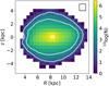 |
Fig. 1. Star counts from our high-quality Gaia DR2 6D sample in bins of width 1.0 kpc in R and z, as indicated by the box in the upper right corner. The central coordinates of the bins are separated by 0.5 kpc in R and z, thus the bins are not fully independent. The white contours indicate the location of bins with 2000 (inner contour) or 100 (outer contour) stars. The position of the Sun is indicated by the white symbol. Only stars with |

We derive the velocities of the stars in our sample in a Galactocentric cylindrical coordinate system (vR, vz, vϕ). For the motion of the Local Standard of Rest (LSR), that is the velocity of a circular orbit at R = R⊙, we assume vc(R⊙) = 240 km s−1 (Piffl et al. 2014; Reid et al. 2014). The peculiar motion of the Sun with respect to the LSR is taken to be (U, V, W)⊙ = (11.1, 12.24, 7.25) km s−1 (Schönrich et al. 2010), where U denotes motion radially inwards and V in the direction of Galactic rotation (both in the Galactic plane), and W perpendicular to the Galactic plane and in the direction of the Galactic north pole. We propagate the errors and correlations in the observables to determine the errors on the velocities (and their correlations). Here we assume that the Bayesian distances are not correlated with the remaining astrometric parameters. The velocity errors for the stars in our sample at  kpc are typically smaller than 2 km s−1 with a median value of ∼1 km s−1 for the vR-, vz-, and vϕ-components. At
  kpc the median errors are in the range from ∼3 km s−1 to ∼8 km s−1 and generally smaller than 15 km s−1.
The characterisation of the kinematics, in terms of the mean motions and velocity dispersions, of a large part of the Milky Way disk have been presented in Gaia Collaboration (2018c) using the 6D dataset from Gaia DR2. This characterisation has put on firm ground the evidence of the presence of streaming motions in all velocity components (Siebert et al. 2008; Williams et al. 2013; Tian et al. 2017; Carrillo et al. 2018) and revealed a large amount of substructure in the velocity distributions. In this paper we proceed to focus on the correlation between the radial and vertical velocity components across a large fraction of the Milky Way galaxy.
3. Methods
The 3D velocity distribution of stars f(vϕ, vR, vz) at a given point in the Galaxy may be characterised by its various moments. As described in the Introduction, the tilt of the velocity ellipsoid refers to the orientation of the 2D velocity distribution f(vR, vz), which would be obtained by integrating over vϕ. As shown in Smith et al. (2009) and Büdenbender et al. (2015), this is equivalent to taking the moments of the 3D velocity distribution and neglecting the cross terms with vϕ. These cross-terms are interesting in their own right, as they reveal also other physical mechanisms at work, such as for example the presence of substructures associated to resonances induced by the rotating Galactic bar (Dehnen 1998), but are not the focus of this work.
3.1. The tilt angle: the orientation of the velocity ellipse
In the Galactocentric cylindrical coordinate system we define the tilt angle γ, following for instance Smith et al. (2009), as:
 (1)
(1)
which therefore takes values from −45° to +45°, and is measured counterclockwise (i.e. from the vR-axis towards the positive vz-axis). For exact cylindrical alignment γcyl = 0° and the major and minor axis align with the Galactocentric cylindrical coordinates.
It is also possible to define a tilt angle α with respect to the spherical coordinate system (r, θ, ϕ), where tan(θ)≡R/z, that is:
 (2)
(2)
The tilt angle α thus measures directly the deviation from spherical alignment, which corresponds to α = 0°. In such a case one of the principal axes of the ellipse points to the Galactic centre. The relation between α and γ at every (R, z) is
 (3)
(3)
From now on, we always refer to the tilt angle γ, thus as defined in the cylindrical coordinate system, unless stated otherwise. To explore the spatial variation of the tilt angle we measure the intrinsic moments of Eq. (1) after projecting all stars onto the (R, z)-plane, thus ignoring in the first stage the Galactic azimuthal angle of the stars (although this is considered in Sect. 4.2). We bin the meridional plane as in Fig. 1 and always require at least 100 stars per bin.
3.2. Accounting for measurement errors
Measurement errors affect the observed velocity moments and can therefore have a significant effect on the inferred tilt angles (Siebert et al. 2008). To establish their effect we here explore two “methods” to account for the errors and for recovering the (intrinsic) velocity moments.
Method 1. We assume that the stars in a given spatial bin have similar measurement errors. This assumption is reasonable because the measurement errors in a particular bin are usually much smaller than the intrinsic velocity dispersion. If the measurement errors were exactly the same for all stars in a bin, the intrinsic velocity covariance matrix can be recovered by subtracting the error covariance matrix from the observed velocity covariance matrix. This follows from the fact that convolving a Gaussian distribution with Gaussian distributed measurement errors again results in a Gaussian with covariance matrix Σobs = Σintr + Σerror, where Σobs and Σintr are the observed and intrinsic covariance matrix of the velocity distribution respectively. In our approximation Σerror ≈ median(Σerror,i) for
 (4)
(4)
in which the diagonal terms denote the variance error of the corresponding velocity component of star i. Similarly cov(vR, i, vz, i) denotes the error covariance for the (vR, vz) measurements of star i. For the required typical errors we take the relevant median errors of the stars in the bin. The recovered intrinsic velocity moments are then used to characterise the velocity distribution. The errors on these moments are analytically estimated and then propagated into uncertainties on the recovered tilt angles. More details can be found in Appendix A.
Method 2. We perform Markov chain Monte Carlo (MCMC) modelling (Foreman-Mackey et al. 2013) for bins with a smaller number of stars (with 100 < N < 2000). This aims to solve for the intrinsic velocity dispersions σ(vR)intr and σ(vz)intr, the mean velocities ⟨vR⟩ and ⟨vz⟩, and the covariance term cov(vR, vz)intr in each bin. This is done by maximizing the bivariate Gaussian likelihood function  , where
![Mathematical equation: $$ \begin{aligned} L_i&= L_i[\langle { v}_R \rangle , \sigma ({ v}_R)_{\rm intr}, \langle { v}_z \rangle , \sigma ({ v}_z)_{\rm intr}, \mathrm{cov}({ v}_R, { v}_z)_{\rm intr}] \nonumber \\&= \frac{1}{\sqrt{\mathrm{det}(2 \pi \boldsymbol{\Sigma _i})}} \exp \left[ -\frac{1}{2} (\boldsymbol{x_i} -\boldsymbol{\mu })^\intercal \boldsymbol{\Sigma _i}^{-1} (\boldsymbol{x_i}-\boldsymbol{\mu }) \right] , \end{aligned} $$](/articles/aa/full_html/2019/09/aa35264-19/aa35264-19-eq14.gif) (5)
(5)
in which xi = [vR, i, vz, i], μ = [⟨vR⟩,⟨vz⟩] and Σi = Σintr + Σerror,i. Whereas in Method 1 Σerror,i was assumed to be the same for each star, we here use Σerror,i for each star separately. We add priors to the model that only allow for positive velocity dispersions in vR and vz and that restrict the correlation coefficient between vR and vz always to be within [−1,1]. For a given bin, the samples drawn by the MCMC run translate into a distribution of tilt angles. We take the median as the best estimate of the tilt angle. For its error we take half the difference between the tilt angles corresponding to the 16th and 84th percentile.
In general we find that the effect of the measurement errors on the recovered moments is small. Moreover, for most bins the velocity measurement errors are sufficiently similar and small that we may use the computationally much faster Method 1 instead of the MCMC-based deconvolution. We have also compared the results to the case in which we simply compute the variances of the observed stellar velocities in the bins of interest, and take these at face value, meaning that we do not take into account the measurement errors. The results are again rather similar, see for example, Fig. A.1 which shows the distributions of the measurement errors for the bin located at R = 11.5 kpc and z = 1.5 kpc. In what follows, we use the results from Method 1 unless stated otherwise.
4. Results
We present our measurement of the tilt angles by showing velocity ellipses in the meridional plane. At each position (R, z), we define a set of axes with vR into the R-direction and vz in the z-direction. The centre of each velocity ellipse is always placed at its position (R, z). The size of the major and minor axis of each ellipse scale with the intrinsic velocity dispersions along these directions. The R- and z-axis are both scaled by the same constant cx. Similarly, all vR- and vz-axes are scaled by a constant cv, thus both sets of axes have an aspect ratio of 1. As a consequence, the velocity ellipses drawn will actually point to the Galactic centre when there is spherical alignment. As a reference, the inset in the figures shows a velocity distribution aligned in cylindrical coordinates and with σ(vR)=100 km s−1 and σ(vz) = 50 km s−1 (unless stated otherwise).
4.1. Tilt angles projected onto the (R, z)-plane
Figure 2 shows the velocity ellipses colour-coded by their angular misalignment with respect to spherical alignment. For z ≥ 0 kpc we define this misalignment as γ − γsph, whereas for z < 0 kpc the misalignment is γsph − γ. Steeper tilt angles result in positive misalignment (from light to dark red), shallower tilt angles in negative misalignment (from light to dark blue). Ellipses that are consistent with spherical alignment are greyish. At the midplane it is however not possible to distinguish between spherical and cylindrical alignment, since both γsph = γcyl = 0° at z = 0 kpc, thus here consistency with spherical alignment also implies consistency with cylindrical alignment. Only away from the midplane it is possible to differentiate between these types of alignment.
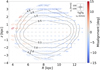 |
Fig. 2. Velocity ellipses in the meridional plane. The ellipses are colour-coded by their misalignment with respect to spherical alignment. The orientation that corresponds to spherical alignment is indicated by the dotted grey line through each ellipse. The inset in the top right of the figure shows the velocity ellipse for a non-tilted distribution with dispersions σ(vR)=100 km s−1 and σ(vz)=50 km s−1 (see Sect. 4 for more information). The contours show the (relatively small) formal statistical errors on the recovered tilt angles and are drawn for error levels of [0.5, 1.0, 2.0, 4.0] degrees. See Sect. 5 for a discussion on the effect of systematic errors. |
We further add contours of constant formal statistical error values on the recovered tilt angles in Fig. 2. We have drawn contours for errors reaching 0.5, 1.0, 2.0, and 4.0 degrees. These contours show the great quality of our dataset over the distance range explored.
From this figure it is evident that there are just a few bins that have tilt angles much steeper than spherical alignment (i.e. there are just two dark red ellipses). These are however located in the inner regions of the Galaxy and at those positions where the error on the tilt angle is also large.
In general, however, the following trend is apparent: for Galactocentric spherical radius r ∼ 4 kpc, the orientations of the velocity ellipses seem to be slightly steeper than spherical alignment. For r ∼ 7 kpc they seem fully consistent with spherical alignment. For larger radii, that is R > 8 kpc and |z|≳1 kpc, the ellipses have a negative misalignment, meaning that the orientations of the ellipses become shallower compared to prediction for spherical alignment. Here the orientation thus changes into the direction of cylindrical alignment and is no longer consistent with spherical alignment.
To be able to assess whether the tilt angles found are more consistent with spherical or cylindrical alignment we show them with error bars in Fig. 3 as a function of height for four Galactic radii, namely R = [5, 7, 9, 11] kpc. The red squares (without error bars; labelled “Raw data”) follow from computing the moments directly from the data, and the green diamonds (“Analytic”) and blue crosses (“MCMC”) are derived using Method 1 and Method 2 respectively, thus accounting for the measurement errors (see Sect. 3.2). They give consistent results given the error bars, although the MCMC-method seems to result in slightly steeper tilt angles.
 |
Fig. 3. Tilt angles as a function of Galactic height for different positions across the Galaxy. We show the trends with z for R = [5, 7, 9, 11] kpc. The red squares, green diamonds, and blue crosses are based on the methods described in Sect. 3.2 (see text). The solid black line shows the trend that would correspond to spherical alignment. The tilt angle is changing from spherical alignment in the inner Galaxy (R ∼ 5 kpc) towards shallower tilt angles at R ∼ 11 kpc. The cyan line shows the analytic description of the data as proposed in Sect. 4.4. |
The black curve in Fig. 3 shows the expectation in the case of spherical alignment. At R = 5 kpc (left panel) the recovered tilt angles are in agreement with spherical alignment for the heights explored. At R = 7 kpc (left centre panel) the data is consistent with spherical alignment up to |z|∼2 kpc. For larger heights the tilt angles are only mildly shallower. For R = 9 kpc and R = 11 kpc, however, the tilt angles are becoming increasingly shallower with respect to spherical alignment. In fact, for R = 12 kpc (see Fig. 2) the orientation of the ellipses become more consistent with cylindrical alignment for the heights probed.
4.2. Tilt angles for different azimuthal angles
Since the Galaxy is not axisymmetric we now investigate whether the tilt angles vary with azimuth by taking into account the 3D location of the individual stars in our dataset. We bin the data into Cartesian bins (x, y, z) whose volume is fixed to 1 × 1 × 1 kpc3, which implies that the different azimuthal cones we explore contain independent data for R > 4 kpc. These cones are centred on three different angles ϕ = [165 ° ,180 ° ,195 ° ].
The resulting maps are shown in Fig. 4. Since the data is effectively sliced in ϕ, the number of stars at a given (R, z) is lower and as a consequence the spatial bins cover a smaller spatial extent in comparison to Sect. 4.1. A coarse comparison of the different panels in this figure suggests that the variations with azimuth are relatively small compared to the global trend that is still apparent in each panel: the misalignment changes from positive to negative when moving outwards in Galactic radius.
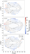 |
Fig. 4. Velocity ellipses in the meridional plane, now for different positions in azimuth (ϕ = [165 ° ,180 ° ,195 ° ] from top to bottom, respectively). The spatial bins are cubes in (x, y, z), of 1 kpc on a side. The colours of the ellipses represent the misalignment with respect to spherical alignment (as in Fig. 2). |
The most prominent differences are seen for the bins at R ∼ 4 kpc and z ∼ 1 kpc. The ϕ = 180°-slice indicates much steeper tilt angles than the ϕ = 195°-slice. The statistical errors on these tilt angles are however large. In fact, most of these bins have consistent tilt angles given their error bars.
For a more direct comparison we show in Fig. 5, for specific radii R = [6, 8, 10] kpc, the tilt angles for the different Galactic azimuths as a function of Galactic height. Here the different symbols, namely red squares, green diamonds, and blue crosses correspond to the measurements for ϕ = [165 ° ,180 ° ,195 ° ], respectively. The black starred symbols show the measurements from all stars at the given R and z and irrespective of azimuth (as in Sect. 4.1). At R = 10 kpc the tilt angles for the different azimuths are less consistent with spherical alignment than those at R = 6 kpc, especially at positive Galactic heights.
 |
Fig. 5. Tilt angles as a function of Galactic height for different radial and azimuthal positions across the Galaxy. The red squares, green diamonds, and blue crosses show the measurements for ϕ = [165 ° ,180 ° ,195 ° ], respectively. The black starred symbols show the measurements irrespective of azimuth (as in Sect. 4.1). Given the error bars, there are only small differences in the tilt angles for the different azimuths explored. The solid black line denotes the trend expected for spherical alignment. |
Even though some bins reveal slight differences in the tilt angles when varying Galactic azimuth, the overall qualitative trends are similar to the case in which we projected all stars onto the (R, z)-plane, thus justifying the approach used in Sect. 4.1. These results also suggest that the degree of non-axisymmetry, in terms of the tilt angles, is modest over the azimuthal range explored.
4.3. Variations with stellar populations
In this section we explore whether different populations of stars follow similar trends in tilt angle. To this end we have cross matched the full Gaia DR2 catalogue with three spectroscopic datasets: the Large Sky Area Multi-Object Fiber Spectroscopic Telescope (LAMOST DR4; Cui et al. 2012), RAVE DR5, and APOGEE DR14. If a star has radial velocity measurements from more than one survey, we take the measurement with the smallest quoted error. As for the spectroscopic sample delivered as part of Gaia DR2 (Arenou et al. 2018), we only consider stars whose radial velocity errors have been estimated to be smaller than 20 km s−1. By adding radial velocities from these other surveys the number of stars with full phase-space information is increased by over 30%.
To explore dependences on populations, we only use metallicities from LAMOST DR4 since this survey probes a much larger region than either RAVE or APOGEE. We refrain from merging the metallicity information from the different surveys to avoid possible offsets between metallicity scales. Finally, only stars with metallicity uncertainties up to 0.2 dex are considered in our analysis.
A downside of extending our sample is that Bayesian distances are missing for the newly added stars to our sample. Since the purpose of this section is to inspect variations between different populations, we here approximate the distances to the stars by  , where
 (6)
(6)
For the following analysis, we select those stars with at most 20% relative distance errors, that is  , and
, and  kpc. We proceed to classify the stars according to a halo population as those with [M/H] < −1.0 dex, a thick disk population for −1.0 < [M/H] < −0.5 dex, and a thin disk population for [M/H] > −0.4 dex. With these criteria, our sample contains ∼23 000 halo stars, ∼260 000 thick disk stars, and ∼2 million thin disk stars.
Figure 6 shows the velocity ellipsoids and tilt angles as a function of position in the meridional plane for the halo (left), thick disk (middle), and thin disk (right) subsamples. The different spatial coverage of the subsets reflect differences in the number of stars (recall that to reliably measure a tilt angle we require at least 100 stars in a spatial bin). In addition the ellipses for the halo population are much larger compared to those of the thick and thin disks. In fact, we have had to use different scales for the panels: the insets in the bottom right of each panel show ellipses whose semi-major and semi-minor axes correspond to dispersions of σ(vR)=200 km s−1 and σ(vz)=100 km s−1 for the halo and thick disk populations, and to σ(vR)=100 km s−1 and σ(vz)=50 km s−1 for the thin disk.
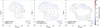 |
Fig. 6. Velocity ellipses in the meridional plane, as in Fig. 2, but now for the subsamples representing halo (left), thick disk (middle) and thin disk (right) populations. We note that the scaling of the velocity ellipses, indicated by the insets in the bottom right of each panel, are different. The colour coding of the ellipses represents the misalignment with respect to spherical alignment and is the same as in Fig. 2. There is no strong evidence that the tilt angles of the different populations behave differently. |
As in previous sections, the colours in Fig. 6 represent the misalignment of the tilt angles with respect to spherical alignment. The same trends as found earlier are visible for the populations independently: at R ≲ 7 kpc the alignment is closer to spherical, while outwards from R ∼ 9 kpc the misalignment becomes negative, which means that the tilt angles become shallower. This can be seen more easily when comparing the tilt angles derived for each population at specific radii, as shown in Fig. 7.
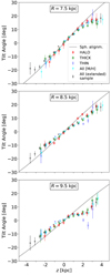 |
Fig. 7. Tilt angles as a function of Galactic height for different populations of stars. We show the trends with z for R = 7.5 kpc (top), R = 8.5 kpc (middle) and R = 9.5 kpc (bottom). The red squares, green diamonds, and blue crosses show the results for the halo, thick, and thin disk population described in Sect. 4.3, respectively. The light blue triangles correspond to all LAMOST stars with metallicity information with uncertainties smaller than 0.2 dex, while the black stars are for all stars in the extended sample regardless of whether or not they have metallicity information. The solid black line shows the trend that would correspond to spherical alignment. |
There are also some differences seen. For example, at R = 8.5 kpc, the halo sample seems to be more consistent with spherical alignment than both disk samples. For R = 9.5 kpc, however, the differences between the populations are minor, except for the flatter thin disk tilt angles at z ∼ 2.5 kpc. Therefore we may conclude that the results shown in Sect. 4.1 are not strongly dependent on the different populations present throughout the volume probed by our dataset.
4.4. Quantifying the degree of spherical alignment
Because the trends seen in the tilt angles are not strongly dependent on Galactic azimuth nor on stellar population, we here aim to provide a simple description of their variation with radius R and height z as found in Sect. 4.1. Since we infer near spherical alignment for R ∼ 6 kpc, we consider expanding α around a point (R0, z0):
 (7)
(7)
where ai are constants and both R and z in kpc2. By definition α(R0, z0) = 0°. We further set z0 = 0 kpc (i.e. the symmetry plane of α is set to be the Galactic midplane). Moreover, a1 = a4 = 0, since for most realistic models the tilt angle does not vary at the midplane. By symmetry arguments the coefficients of all even powers of z (including a5) must be zero, since α is expected to be either antisymmetric with respect to the midplane or zero. Since we have found that at R ∼ 6 kpc the tilt angles are consistent with spherical alignment for all z probed (see left panels of Fig. 3), we additionally set a2 = 0 such that at R = R0: α(R0, z) = 0°. With these choices:
 (8)
(8)
We thus fit this functional form to the data to derive values for R0 and a3 such that the χ2-statistic defined as:
![Mathematical equation: $$ \begin{aligned} \chi ^2 = \sum _{j=1}^{N_\mathrm{bins} } \left( \frac{\alpha (R_j, z_j)_\mathrm{model} - \alpha (R_j, z_j)_\mathrm{obs} }{\epsilon [\alpha (R_j, z_j)_\mathrm{obs} ]} \right)^2 . \end{aligned} $$](/articles/aa/full_html/2019/09/aa35264-19/aa35264-19-eq21.gif) (9)
(9)
is minimised. Here j runs over the number of bins Nbins where a measurement is made, in other words where N > 100 stars.
For most bins at |z| ≤ 2.0 kpc and 5 ≤ R ≤ 12 kpc the inferred statistical errors on the tilt angles are very small (e.g. see the dashed contours in Fig. 2). In that case systematic errors need to be considered. One such source of systematic errors are substructures. We performed tests to estimate the effect of substructures in velocity space on the tilt angle. To this end we inserted Nsub = 1, 4, 9, 16, 25, or 36 substructures on smooth non-tilted velocity distributions with velocity dispersions of 20 km s−1 and 35 km s−1 in vz and vR (i.e. values representative of the thin disk near R ∼ R⊙), respectively. Each substructure was assigned a random number of stars such that the total fraction of stars in substructures is fsub = 5%, 10%, 15%, or 20%. We randomly assigned velocity dispersions to the substructures, drawn uniformly from 1 km s−1 to 5 km s−1 in both directions. For each combination of (Nsub, fsub) we considered 100 realisations. The median (absolute) tilt angle found from these experiments is ∼1°, implying that this value is representative of the error introduced by neglecting the presence of substructures in a velocity distribution. This result is independent of the total number of stars N for N ≳ 10 000 (a value that is representative of the number of stars in the bins with ϵ[α(Rj, zj)] < 1°). Thus, when minimising the χ2 we consider a floor for the statistical error ϵ[α(Rj, zj)] in each bin of 1°.
We fit to find R0 = (6.16 ± 0.16) kpc and a3 = (0.72 ± 0.04)°/kpc2 resulting in a reduced χ2 of 1.65. The cyan line in Fig. 3 shows the tilt angles predicted by this fit, which reproduces relatively well the trends observed in the data. The model goes through the 1σ-error bars for approximately 60% of all spatial bins, while for 98% of bins the model matches the data within 3× the estimated uncertainty. This indicates that our simple model provides a fair description of the behaviour of the tilt of the velocity ellipsoid across the Galactic volume probed by our dataset.
The fact that the total reduced χ2-value is greater than unity indicates that the tilt angles for some bins are not fitted very well by the model. For example at R ∼ 10 kpc the tilt angles as inferred from the data are asymmetric with respect to the z = 0 plane: at z > 0 kpc they more or less attain a constant value of ∼2.0°, whereas below the midplane the tilt angles become steeper with z (e.g. −15° at z = −3.0 kpc). The fits at such radii are therefore relatively poor. For the bins between R = 11 kpc and R = 12 kpc, we notice that the observed tilt angles seem to have a small positive offset from zero near z = 0. These offsets are small (of order 2°), although they do affect the goodness of fit measure.
5. Discussion
5.1. The impact of (parallax) measurement errors on the recovered tilt angles.
Gaia Collaboration (2018a) have reported the presence of a systematic error on the Gaia DR2 parallaxes in the form of a zero-point offset of a few 10 of μas (in the sense that Gaia parallaxes are too small) and whose exact amplitude depends on location on the sky. Such systematic zero-point offset affects the tangential velocities of the stars, which are determined from both distances and proper motions. The overall systematic parallax offset in Gaia DR2 was determined using distant quasars by Lindegren et al. (2018) to be approximately −29 μas, with a large rms of ∼43 μas. Arenou et al. (2018) using different samples of objects (RR Lyrae stars, Magellanic Clouds, open clusters, dwarf spheroidal galaxies, etc.) report important variations in the zero-point offsets, highlighting the complexity of the offset. Nonetheless all values are consistent given the large estimated rms.
Around the time this paper was submitted, Schönrich et al. (2019) reported a new estimate of the parallax zero-point offset based on the distance estimation method used in Schönrich & Aumer (2017) (also see Schönrich et al. 2012). These authors argue for a much larger zero-point for the parallaxes in the RVS subset of Gaia DR2, namely of magnitude −54 ± 6 μas. Zinn et al. (2019) and Khan et al. (2019) applied asteroseismology to determine distances to Red Giant Branch (RGB) and Red Clump (RC) stars with GaiaG-band magnitudes similar to those present in the RVS subset of Gaia DR2 and determined an offset close to −50 μas, while Sahlholdt & Silva Aguirre (2018), using asteroseismology information on dwarfs, report that the offset could be ∼ − 35 ± 16 μas. More recently Hall et al. (2019), using RC stars with asteroseismology, estimate the mean offset to be −41 ± 10 μas. These comparisons suggest that the offset could well be larger for the brighter stars of the Gaia RVS sample but that its amplitude is quite uncertain.
5.1.1. Quantification of the impact of a zero-point offset
We first quantify how the tilt angles are affected if parallaxes are underestimated. For illustration purposes, we estimate the impact on the recovered tilt angles induced by a systematic error (with mean −29 μas) while also including the effects of random errors3. Their effect is examined by using the Gaia Universe Model Snapshot (GUMS; Robin et al. 2012), which is based on the Besançon Galaxy Model (Robin et al. 2003).
We mimic the Gaia DR2 subsample with full phase-space information, by selecting stars in GUMS that have G < 13 mag, as this is roughly the magnitude limit for radial velocities in Gaia’s current data release. We generate 100 data realisations by convolving the (error-free) GUMS sample with a Gaussian with Gaia DR2-like random and systematic errors for the parallaxes (Lindegren et al. 2018). The systematic parallax offsets for the stars are drawn from a Gaussian with mean −29 μas and standard deviation of 30 μas4. To obtain a distance estimate we invert the parallaxes and consider only those stars that satisfy ϖ/ϵ(ϖ) > 5 and ϖ ≳ 200 μas. Here ϖ is the observed parallax and ϵ(ϖ) the random parallax error and thus the same quality criteria are applied as to the real data (see Sect. 2).
For each spatial bin the median (over all realisations) of the distribution of tilt angles is compared to the tilt angles from the error-free model, on the meridional plane. The error-free GUMS model has close to cylindrically aligned velocity ellipses (γGUMS ∼ 0°). The impact of the random and systematic parallax uncertainties on the tilt angles depends on location as can be seen in the left panel of Fig. 8. At R ≲ 7 kpc the orientations of the velocity ellipses change towards the direction of spherical alignment (ΔγGUMS > 0 for z > 0 and ΔγGUMS < 0 for z < 0), while for R ≳ 9 kpc the change is in the opposite sense.
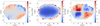 |
Fig. 8. Left: differences in tilt angles, ΔγGUMS, between error convolved realisations (taking into account random and systematic parallax errors) and the error-free GUMS catalogue. Centre: standard deviation of the tilt angles over all realisations. Right: division of the differences by the corresponding standard deviation. At distances at around 2 kpc the changes are significant with respect to the scatter present between realisations. |
The middle panel of Fig. 8 shows the spread in tilt angles over all realisations, and reveals that the errors result in a spread with a typical amplitude of ≲4°, except for the outermost bins, where it can be twice as large, and hence comparable to ΔγGUMS. The right panel shows at which locations the median change in tilt angles, caused by parallax errors, is larger than the rms from realisation to realisation. For bins located at distances of ∼2 kpc a change in tilt angle due to parallax errors is thus likely to occur in a preferential direction, with the amplitude of this change varying from realisation to realisation.
These findings imply that, if parallaxes are underestimated, the tilt angles inferred may appear steeper than they really are in the inner Galaxy, while the opposite happens in the outer Galaxy, thus the tilt angles become shallower there. If we take the results from GUMS at face value, |ΔγGUMS|≈6° at (R, |z|) ∼ (5, 3) kpc, which means that an unaccounted for zero-point offset of magnitude 29 μas in the parallaxes affects the inferred tilt angles such that they appear steeper by ∼6°. This does not radically change the type of alignment at this location (where spherical alignment would imply γ ∼ 30°). For (R, |z|) ∼ (11, 2) kpc we find that |ΔγGUMS| can attain values close to 5°, which is of similar amplitude as the misalignment seen in Fig. 2. Although the GUMS tilt angles intrinsically have γGUMS ∼ 0°, we find similar amplitudes for the cases explored in Appendix B, where we start from both intrinsically spherically and cylindrically aligned ellipsoids.
In the analysis presented in previous sections, we have effectively corrected for the parallax offset by using the McMillan (2018) distances. If the assumed parallax zero-point is too small, the results presented in this section indicate that, especially towards the outer Galaxy, the zero-point offset could produce tilts that are less steep than what they are intrinsically. We explore such a larger offset next.
5.1.2. A zero-point offset as large as −54 μas
Everall et al. (2019) have derived tilt angles using the Schönrich et al. (2019) Bayesian distance estimates (with parallax zero-point of −54 μas). These authors showed that the tilt angles appear to be much more consistent with spherical alignment when using those distances.
Since the method used in Schönrich et al. (2019) assumes spherical alignment, we preferred not to directly use their distances while testing for the effect of a large −54 μas offset. Therefore we here also explore how the tilt angles change if the parallax offset would be as large as −54 μas, by comparing them to the case in which the offset is −29 μas. For both cases we take the extended sample and invert the parallaxes after correcting for the zero-point offset (as in Sect. 4.3), such that the changes due to the differences in parallax offset can be easily compared.
In Fig. 9 we show the results. The blue squares have been calculated after correcting for a parallax zero-point offset of −29 μas, whereas for the orange diamonds a value of −54 μas is assumed. For the outer Galaxy (R = 9 kpc and R = 11 kpc) such a larger parallax zero-point can modify the tilt angles such that they are more consistent with spherical alignment, in agreement with our analysis of the previous section.
 |
Fig. 9. Tilt angles as a function of Galactic height for different positions across the Galaxy. We show the trends with z for R = [5, 7, 9, 11] kpc for different distance estimates for the stars. The blue squares and orange diamonds use distances based on inverting the parallaxes after correcting the parallaxes for an offset of −29 μas and −54 μas, respectively. The green crosses and red starred symbols use Bayesian distances from McMillan (2018) and Schönrich et al. (2019), respectively. The solid black line shows the trend that would correspond to spherical alignment. |
A direct comparison of the tilt angles obtained using McMillan (2018) Bayesian distances (who assumes a zero-point of −29 μas, green crosses) with the results obtained from inverting the parallaxes after correcting for a zero-point of −29 μas (blue squares), shows good agreement except for R = 5 kpc. At this location, it would seem as if the choice of the distance estimator would play a role in the determination of the tilt angle. The Bayesian distances result in tilt angles that are just slightly steeper than expected for spherical alignment, while inverting the parallaxes results in much shallower tilt angles (the larger the offset assumed the shallower the tilt angles). On the other hand, comparing the tilt angles obtained using Schönrich et al. (2019) Bayesian distances (who find a zero-point of −54 μas, red starred symbols), with the results obtained from inverting the parallaxes after correcting for a zero-point of −54 μas (orange diamonds), shows rather similar trends at R = 5 kpc. At the other radii shown, these Bayesian distances also result in tilt angles that are in good agreement with inverting the parallaxes.
The analysis presented in the last two sections shows that the amplitude of the systematic error in the parallax, in the form of a zero-point offset, plays a role in the determination of the tilt angles for the outer Galaxy (R > 9 kpc). Since the offset is known to vary with celestial position, magnitude and colour, it is difficult at this point to properly correct for it, and this impairs a very accurate determination of the tilt angle throughout the range of distances probed. However, recall that the range of zero-point offsets is bracketed by the values explored (i.e. from −54 μas to −29 μas), so the analysis presented here gives us a handle on the possible outcomes.
5.2. Constraints to models of the Milky Way
Several models of the Milky Way have been proposed by matching a variety of constraints (e.g. McMillan 2011, 2017; Piffl et al. 2014). Particularly useful for the interpretation of the findings reported in this paper are Stäckel models (e.g. de Zeeuw 1985; Dejonghe & de Zeeuw 1988). Axisymmetric models with a potential of Stäckel form have the property that the equations of motion are separable in their spheroidal coordinates. Therefore the principal axes of the velocity ellipsoids are always aligned with these coordinates (also see: Eddington 1915). The foci of such a coordinate system then determine the alignment at each position. For a composite model to be of a Stäckel form, the locations of the foci must be identical for all components.
Famaey & Dejonghe (2003), for example, have extended the two-Stäckel component work of Batsleer & Dejonghe (1994) by adding a third component, such that the model could allow for a thin and thick disk, in addition to a halo component. The authors use constraints such as the (flat) rotation curve, circular velocity at the position of the Sun, the Oort constants, and the local total mass density in the disk to search for a set of consistent parameters for their Stäckel models. Here we take the set of prolate spheroidal coordinates, (λ, ϕ, ν), from Famaey & Dejonghe (2003, mass model II). The foci of this oblate mass model are located at (R, z) = (0, ±0.88) kpc. At R ∼ 0 and |z|≲0.88 kpc such spheroidal coordinates align with the cylindrical coordinate system (see Fig. 10). Outside of these foci and with increasing distance from the Galactic centre the spheroidal coordinates approach the spherical coordinate system. In general, any (composite) Stäckel model predicts a change in the tilt of the velocity ellipse from cylindrical to spherical alignment. The transition radius depends on the location of the foci.
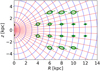 |
Fig. 10. Contours of constant prolate spheroidal coordinates, (λ, ν), with foci at R = 0 and z = ±0.88 kpc (see text). Contours of constant λ are shown in blue, contours of constant ν in red. The green ellipses show some of our measured velocity ellipses (Method 1). Their orientation does not align with the coordinate contours at R ≳ 10 kpc and |z|≳2 kpc. |
Since the observed tilt angles at R ∼ 4 kpc already show near spherical alignment, this implies foci at |z|≲4 kpc. Their exact position would depend on whether the innermost region of the Galaxy, not probed by our dataset, is cylindrically aligned or not, and if so at what distance the transition occurs. However, the tilt angles in the outer Galaxy (9 ≲ R ≲ 12 kpc) derived using the McMillan (2018) distances are not consistent with Stäckel models that have foci at |z|≲4 kpc, and would require a larger focal distance. We have numerically checked these statements by comparing the predicted tilt angles of both oblate and prolate Stäckel models (for a large range of different focal distances) to the observed tilt angles while taking into account their errors.
There are of course many more models with bulge, disk and halo components, for example spherical bulge, exponential disk, Navarro–Frenk–White (NFW; Navarro et al. 1996) halo, or Miyamoto & Nagai (1975) models. The separable models are in that sense a subset but have the advantage that for them the tilt of the velocity ellipsoid is dictated by the coordinate system in which the equations of motion (Hamilton–Jacobi equation to be more precise) separate.
Piffl et al. (2014) have applied a five component mass model (gas disk, thin and thick disk, flattened bulge and dark halo) to RAVE DR4 stars. Using their best-fitting parameters we computed the relevant velocity moments from the distribution function for a similar range in R and z as probed in our dataset. The tilt angles for this model are spherically aligned for R ≳ 7 kpc and are, as in the separable models discussed above, changing towards cylindrical alignment with decreasing R.
In Fig. 11 we show the tilt angles for both the Stäckel model (purple line) of Famaey & Dejonghe (2003) and the Piffl et al. (2014) model (orange line), for radii R = 6 kpc and R = 10 kpc. The green diamonds indicate the tilt angles as found by Method 1. Since this Stäckel model has focii at |z|≲0.88, which is very close to the Galactic centre with respect to the innermost radius probed in our dataset, the Stäckel model is almost indistinguishable from spherical alignment for all positions probed. The Piffl et al. (2014) model has tilt angles that are shallower at R = 6 kpc, but also approaches spherical alignment with increasing Galactic radius. At R = 10 kpc, for example, the tilt angles from the Piffl et al. (2014) model are seen to nearly coincide with the expectation for spherical alignment.
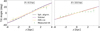 |
Fig. 11. Tilt angles for both the Stäckel (purple line) and Piffl et al. (2014, orange line) model for radii at R = 4 kpc and R = 8 kpc (see text). For comparison we add our measurement as green diamonds (Method 1). |
We note that if the parallax zero-point is larger than assumed here the tilt angles do become more consistent with spherical alignment for large radii (see Sect. 5.1.2). This is in line with predictions for both composite Stäckel models as well as for the Piffl et al. (2014) model. In addition, it would be interesting to know whether the tilt angles become shallower towards the central regions of the Galaxy (at R ≲ 4 kpc). In principal it would then be possible to solve for the focal distance. However, the effects of both the type of distance estimator and the assumed parallax zero-point are too large to make firm statements in this region. Future data releases will for sure enable to probe regions closer to the Galactic centre more robustly.
6. Conclusions
We have studied the trends in the tilt angle of the velocity ellipsoids in the meridional plane for a high-quality sample of more than 5 million stars located across a large portion of the Galaxy, from R ∼ 4 kpc to R ∼ 13 kpc, and reaching a maximum distance from the plane of ∼3.5 kpc.
We find that the tilt angles are somewhat dependent on the offset of the Gaia DR2 parallaxes, and that the effects are particularly important for the outer Galaxy. When using the McMillan (2018) Bayesian distances, derived assuming an offset of −29 μas, we find that the tilt angles are consistent with (near) spherical alignment at R ≲ 7 kpc for all heights probed (|z| ≲ 3 kpc). Beyond R ≳ 9 kpc the tilt angles clearly become more shallower than expected for spherical alignment. These trends remain when the stars are separated into “populations” according to their metallicity (as given by LAMOST DR4). We provide a simple analytic function for the tilt angle in spherical coordinates α(R, z)/[deg] ≈ 0.72(R − 6.16)z, that fits well the trend observed as a function of Galactic radius and height, after projecting the stars onto the (R, z)-plane.
We find that if the amplitude of the zero-point offset in the parallax is underestimated, the angles tend to appear shallower than they intrinsically are in the outer Galaxy (i.e. changing into the direction of cylindrical alignment if the ellipsoid is intrinsically spherically aligned). We quantify the impact on the tilt angles when assuming a parallax zero-point as large as −54 μas, as estimated in Schönrich et al. (2019) (also see Everall et al. 2019). Such a large offset (the upper limit of estimates reported in the literature by other authors) does indeed lead to tilt angles that are more consistent with spherical alignment than obtained when using the McMillan (2018) distances. Therefore it will be particularly important to pin-down, in future Gaia data releases, the amplitude of the parallax zero-point as well as its local variations as these affect our ability to constrain the mass distribution in our Galaxy.
Use of the value of R⊙ = 8178 ± 13stat. ± 22sys. pc, as determined by Gravity Collaboration (2019), does not affect the main conclusions of this paper.
We prefer to quantify the deviation from spherical symmetry directly on the spherical tilt angle α than to use the purely geometric parametrisation by Binney et al. (2014) of the cylindrical tilt angle γ′ = a0arctan(z/R)=a0(π/2 − θ) where θ indicates the spatial location of the bin (see also Eq. (3)). Although a0 = 1 implies spherical alignment and a0 = 0 cylindrical alignment, it is not intuitively clear what the quantitive meaning of other a0 values is.
In Appendix B we analytically compute how the vR- and vZ-velocities (and thus their moments and tilt angles) are affected by the parallax zero-point offset alone.
As estimated in Gaia Collaboration (2018b).
If, hypothetically, both  and ⟨U0W0⟩=0, then tan(2δ1)= ± tan(2b).
Acknowledgments
The authors thank the anonymous referee whose insightful comments helped improving the quality of the manuscript. JH thanks Helmer Koppelman for helping in creating the dataset used in this work (Koppelman et al. 2019). AH acknowledges financial support from a VICI grant from the Netherlands Organisation for Scientific Research, N.W.O. TdZ is grateful to the Kapteyn Astronomical Institute for the hospitality during his Blaauw Professorship. This work has made use of data from the European Space Agency (ESA) mission Gaia (https://www.cosmos.esa.int/gaia), processed by the Gaia Data Processing and Analysis Consortium (DPAC; https://www.cosmos.esa.int/web/gaia/dpac/consortium). Funding for the DPAC has been provided by national institutions, in particular the institutions participating in the Gaia Multilateral Agreement. We have also made use of data from: (1) the APOGEE survey, which is part of Sloan Digital Sky Survey IV. SDSS-IV is managed by the Astrophysical Research Consortium for the Participating Institutions of the SDSS Collaboration (http://www.sdss.org). (2) the RAVE survey (http://www.rave-survey.org), whose funding has been provided by institutions of the RAVE participants and by their national funding agencies. (3) the LAMOST survey (www.lamost.org), funded by the National Development and Reform Commission. LAMOST is operated and managed by the National Astronomical Observatories, Chinese Academy of Sciences. For the analysis, the following software packages have been used: vaex (Breddels & Veljanoski 2018), NumPy (Oliphant 2015), matplotlib (Hunter 2007), Jupyter Notebook (Kluyver et al. 2016), TOPCAT and STILTS (Taylor 2005, 2006).
References
- Abazajian, K. N., Adelman-McCarthy, J. K., Agüeros, M. A., et al. 2009, ApJS, 182, 543 [NASA ADS] [CrossRef] [Google Scholar]
- An, J., & Evans, N. W. 2016, ApJ, 816, 35 [NASA ADS] [CrossRef] [Google Scholar]
- Antoja, T., Figueras, F., Fernández, D., & Torra, J. 2008, A&A, 490, 135 [NASA ADS] [CrossRef] [EDP Sciences] [Google Scholar]
- Antoja, T., Helmi, A., Romero-Gómez, M., et al. 2018, Nature, 561, 360 [NASA ADS] [CrossRef] [Google Scholar]
- Arenou, F., Luri, X., Babusiaux, C., et al. 2018, A&A, 616, A17 [Google Scholar]
- Batsleer, P., & Dejonghe, H. 1994, A&A, 287, 43 [NASA ADS] [Google Scholar]
- Belokurov, V., Erkal, D., Evans, N. W., Koposov, S. E., & Deason, A. J. 2018, MNRAS, 478, 611 [NASA ADS] [CrossRef] [Google Scholar]
- Binney, J., & McMillan, P. 2011, MNRAS, 413, 1889 [NASA ADS] [CrossRef] [Google Scholar]
- Binney, J., & Tremaine, S. 2008, Galactic Dynamics, 2nd edn. (Princeton: Princeton University Press) [Google Scholar]
- Binney, J., Gerhard, O., & Spergel, D. 1997, MNRAS, 288, 365 [NASA ADS] [CrossRef] [Google Scholar]
- Binney, J., Burnett, B., Kordopatis, G., et al. 2014, MNRAS, 439, 1231 [NASA ADS] [CrossRef] [Google Scholar]
- Bonaca, A., Hogg, D. W., Price-Whelan, A. M., & Conroy, C. 2019, ApJ, 880, 38 [NASA ADS] [CrossRef] [Google Scholar]
- Bond, N. A., Ivezić, Ž., Sesar, B., et al. 2010, ApJ, 716, 1 [NASA ADS] [CrossRef] [Google Scholar]
- Bovy, J. 2011, PhD Thesis, New York University, USA [Google Scholar]
- Breddels, M. A., & Veljanoski, J. 2018, A&A, 618, A13 [NASA ADS] [CrossRef] [EDP Sciences] [Google Scholar]
- Büdenbender, A., van de Ven, G., & Watkins, L. L. 2015, MNRAS, 452, 956 [NASA ADS] [CrossRef] [Google Scholar]
- Carrillo, I., Minchev, I., Kordopatis, G., et al. 2018, MNRAS, 475, 2679 [NASA ADS] [CrossRef] [Google Scholar]
- Casetti-Dinescu, D. I., Girard, T. M., Korchagin, V. I., & van Altena, W. F. 2011, ApJ, 728, 7 [NASA ADS] [CrossRef] [Google Scholar]
- Cui, X.-Q., Zhao, Y.-H., Chu, Y.-Q., et al. 2012, Res. Astron. Astrophys., 12, 1197 [NASA ADS] [CrossRef] [Google Scholar]
- Dehnen, W. 1998, AJ, 115, 2384 [NASA ADS] [CrossRef] [Google Scholar]
- Dejonghe, H., & de Zeeuw, T. 1988, ApJ, 333, 90 [NASA ADS] [CrossRef] [Google Scholar]
- de Zeeuw, T. 1985, MNRAS, 216, 273 [NASA ADS] [CrossRef] [Google Scholar]
- Eddington, A. S. 1915, MNRAS, 76, 37 [NASA ADS] [CrossRef] [Google Scholar]
- Eggen, O. J. 1965, in Moving Groups of Stars, eds. A. Blaauw, & M. Schmidt (Chicago: University of Chicago Press), 111 [Google Scholar]
- Evans, N. W., Sanders, J. L., Williams, A. A., et al. 2016, MNRAS, 456, 4506 [NASA ADS] [CrossRef] [Google Scholar]
- Everall, A., Evans, N. W., Belokurov, V., & Schönrich, R., 2019, MNRAS, 489, 910 [NASA ADS] [CrossRef] [Google Scholar]
- Famaey, B., & Dejonghe, H. 2003, MNRAS, 340, 752 [NASA ADS] [CrossRef] [Google Scholar]
- Foreman-Mackey, D., Hogg, D. W., Lang, D., & Goodman, J. 2013, PASP, 125, 306 [CrossRef] [Google Scholar]
- Gaia Collaboration (Brown, A. G. A., et al.) 2016, A&A, 595, A2 [NASA ADS] [CrossRef] [EDP Sciences] [Google Scholar]
- Gaia Collaboration (Brown, A. G. A., et al.) 2018a, A&A, 616, A1 [NASA ADS] [CrossRef] [EDP Sciences] [Google Scholar]
- Gaia Collaboration (Helmi, A., et al.) 2018b, A&A, 616, A12 [NASA ADS] [CrossRef] [EDP Sciences] [Google Scholar]
- Gaia Collaboration (Katz, D., et al.) 2018c, A&A, 616, A11 [NASA ADS] [CrossRef] [EDP Sciences] [Google Scholar]
- Gravity Collaboration (Abuter, R., et al.) 2019, A&A, 625, L10 [NASA ADS] [CrossRef] [EDP Sciences] [Google Scholar]
- Hall, O. J., Davies, G. R., Elsworth, Y. P., et al. 2019, MNRAS, 486, 3569 [NASA ADS] [CrossRef] [Google Scholar]
- Helmi, A., Babusiaux, C., Koppelman, H. H., et al. 2018, Nature, 563, 85 [NASA ADS] [CrossRef] [Google Scholar]
- Hunter, J. D. 2007, Comput. Sci. Eng., 9, 90 [NASA ADS] [CrossRef] [Google Scholar]
- Johnson, D. R. H., & Soderblom, D. R. 1987, AJ, 93, 864 [NASA ADS] [CrossRef] [Google Scholar]
- Khan, S., Miglio, A., Mosser, B., et al. 2019, A&A, 628, A35 [NASA ADS] [CrossRef] [EDP Sciences] [Google Scholar]
- King, III, C., Brown, W. R., Geller, M. J., & Kenyon, S. J. 2015, ApJ, 813, 89 [Google Scholar]
- Kluyver, T., Ragan-Kelley, B., Pérez, F., et al. 2016, in Positioning and Powerin Academic Publishing: Players, Agents and Agendas, eds. F. Loizides, & B. Scmidt (IOS Press), 87 [Google Scholar]
- Koppelman, H. H., Helmi, A., Massari, D., Roelenga, S., & Bastian, U. 2019, A&A, 625, A5 [NASA ADS] [CrossRef] [EDP Sciences] [Google Scholar]
- Kunder, A., Kordopatis, G., Steinmetz, M., et al. 2017, AJ, 153, 75 [NASA ADS] [CrossRef] [Google Scholar]
- Lindegren, L., Hernández, J., Bombrun, A., et al. 2018, A&A, 616, A2 [NASA ADS] [CrossRef] [EDP Sciences] [Google Scholar]
- Mackereth, J. T., Bovy, J., Leung, H. W., et al. 2019, MNRAS, accepted [arXiv:1901.04502] [Google Scholar]
- Majewski, S. R., Schiavon, R. P., Frinchaboy, P. M., et al. 2017, AJ, 154, 94 [NASA ADS] [CrossRef] [Google Scholar]
- McMillan, P. J. 2011, MNRAS, 414, 2446 [NASA ADS] [CrossRef] [Google Scholar]
- McMillan, P. J. 2017, MNRAS, 465, 76 [NASA ADS] [CrossRef] [Google Scholar]
- McMillan, P. J. 2018, Res. Notes Am. Astron. Soc., 2, 51 [NASA ADS] [CrossRef] [Google Scholar]
- Miyamoto, M., & Nagai, R. 1975, PASJ, 27, 533 [NASA ADS] [Google Scholar]
- Mood, A. M., Graybill, F. A., & Boes, D. C. 1974, Introduction to the Theory of Statistics, 3rd edn. (New York: McGraw-Hill, Inc) [Google Scholar]
- Navarro, J. F., Frenk, C. S., & White, S. D. M. 1996, ApJ, 462, 563 [NASA ADS] [CrossRef] [Google Scholar]
- Oliphant, T. E. 2015, Guide to NumPy, 2nd edn. (USA: CreateSpace Independent Publishing Platform) [Google Scholar]
- Piffl, T., Binney, J., McMillan, P. J., et al. 2014, MNRAS, 445, 3133 [NASA ADS] [CrossRef] [Google Scholar]
- Poggio, E., Drimmel, R., Lattanzi, M. G., et al. 2018, MNRAS, 481, L21 [NASA ADS] [CrossRef] [Google Scholar]
- Posti, L., Helmi, A., Veljanoski, J., & Breddels, M. A. 2018, A&A, 615, A70 [NASA ADS] [CrossRef] [EDP Sciences] [Google Scholar]
- Price-Whelan, A. M., & Bonaca, A. 2018, ApJ, 863, L20 [CrossRef] [Google Scholar]
- Proctor, R. A. 1869, Proc. R. Soc. London Ser., I, 169 [Google Scholar]
- Rao, C. R. 1973, Linear Statistical Inference and Its Applications, 2nd edn. (New York: John Wiley & Sons, Inc.) [CrossRef] [Google Scholar]
- Reid, M. J., Menten, K. M., Brunthaler, A., et al. 2014, ApJ, 783, 130 [Google Scholar]
- Robin, A. C., Reylé, C., Derrière, S., & Picaud, S. 2003, A&A, 409, 523 [NASA ADS] [CrossRef] [EDP Sciences] [Google Scholar]
- Robin, A. C., Luri, X., Reylé, C., et al. 2012, A&A, 543, A100 [NASA ADS] [CrossRef] [EDP Sciences] [Google Scholar]
- Rose, C., & Smith, M. D. 2002, Mathematical Statistics with Mathematica (Berlin: Springer-Verlag) [Google Scholar]
- Sahlholdt, C. L., & Silva Aguirre, V. 2018, MNRAS, 481, L125 [NASA ADS] [CrossRef] [Google Scholar]
- Schönrich, R. 2012, MNRAS, 427, 274 [NASA ADS] [CrossRef] [Google Scholar]
- Schönrich, R., & Aumer, M. 2017, MNRAS, 472, 3979 [NASA ADS] [CrossRef] [Google Scholar]
- Schönrich, R., Binney, J., & Dehnen, W. 2010, MNRAS, 403, 1829 [NASA ADS] [CrossRef] [Google Scholar]
- Schönrich, R., Binney, J., & Asplund, M. 2012, MNRAS, 420, 1281 [NASA ADS] [CrossRef] [Google Scholar]
- Schönrich, R., McMillan, P., & Eyer, L. 2019, MNRAS, 487, 3568 [NASA ADS] [CrossRef] [Google Scholar]
- Siebert, A., Bienaymé, O., Binney, J., et al. 2008, MNRAS, 391, 793 [NASA ADS] [CrossRef] [Google Scholar]
- Smith, M. C., Wyn Evans, N., & An, J. H. 2009, ApJ, 698, 1110 [NASA ADS] [CrossRef] [Google Scholar]
- Smith, M. C., Whiteoak, S. H., & Evans, N. W. 2012, ApJ, 746, 181 [NASA ADS] [CrossRef] [Google Scholar]
- Stuart, A., & Ord, J. K. 1987, Kendall’s Advanced Theory of Statistics, Volume 1: Distribution Theory, 5th edn. (Glasgow: Charles Griffin & Company Limited) [Google Scholar]
- Taylor, M. B. 2005, in Astronomical Data Analysis Software and Systems XIV, eds. P. Shopbell, M. Britton, & R. Ebert, ASP Conf. Ser., 347, 29 [Google Scholar]
- Taylor, M. B. 2006, in Astronomical Data Analysis Software and Systems XV, eds. C. Gabriel, C. Arviset, D. Ponz, & S. Enrique, ASP Conf. Ser., 351, 666 [Google Scholar]
- Tian, H.-J., Liu, C., Wan, J.-C., et al. 2017, Res. Astron. Astrophys., 17, 114 [Google Scholar]
- van de Ven, G., Hunter, C., Verolme, E. K., & de Zeeuw, P. T. 2003, MNRAS, 342, 1056 [NASA ADS] [CrossRef] [Google Scholar]
- Wegg, C., Gerhard, O., & Bieth, M. 2019, MNRAS, 485, 3296 [NASA ADS] [CrossRef] [Google Scholar]
- Williams, M. E. K., Steinmetz, M., Binney, J., et al. 2013, MNRAS, 436, 101 [NASA ADS] [CrossRef] [Google Scholar]
- Yanny, B., Rockosi, C., Newberg, H. J., et al. 2009, AJ, 137, 4377 [NASA ADS] [CrossRef] [Google Scholar]
- York, D. G., Adelman, J., Anderson, Jr., J. E., et al. 2000, AJ, 120, 1579 [CrossRef] [Google Scholar]
- Zinn, J. C., Pinsonneault, M. H., Huber, D., & Stello, D. 2019, ApJ, 878, 136 [NASA ADS] [CrossRef] [Google Scholar]
Appendix A: Standard errors of sample (co)variances
To estimate the error on the inferred tilt angles from Method 1 of Sect. 3.2 we propagate the errors of the relevant velocity moments from Eq. (1).
The error on a sample variance, s2, can be estimated (e.g. Rao 1973; Mood et al. 1974) by using
 (A.1)
(A.1)
for N stars. Here, μ4 denotes the intrinsic 4th central moment and  , for which vi is the relevant velocity component, either vR or vz, of star i and ⟨v⟩ its mean taken over all stars in the bin considered. The intrinsic velocity moments are estimated by their observed values, which is a good approximation given the relatively small errors in the data for the bins explored.
The error on a sample covariance Sxy of x and y can be estimated (see Stuart & Ord 1987 or Rose & Smith 2002 for using mathStatica) by
![Mathematical equation: $$ \begin{aligned} \mathrm{var} (S_{x{ y}}) = \frac{1}{N} \left[ \mu _{22} - \frac{N-2}{N-1}\mathrm{cov} (x,{ y})^2 + \frac{1}{N-1}\mathrm{var} (x)\mathrm{var} ({ y}) \right] , \end{aligned} $$](/articles/aa/full_html/2019/09/aa35264-19/aa35264-19-eq25.gif) (A.2)
(A.2)
where μ22 = E[{x − E(x)}2{y − E(y)}2] for E denoting the expectation value. We have defined  . In our application x is replaced for vR and y for vz. The intrinsic moments are again estimated by taking the equivalent moments directly from the observed velocity distribution.
As an example for Sect. 3.2 we show in Fig. A.1 the error distributions for the bin at R = 11.5 kpc and z = 1.5 kpc. This bin is near the edge of the volume investigated, but still contains 2016 stars. The vertical grey dashed lines indicate the values of the velocity moments that would be derived by using the data directly (i.e. not accounting for the errors). The medians of the error distributions are indicated by the vertical grey dotted lines. The recovered intrinsic velocity moments from Method 1 are visualised by the vertical black solid lines (as here, these usually coincide with the vertical grey dashed lines). Thus, even for this outer bin, the effects of measurement errors are relatively small.
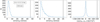 |
Fig. A.1. Error distributions for the bin at R = 11.5 kpc and z = 1.5 kpc for the different velocity components: vR (left), vz (middle), and its covariance (right). The corresponding medians of the error distributions are shown by the vertical grey dotted lines. The vertical grey dashed lines indicate the values of the velocity moments taken from the data directly (i.e. not accounting for the errors). The black vertical solid lines lines show the recovered intrinsic velocity moment from Method 1 (see Sect. 3). Even at this bin, which still contains 2016 stars, the impact of the measurement errors on the recovered velocity moments is relatively small. |
Appendix B: The impact of a systematic parallax offset on the recovered tilt angles
Here we explain how a systematic parallax offset can affect the inferred tilt angles. For this purpose, we now only consider
the (x, z)-plane and we assume that all parallaxes are shifted by the same offset Δϖ = − 0.029 mas.
For Galactic longitude l and latitude b the (U, V, W)-velocities in km s−1 can be computed the usual way (Johnson & Soderblom 1987; Bovy 2011):
 (B.1)
(B.1)
Here, μl⋆ = μl cos(b) and μb denote the proper motions in mas yr−1 in the direction of l and b, respectively, ϖ is the parallax in mas, and  (assuming a Julian year).
When only considering an error in the parallaxes the “observed” velocities are affected as:
 (B.2)
(B.2)
Subscript 0 denotes the true position and velocities, subscript 1 the “observed” quantities. Furthermore:
 (B.3)
(B.3)
and:
 (B.4)
(B.4)
Let us now define the tilt angle δ as:
 (B.5)
(B.5)
In a steady state axisymmetric system ⟨vR⟩ = ⟨vz⟩ = 0. Therefore, at the (x, z)-plane ⟨U⟩ = ⟨W⟩ = 0, and thus var(U) = ⟨U2⟩, var(W) = ⟨W2⟩, and cov(U, W) = ⟨UW⟩. For l = 0° and l = 180° we also notice that U = −vR and W = vz, and therefore that δ = −γ. In the remainder of this appendix we refer to δ when we use “tilt angle” (unless stated otherwise).
Plugging Eq. (B.2) up to first order in  into Eq. (B.5) we get:
 (B.6)
(B.6)
in which:
![Mathematical equation: $$ \begin{aligned} \begin{aligned} \epsilon _A&= \left[ \pm \left(\langle U^2_0 \rangle + \langle W^2_0 \rangle \right) \sin (2b) - 2\langle U_0 W_0 \rangle \right] \left(\frac{\Delta \varpi }{\varpi _0}\right) \\ \epsilon _B&= 2 \left[\langle W_0^2 \rangle \cos ^2(b) - \langle U_0^2 \rangle \sin ^2(b) \right] \left(\frac{\Delta \varpi }{\varpi _0}\right), \end{aligned} \end{aligned} $$](/articles/aa/full_html/2019/09/aa35264-19/aa35264-19-eq35.gif) (B.7)
(B.7)
where ± holds for  .
.
To further explore the effect of a shift in the parallaxes we now investigate what would happen to the tilt angles in two different cases of alignment: spherical alignment and cylindrical alignment.
We start by rewriting Eq. (B.6) into the form of
![Mathematical equation: $$ \begin{aligned} \begin{aligned}&\delta _1 = \frac{1}{2} \arctan \left[ \left( 1+x \right) \tan (2\delta _0) \right] \\&\delta _1 = \delta _0 + \frac{1}{4} \sin (4 \delta _0) \, x + O(x^2) \\&\Delta \delta \simeq \frac{1}{4} \sin (4 \delta _0) \, x . \end{aligned} \end{aligned} $$](/articles/aa/full_html/2019/09/aa35264-19/aa35264-19-eq37.gif) (B.8)
(B.8)
We then get:
![Mathematical equation: $$ \begin{aligned} \begin{aligned} \tan (2 \delta _1)&\simeq \frac{2\langle U_0 W_0 \rangle }{\langle U^2_0 \rangle - \langle W^2_0 \rangle } \left[ \frac{1-\epsilon _{C}}{1 - \epsilon _{D}} \right] \\ \tan (2 \delta _1)&\simeq \tan (2 \delta _0) \left[ \frac{1-\epsilon _{C}}{1 - \epsilon _{D}} \right] , \end{aligned} \end{aligned} $$](/articles/aa/full_html/2019/09/aa35264-19/aa35264-19-eq38.gif) (B.9)
(B.9)
in which:
![Mathematical equation: $$ \begin{aligned} \begin{aligned}&\epsilon _{C} = \left[1 \mp \left( \frac{\langle U^2_0 \rangle + \langle W^2_0 \rangle }{2\langle U_0 W_0 \rangle } \right) \sin (2b)\right] \left(\frac{\Delta \varpi }{\varpi _0}\right) \\&\epsilon _{D} = 2 \left[ \frac{\langle U_0^2 \rangle \sin ^2(b) - \langle W_0^2 \rangle \cos ^2(b)}{\langle U^2_0 \rangle - \langle W^2_0 \rangle } \right] \left(\frac{\Delta \varpi }{\varpi _0}\right) . \end{aligned} \end{aligned} $$](/articles/aa/full_html/2019/09/aa35264-19/aa35264-19-eq39.gif) (B.10)
(B.10)
Then, under the assumptions that |ϵC| ≪ 1 and |ϵD| ≪ 1, we get:
 (B.11)
We highlight the effects for four different latitudes:
![Mathematical equation: $$ \begin{aligned}&b=0^\circ : \quad&x= - \left(\frac{\Delta \varpi }{\varpi _0}\right) \left[ \frac{\langle U^2_0 \rangle + \langle W^2_0 \rangle }{\langle U^2_0 \rangle - \langle W^2_0 \rangle } \right] \nonumber \\&\vert b \vert =90^\circ : \qquad&x= + \left(\frac{\Delta \varpi }{\varpi _0}\right) \left[ \frac{\langle U^2_0 \rangle + \langle W^2_0 \rangle }{\langle U^2_0 \rangle - \langle W^2_0 \rangle } \right] \\&b=+45^\circ : \quad&x= \pm \left(\frac{\Delta \varpi }{\varpi _0}\right) \left[ \frac{\langle U^2_0 \rangle + \langle W^2_0 \rangle }{2\langle U_0 W_0 \rangle } \right] \nonumber \\&b=-45^\circ : \quad&x= \mp \left(\frac{\Delta \varpi }{\varpi _0}\right) \left[ \frac{\langle U^2_0 \rangle + \langle W^2_0 \rangle }{2\langle U_0 W_0 \rangle } \right] \nonumber . \end{aligned} $$](/articles/aa/full_html/2019/09/aa35264-19/aa35264-19-eq41.gif) (B.12)
(B.12)
Since the velocity ellipse is mostly non-tilted (δ0 = 0°) at the Galactic midplane the inferred tilt angles at b = 0° are not affected by an error in the parallax. Geometrically this is not surprising since, at b = 0°, the U-component of the velocities are not affected. The W-velocities are only inflated and do not change the tilt angle. However, if δ0 ≠ 0°, then the term between the square brackets becomes larger than one, since for typical values of the velocity moments at the midplane σ(vR) > σ(vz) (see e.g. Gaia Collaboration 2018c). The inferred tilt angle is therefore steeper (more positive if δ0 > 0° and more negative if δ0 < 0°). At |b|=90°, the effect is reversed and the tilt angle becomes shallower (less positive if δ0 > 0° and less negative if δ0 < 0°) due to the parallax offset. For the case of spherical alignment the relation tan(2δ0) = tan(2θ) can be applied.
The approximations used so far fail for ⟨U0W0⟩≃0, since then  , and for
  , since then
  , and thus
  . In the case of cylindrical alignment (δ0 = ⟨U0W0⟩=0) and for |ϵD| ≪ 1 we get5:
 (B.13)
where we used that tan(2δ1) ≃ 2δ1 for small deviations around δ1 = 0°. This means that at l = 0 (l = 180°) and for σ(vR) > σ(vz) the tilt angles appear to be negative (positive) for b > 0°, and positive (negative) for b < 0°.
We have inserted the relevant Galactic velocity dispersions as a function of R and z and set the covariance term such that there is either spherical or cylindrical alignment throughout the extent of the dataset. We find that the tilt angles are affected very similarly. This is visualised in Fig. B.1 (recall that γ = −δ since we here consider l = 0° and l = 180° only). We therefore think that our test performed in Sect. 5.1 is realistic, even though the intrinsic tilt angles of the GUMS catalogue are more or less cylindrically aligned.
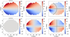 |
Fig. B.1. Effect of a constant shift in the parallaxes of the stars (Δϖ = − 0.029 mas) on the tilt angle γ, as measured in Galactocentric cylindrical coordinates for different types of intrinsic alignment. Left columns: intrinsic tilt angles γ0 as a function of R and z. Middle columns: tilt angles γ1 computed from the “observed” velocity moments. Right columns: Δγ = γ1 − γ0. Be aware of the different colourbar ranges. Top panels: we set the velocity covariances such that the input alignment is spherical. Bottom panels: the input alignment is cylindrical. Black contours denote regions where the tilt angle is not affected, i.e. Δγ = 0°. For spherical alignment this is expected to be the case on the line passing through the Galactic centre and the position of the Sun, thus along z ≈ 0 kpc, and on the circle that goes through the Galactic centre and the position of the Sun. For cylindrical alignment this is expected to occur at both z = z⊙ ≈ 0 kpc and R = R⊙. |
Besides the fact that the orientation of the velocity ellipse changes due to the parallax offset, obviously the stars under consideration also move in position. Thus, in fact a sample of stars with tilt angle δ0 at parallax ϖ0 gets “observed” at ϖ1 with tilt angle δ1. We have not taken this effect into account in the analytic description from this appendix.
All Figures
|
Fig. 1. Star counts from our high-quality Gaia DR2 6D sample in bins of width 1.0 kpc in R and z, as indicated by the box in the upper right corner. The central coordinates of the bins are separated by 0.5 kpc in R and z, thus the bins are not fully independent. The white contours indicate the location of bins with 2000 (inner contour) or 100 (outer contour) stars. The position of the Sun is indicated by the white symbol. Only stars with |
| In the text | |
|
Fig. 2. Velocity ellipses in the meridional plane. The ellipses are colour-coded by their misalignment with respect to spherical alignment. The orientation that corresponds to spherical alignment is indicated by the dotted grey line through each ellipse. The inset in the top right of the figure shows the velocity ellipse for a non-tilted distribution with dispersions σ(vR)=100 km s−1 and σ(vz)=50 km s−1 (see Sect. 4 for more information). The contours show the (relatively small) formal statistical errors on the recovered tilt angles and are drawn for error levels of [0.5, 1.0, 2.0, 4.0] degrees. See Sect. 5 for a discussion on the effect of systematic errors. |
| In the text | |
|
Fig. 3. Tilt angles as a function of Galactic height for different positions across the Galaxy. We show the trends with z for R = [5, 7, 9, 11] kpc. The red squares, green diamonds, and blue crosses are based on the methods described in Sect. 3.2 (see text). The solid black line shows the trend that would correspond to spherical alignment. The tilt angle is changing from spherical alignment in the inner Galaxy (R ∼ 5 kpc) towards shallower tilt angles at R ∼ 11 kpc. The cyan line shows the analytic description of the data as proposed in Sect. 4.4. |
| In the text | |
|
Fig. 4. Velocity ellipses in the meridional plane, now for different positions in azimuth (ϕ = [165 ° ,180 ° ,195 ° ] from top to bottom, respectively). The spatial bins are cubes in (x, y, z), of 1 kpc on a side. The colours of the ellipses represent the misalignment with respect to spherical alignment (as in Fig. 2). |
| In the text | |
|
Fig. 5. Tilt angles as a function of Galactic height for different radial and azimuthal positions across the Galaxy. The red squares, green diamonds, and blue crosses show the measurements for ϕ = [165 ° ,180 ° ,195 ° ], respectively. The black starred symbols show the measurements irrespective of azimuth (as in Sect. 4.1). Given the error bars, there are only small differences in the tilt angles for the different azimuths explored. The solid black line denotes the trend expected for spherical alignment. |
| In the text | |
|
Fig. 6. Velocity ellipses in the meridional plane, as in Fig. 2, but now for the subsamples representing halo (left), thick disk (middle) and thin disk (right) populations. We note that the scaling of the velocity ellipses, indicated by the insets in the bottom right of each panel, are different. The colour coding of the ellipses represents the misalignment with respect to spherical alignment and is the same as in Fig. 2. There is no strong evidence that the tilt angles of the different populations behave differently. |
| In the text | |
|
Fig. 7. Tilt angles as a function of Galactic height for different populations of stars. We show the trends with z for R = 7.5 kpc (top), R = 8.5 kpc (middle) and R = 9.5 kpc (bottom). The red squares, green diamonds, and blue crosses show the results for the halo, thick, and thin disk population described in Sect. 4.3, respectively. The light blue triangles correspond to all LAMOST stars with metallicity information with uncertainties smaller than 0.2 dex, while the black stars are for all stars in the extended sample regardless of whether or not they have metallicity information. The solid black line shows the trend that would correspond to spherical alignment. |
| In the text | |
|
Fig. 8. Left: differences in tilt angles, ΔγGUMS, between error convolved realisations (taking into account random and systematic parallax errors) and the error-free GUMS catalogue. Centre: standard deviation of the tilt angles over all realisations. Right: division of the differences by the corresponding standard deviation. At distances at around 2 kpc the changes are significant with respect to the scatter present between realisations. |
| In the text | |
|
Fig. 9. Tilt angles as a function of Galactic height for different positions across the Galaxy. We show the trends with z for R = [5, 7, 9, 11] kpc for different distance estimates for the stars. The blue squares and orange diamonds use distances based on inverting the parallaxes after correcting the parallaxes for an offset of −29 μas and −54 μas, respectively. The green crosses and red starred symbols use Bayesian distances from McMillan (2018) and Schönrich et al. (2019), respectively. The solid black line shows the trend that would correspond to spherical alignment. |
| In the text | |
|
Fig. 10. Contours of constant prolate spheroidal coordinates, (λ, ν), with foci at R = 0 and z = ±0.88 kpc (see text). Contours of constant λ are shown in blue, contours of constant ν in red. The green ellipses show some of our measured velocity ellipses (Method 1). Their orientation does not align with the coordinate contours at R ≳ 10 kpc and |z|≳2 kpc. |
| In the text | |
|
Fig. 11. Tilt angles for both the Stäckel (purple line) and Piffl et al. (2014, orange line) model for radii at R = 4 kpc and R = 8 kpc (see text). For comparison we add our measurement as green diamonds (Method 1). |
| In the text | |
|
Fig. A.1. Error distributions for the bin at R = 11.5 kpc and z = 1.5 kpc for the different velocity components: vR (left), vz (middle), and its covariance (right). The corresponding medians of the error distributions are shown by the vertical grey dotted lines. The vertical grey dashed lines indicate the values of the velocity moments taken from the data directly (i.e. not accounting for the errors). The black vertical solid lines lines show the recovered intrinsic velocity moment from Method 1 (see Sect. 3). Even at this bin, which still contains 2016 stars, the impact of the measurement errors on the recovered velocity moments is relatively small. |
| In the text | |
|
Fig. B.1. Effect of a constant shift in the parallaxes of the stars (Δϖ = − 0.029 mas) on the tilt angle γ, as measured in Galactocentric cylindrical coordinates for different types of intrinsic alignment. Left columns: intrinsic tilt angles γ0 as a function of R and z. Middle columns: tilt angles γ1 computed from the “observed” velocity moments. Right columns: Δγ = γ1 − γ0. Be aware of the different colourbar ranges. Top panels: we set the velocity covariances such that the input alignment is spherical. Bottom panels: the input alignment is cylindrical. Black contours denote regions where the tilt angle is not affected, i.e. Δγ = 0°. For spherical alignment this is expected to be the case on the line passing through the Galactic centre and the position of the Sun, thus along z ≈ 0 kpc, and on the circle that goes through the Galactic centre and the position of the Sun. For cylindrical alignment this is expected to occur at both z = z⊙ ≈ 0 kpc and R = R⊙. |
| In the text | |
Current usage metrics show cumulative count of Article Views (full-text article views including HTML views, PDF and ePub downloads, according to the available data) and Abstracts Views on Vision4Press platform.
Data correspond to usage on the plateform after 2015. The current usage metrics is available 48-96 hours after online publication and is updated daily on week days.
Initial download of the metrics may take a while.