| Issue |
A&A
Volume 628, August 2019
|
|
|---|---|---|
| Article Number | A26 | |
| Number of page(s) | 14 | |
| Section | Extragalactic astronomy | |
| DOI | https://doi.org/10.1051/0004-6361/201935632 | |
| Published online | 30 July 2019 | |
X-ray occultations in active galactic nuclei: distribution in size of orbiting clouds and total mass content in the cloud ensemble
1
Dipartimento di Fisica e Astronomia, Università di Firenze, Via G. Sansone 1, 50019 Sesto Fiorentino, Firenze, Italy
e-mail: This email address is being protected from spambots. You need JavaScript enabled to view it.
2
INAF – Osservatorio Astrofisico di Arcetri, L.go E. Fermi 5, Firenze, Italy
Received:
5
April
2019
Accepted:
1
June
2019
Abstract
In recent years the short-time X-ray variability of AGNs has been interpreted in terms of varying absorption from the temporary occultation of the primary X-ray source itself owing to the passage of absorbing clouds. Detailed analyses have shown that these clouds are located in the same region and have physical properties similar to those of broad line region (BLR) emitting clouds. The aim of this paper is to investigate in detail whether the same group of orbiting clouds can account for BLR emitting cloud properties and X-ray eclipsing cloud properties as well. To this purpose we looked for a distribution in size for the cloud number density capable of fulfilling the observational requirements of the two groups. The existence of such a distribution not only proves that BLR clouds and eclipsing clouds can be part of the same “family”, but also allows us to estimate the total mass content in clouds orbiting around an AGN black hole.
Key words: galaxies: active / galaxies: Seyfert / X-rays: galaxies
© ESO 2019
1. Introduction
Broad emission lines (BLRs) and X-ray absorption variability are common in active galactic nuclei (AGN). While the origin of broad lines from gas condensations surrounding the central black hole has been examined for a long time (Peterson 2006; Ruff et al. 2012 and references therein), the observed X-ray variability has only recently been ascribed to absorption by a clumpy medium made of clouds orbiting around the central black hole and partially covering the X-ray source when crossing the line of sight to the source itself (see e.g. Risaliti et al. 2007). Several time-resolved spectral studies of a few AGN in hard X-rays performed in recent years on a small number of sources (Risaliti et al. 2009, 2011; Maiolino et al. 2010; Nardini & Risaliti 2011; Puccetti et al. 2007; Bianchi et al. 2009; Sanfrutos et al. 2013) confirm this hypothesis.
From these studies, X-ray obscuring clouds turn out to have a column density NH ∼ 1023 cm−2. Assuming Keplerian motion of the clouds around the central black hole, the typical parameters of the clouds responsible for the broad lines observed in the AGNs optical and ultraviolet spectra can be retrieved. Hence, on the basis of the above-mentioned results, a general scenario for AGN X-ray variability has been proposed: BLR clouds in Keplerian motion temporarily occult the primary X-ray source while crossing the line of sight to the source, thus producing changes in the observed X-ray spectrum and causing its short-term variability.
More recently, the presence and properties of occultations have been analysed in a statistically representative sample of AGN X-ray light curves (Torricelli-Ciamponi et al. 2014, hereafter referred to as Paper I) to estimate how common X-ray eclipses are and whether the properties of the X-ray source and the absorbing clouds inferred from previous studies are general in AGNs. In this framework, the aim of this paper is to test in a more general way whether BLR clouds and X-ray eclipsing clouds belong to the same population. If this is the case, the same population of clouds, interacting with the radiation from the central source, must be capable of producing both the physical phenomenologies, namely capable of both efficiently contributing to broad line formation and absorbing X-rays when occulting the X-ray source. However, even if emission lines and X-ray occultations are originated by clouds that are part of the same “family”, some sort of distribution in physical properties within the family itself must be expected and clouds of different size and located at different distances from the central black hole would have different effects on the central source emission. In fact, for example, clouds located too far from the central source do not receive enough ionising photons to maintain an ionised shell that is efficient in contributing to broad lines emission, whereas the same clouds can produce X-ray eclipses.
In our working scenario, clouds of different sizes exist and they can be located at different distances from the central black hole. This is in agreement with the BLR picture according to which different lines form in clouds located at different distances (see e.g. Kollatschny et al. 2014; Peterson 2006; Peterson & Bentz 2011). Cloud geometry is unknown and indeed it may be far from being very regular. However, a relevant feature regarding the capability of contributing to broad line emission is the extension of the cloud section perpendicular to the radial direction from the AGN centre; this is a measure of the impact area for energetic ionising photons from the central source. In this work, this section is approximated as circular, even though more complex geometries are possible (Maiolino et al. 2010). For simplicity, we assume spherical BLR clouds with radius r in the range r1 ≤ r ≤ r2 and located at about or within distance ∼RBLR so that a portion of each cloud can be ionised.
As for the capability of clouds to produce observable X-ray obscuration effects, again the crucial size is perpendicular to the radial direction to the AGN centre, in this case also perpendicular to the line of sight to the X-ray source, but in this case this size only refers to the cloud “neutral”, X-ray absorbing portion. In our picture, the absorbing neutral portion of the cloud is characterised by its projected radius r, that is the radius of its circular projection on the plane of the sky. We assume that r is in the range r1X ≤ r ≤ r2X and that potentially eclipsing clouds with such a neutral absorbing portion are located in a range of distances from the central black hole between a lower limit ginRBLR and an upper limit gexRBLR, where gin and gex are free parameters. We introduce this parametrisation for the boundaries of the spatial region populated by potentially eclipsing clouds to make it possible to test the effects and potential importance of changing the expected location of the population of clouds capable of producing the eclipse phenomenon with respect to the nominal position of BLR emitting clouds. None of the above parameters is fixed a priori and in principle the possibility of clouds that produce the two distinct phenomenologies (X-ray eclipse and broad line emission) and have the same characteristic size or the same typical position is allowed. For instance, in general the radial dimension of the cloud neutral portion is smaller than that of the whole cloud, i.e. r ≤ r2X < r2. But we can certainly have r2X = r2 in the external region, far from the central source, where ionisation is negligible.
Summarising, in our framework, we suppose that there is a system of cloud-like gas structures (referred to as “clouds” throughout this work) in Keplerian motion in a region around the central black hole and that these clouds can both contribute to broad line emission and produce X-ray occultations, even though we expect efficiently line emitting clouds to be located in the region that we shall define as the proper BLR (see Sect. 2). In contrast the clouds that can act as detectable X-ray occultators are distributed on a range of distances from the AGN centre {ginRBLR, gexRBLR}, which may be more extended than, or may not coincide with, the proper BLR.
In this work our first step is on the one hand to remind the observationally inferred properties of BLR line emitting clouds that are relevant to discuss the scenario above, and, on the other hand, to gather the observationally inferred information on X-ray eclipsing clouds, as it comes from the analysis of Paper I. From these properties, we derive constraints characterising each of the two phenomenological classes of clouds. We then attempt to combine these inferred constraints, demanding that a population of clouds located in a (possibly) rather extended region around the nominal characteristic BLR radius, RBLR, and orbiting around the central black hole with Keplerian velocity, fulfils both classes of constraints. The analysis of the consequences of this requirement may finally give us further insight in the issue of the nature of BLR line emitting and X-ray absorbing clouds, imagining them as a part of a unique greater population with possibly distributed properties.
The paper is organised as follows. Sections 2 and 3 discuss constraints that are relevant to our analysis derived from BLR studies and from the analysis of detected X-ray eclipses, respectively. In Sect. 4 we introduce a distribution in size for all the clouds belonging to the system orbiting around the central black hole, independent of the phenomenology produced by the clouds (contribution to broad line formation or X-ray temporary occultation); we examine and define the characteristics required for such a distribution when we demand that the choice of the distribution and its consequences satisfy both the constraints on BLR clouds and those on clouds capable of eclipsing the AGN X-ray source. In Sect. 5 we derive conditions on the maximum size for a cloud in the adopted distribution, again requiring the fulfilment of the constraints identified in Sects. 2, 3, and 6 combines the results of the previous sections to explore possible further conditions on the cloud population parameters. In Sect. 7 we briefly discuss the type of cloud number density distribution in size that stems from the previous analysis. Section 8 is then devoted to the derivation of an estimate both of the total mass in the global system of clouds and the gas mass content in the BLR; the latter is then compared with a previous estimate of Baldwin et al. (2003). Conclusions are presented in Sect. 9.
For the sake of clarity and for reference purposes, in Appendix B all the parameters introduced and discussed in the present and in the following sections are collected and summarised in Table B.1.
2. Constraints from BLR line emitting clouds
The analysis and diagnostics of broad emission lines (BELs) observations, within the interpretative framework of a BLR consisting of an ensemble of cloud-like single components, allow us to extract information on several physical properties of the clouds and their possible distribution. In the present context, we focus our attention specifically on the following properties, which are relevant to our purposes:
(a) Standard parameter values inferred from modelling the BLR and its observed emission lines are column density NH∼ a few 1022 − 1023 cm−2 (Peterson 2006; Netzer 2015) and number density in the range 108 cm−3 < n < 1012 cm−3 (Baldwin et al. 1995; Korista & Goad 2000; Netzer 2008, 2015; Elvis 2017); coupling these ranges for NH and n, the expected thickness of the gas layer associated with a single cloud should be larger than ∼ a few 1010 cm. Hence, a reasonable condition for the radius r of clouds whose emission contributes to observed lines can be set as r ≳ 3 × 1010 cm. From this we can infer an estimate of the lower limit for the size of a cloud effectively contributing to line emission in the BLR, which in our picture is represented by r1; accordingly, we choose r1 = 3 × 1010 cm.
(b) The global covering factor for the system of BLR clouds, derived in terms of the fraction of the ionising continuum that is converted in line emission, can be evaluated around 30% as a general estimate for any AGN (Baskin & Laor 2018; Maiolino et al. 2001). Also assuming as a zero-order representation of the problem that the ionising radiation is essentially isotropic, this estimate of the BLR covering factor is equal to the geometrical covering factor for the BLR structure. Hence, we adopted a covering factor value Cf ≃ 0.3. Several recent studies on the BLR geometry (see for example Pancoast et al. 2014; Baskin & Laor 2018) suggest a flattened structure rather than a spherical structure.
(c) The number of clouds necessary to originate the observed smooth profile of observed emission lines is high (see Laor et al. 2006). For the few analysed cases in the literature (Laor et al. 2006 and references therein) the estimated cloud number, NTOT, is different for each source: Laor et al. (2006) reported the estimate of NTOT for NGC 4395 as 104 ÷ 105 and mentioned some results from other authors, namely NTOT ≳ 3 × 10⁶ for MRK 335 (Arav et al. 1997) with log(MBH/M⊙)≃7.23 (Bentz & Katz 2015), NTOT ∼ 3 × 10⁷ for NGC 4151 (Arav et al. 1998) with log(MBH/M⊙)≃7.555 (Bentz & Katz 2015), and NTOT ≳ 108 for 3C 273 (Dietrich et al. 1999) with log(MBH/M⊙)≃8.84 (Bentz & Katz 2015). The resulting trend is that sources with a larger central black hole mass, MBH, have a larger number of clouds, which is consistent with the fact that the system dimensions scale with MBH.
(d) The typical distance at which line emitting clouds are present, RBLR, can be related to the mass of the central black hole, MBH, as can be inferred from the analysis of the diagram we obtain by plotting the BLR radius versus the AGN black hole mass for our sample of bright X-ray sources. In fact, for the sources of Paper I sample we derived the value of RBLR from Bentz et al. (2013) radius luminosity correlation, RBLR ≃ 33.65[L5100/1044]0.533 light days (where L5100 ≡ λlλ(erg s−1) at λ = 5100 Å). We adopted, when available, the values of L5100 reported in the literature and, instead, derived L5100 as an extrapolation from the monochromatic 2 keV flux when the value of L5100 was not available in the literature (see Paper I for details). The derived values for log(RBLR) are shown in Fig. 1 as functions of the logarithm of the central black hole mass, MBH, in units of the solar mass, for all the sources of Paper I sample, represented by black dots. The black dots with plotted error bars represent the sources for which we have detected reliable eclipse events in the work described by Paper I and whose corresponding values of log(RBLR) and log(MBH/M⊙) are reported in Table 1 with their uncertainties. The vast majority of the points lie in a strip-like region whose inclination defines a dependence on the central black hole mass, which is  , so that we can infer the following relation:
![Mathematical equation: $$ \begin{aligned} 2.5\times 10^{12}\left[ {M_{\rm BH} \over {M}_{\odot }}\right]^{0.5} \le R_{\rm BLR} \le 4. \times 10^{13} \left[ {M_{\rm BH} \over {M}_{\odot }}\right]^{0.5} \mathrm{(cm)}. \end{aligned} $$](/articles/aa/full_html/2019/08/aa35632-19/aa35632-19-eq2.gif) (1)
(1)
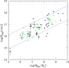 |
Fig. 1. log(RBLR [cm]) as a function of the logarithm of the central black hole mass in units of solar mass. The black points represent the sources of Paper I sample; errors are also plotted for the sources showing reliable X-ray occultations and listed in Table 1. To support our assertion, we also show in green the points referring to AGN sources of the AGN black hole mass database (Bentz & Katz 2015). The two dashed blue lines depict the relationship |

Parameters and derived quantities for sources with reliable occultations detected.
It is significant that, if in order to support our deduction of relation (1) we also plot points referring to other AGN sources for which both MBH and L5100 are available in the literature, again the vast majority of these falls within the same strip defined above; in fact, in Fig. 1 we plot in green the points representing AGN sources of the AGN black hole mass Database of Bentz & Katz (2015) and their distribution does confirm our assertion. Unlike constraints (a)–(c), which are derived from BLR properties well-defined and discussed in the literature, constraint (d) is of a different category (derived by our own analysis of data referring to our bright X-ray sources). Nevertheless, also considering that our analysis is supported and confirmed by the addition of other data available in the literature (see Bentz & Katz 2015, mentioned above), we take constraint (d) and treat it in the same way and at the same level of confidence as constraints (a)–(c).
In the following we describe the geometry for the BLR adopted in this work. To represent and exploit the constraints of point (b), we adopt a schematic description of the structure of the BLR; thus, we suppose that BLR clouds are located and distributed in the region defined by the portion of a sphere of radius ROUT ∝ RBLR subtended by a central angle 2α (where the semi-aperture α is measured from the accretion disc equator), as sketched in Fig. 2. Following Baskin & Laor (2018), for the outer radius ROUT, which is related to the characteristic radius of the BLR, RBLR, we adopt ROUT ≃ 1.5 RBLR. The region where clouds that can effectively contribute to broad line formation are located is indeed also characterised by an inner boundary radius RIN, which we take as RIN ≃ 0.1 RBLR in the following. This choice is qualitatively in agreement with the estimate of RIN ∼ 0.18 RBLR determined by Baskin & Laor (2018); within our present approach, the precise evaluation of the inner boundary of the BLR does not seem to influence our general purposes (as we also verified by changing this boundary in the computations), provided it is not a significant fraction (i.e. close to unity) of RBLR. Assuming an isotropic ionising continuum, null covering in the region outside the BLR and a coverage fraction β0 < 1 within the BLR solid angle, the geometrical covering factor can be evaluated as

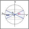 |
Fig. 2. Sketch of the BLR geometry as described in the text. |
since ΩBLR, the solid angle subtended by the BLR region in the chosen geometry, can be expressed as a function of the semi-aperture angle α as
Taking Cf ≃ 0.3 as representative of the BLR covering factor for all AGNs, we can thus derive an estimate of the angle α, depending on the chosen coverage fraction within the BLR, β0, from
 (2)
(2)
so that, with the assumed geometry for the BLR, the representative value for the covering factor Cf = 0.3 (see point (b) of Sect. 2) defines a constrained range for the coverage fraction of the BLR solid angle, β0, that must be 0.3 < β0 < 1 and, more generally,
 (3)
(3)
we choose as representative value β0 = 0.5, obtaining α ≃ 36.9°. In fact, the specific choice of the combination of Cf and α values, within reasonable limits pertaining to the BLR case, does not significantly affect our results in Sects. 5 and 8, as we briefly discuss in those sections.
With this geometrical structure the resulting volume of the BLR is
![Mathematical equation: $$ \begin{aligned} V_{\rm BLR}&= {4\pi \over 3}\left(1.5\,R_{\rm BLR}\right)^3\sin \alpha \left[1-\left({R_{\rm IN}\over R_{\rm OUT}}\right)^3\right]\nonumber \\&\simeq{4\pi \over 3}\left( 1.5\,R_{\rm BLR}\right)^3\sin \alpha , \end{aligned} $$](/articles/aa/full_html/2019/08/aa35632-19/aa35632-19-eq13.gif) (4)
(4)
showing that, with an approximation of less than 0.03%, the introduction of an inner radius for the BLR does not significantly change the global volume.
3. Constraints from X-ray eclipses
We now turn our attention to the reliable eclipse events detected in Paper I. For each of the AGN sources exhibiting such events, in Table 1 we report the number, Necl, of significant (i.e. null probability value Fn < 0.001 and fractional hardness ratio variation ΔHR/HR > 0.1; see Paper I) eclipses as revealed in Paper I, together with the AGN central black hole mass and the RBLR value estimated using the radius-luminosity relation described in the previous section. Table 1 also shows, for each source, our estimate of the maximum cloud size r2, derived in Sect. 5.1, and our evaluation of the BLR mass, MBLR, discussed in Sect. 8.
To extract information from the Paper I analysis and derive constraints on eclipsing clouds, we reiterate our basic assumptions from Paper I. We suppose that each detected eclipse is due to the passage of a single cloud (i.e. a cloud with a neutral X-ray absorbing portion) across the line of sight to the source, that the obscuring cloud is moving with Keplerian velocity, and that the size of the X-ray central source is RX = 2.5 RSchw = 5(GMBH)/c2 as in Paper I. With these assumptions, we proceed to identify constraints on clouds from the analysis of detected X-ray eclipses (Paper I).
First, as its stems from Paper I analysis, for an X-ray temporary occultation event to be reliably classified as an eclipse, the resulting temporary fractional variation of hardness ratio must be ΔHR/HR > 0.1, where HR = F(5 − 10 keV)/F(2 − 4 keV) and F represents the photon flux in the specified ranges. This condition turns out to have consequences on the eclipsing cloud size with respect to that of the X-ray source, RX. In fact, in Paper I we studied the hardness ratio resulting from the convolution of several theoretical model spectra (with varying both X-ray absorbing column density and absorber covering factor) with the response matrices of the X-ray observing instruments (XMM-Newton-EPIC/PN and Suzaku-XIS). From this analysis, for the typical range of absorbing column density values of interest (around 1023 cm−2, see references in Sect. 1), we can relate the observed fractional hardness ratio variation ΔHR/HR to a corresponding estimate of the covering factor of an eclipsing absorber. Taking this into account, the condition for the reliability of a fractional hardness ratio temporary variation as an indicator of an eclipse event, ΔHR/HR > 0.1, implies an eclipse covering factor ≥0.15; this, in turn, can be translated in a condition on the minimum size for the possibly eclipsing cloud, that is r ≳ 0.4 RX. Thus, Paper I condition ΔHR/HR > 0.1 ultimately defines a first constraint for potentially eclipsing clouds, specifically on their minimum size.
Again following the assumptions above, it is also possible to evaluate an eclipsing cloud number density, ρXobs, for each AGN source in Table 1. For each source, a number Necl of reliable occultations were observed during the whole time interval summing up the effective duration of all the observations analysed ΣΔteff; the effective duration of each observation, Δteff is defined as in Paper I.
The total volume of space hosting absorbers that passes across our line of sight to the X-ray source during the total time interval ΣΔteff is
![Mathematical equation: $$ \begin{aligned} V&= (2\,R_{\rm X}) \int ^{g_{\rm ex}}_{g_{\rm in}} \left[\sqrt{ {G~M_{\rm BH} \over g~R_{\rm BLR}}} \Sigma \Delta t_{\rm eff}\right] R_{\rm BLR} \mathrm{d}g\nonumber \\&=4\,R_{\rm X}(GM_{\rm BH})^{1\over 2}\,R_{\rm BLR}^{1\over 2}\Sigma \Delta t_{\rm eff}[g_{\rm ex}^{1/2}-g_{\rm in}^{1/2}],\nonumber \end{aligned} $$](/articles/aa/full_html/2019/08/aa35632-19/aa35632-19-eq14.gif)
where we suppose that (1) eclipsing clouds are endowed with keplerian velocity and (2) eclipsing clouds are located at distances R = gRBLR from the central black hole in the range [ginRBLR]≤R ≤ [gexRBLR]. The inner and outer values of the non-dimensional distance g [≡(R/RBLR)], gin and gex respectively, are taken as parameters of the problem: changing their values allows us to change the location of the region where eclipsing cloud are distributed, so that it is possible to compare their spatial distribution with that predicted for BLR line emitting clouds (for which we would expect gin < 1 and gex ≃ 1). In fact, for instance, the Markowitz et al. (2014) work seems to indicate that in several sources eclipsing clouds are located at larger distances than the typical BLR radius, i.e. gin ≃ 1 and gex > 1.
For each of the sources listed in Table 1, the eclipsing cloud space number density is
![Mathematical equation: $$ \begin{aligned} \rho _{\rm Xobs}\equiv &{N_{\rm ecl} \over V} = \left[{c^2G^{-3/2}\over 20( g_{\rm ex}^{1/2}-g_{\rm in}^{1/2})}\right]\nonumber \\&\times \left[{N_{\rm ecl}\over \Sigma \Delta t_{\rm eff}}\right]\left[R_{\rm BLR}^{-1/2}M_{\rm BH}^{-3/2}\right] ~~ \mathrm{cm}^{-3}, \end{aligned} $$](/articles/aa/full_html/2019/08/aa35632-19/aa35632-19-eq15.gif) (5)
(5)
where the dimensional quantities are expressed in CGS units. In Eq. (5), we have isolated constants and parameters, the eclipse frequency (=Necl/ΣΔteff), and the characteristic AGN source quantities. This obscuring cloud number density is clearly a mean density, averaged over the whole region in which the potentially eclipsing clouds are distributed, defined by the choice of {gin,gex}, regardless of any possible dependence on distance from the central black hole within the region itself. From Eq. (5) it is clear that the values of ρXobs depend on the choice of the region over which we assume eclipsing clouds to be spatially distributed through {gex, gin}. The resulting values of ρXobs, for the sources in Table 1 are plotted as functions of MBH/M⊙ in the log–log graph of Fig. 3 for {gex = 3.0, gin = 0.1}. The uncertainty on log(ρXobs(cm−3)) is evaluated propagating errors on log(MBH/M⊙) and log(RBLR) taken as independent quantities. With this choice of {gex, gin}, the region over which we suppose potentially eclipsing clouds are distributed is more extended than the BLR and contains it entirely. Sources with a more massive central black hole have a lower obscuring cloud number density. The resulting relation ρXobs = ρXobs(MBH/M⊙) can be fitted with a power law, so that it is
 (6)
(6)
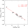 |
Fig. 3. Obscuring cloud number density as it results from the number of observed X-ray occultation events in the case gex = 3.0, gin = 0.1. |
where z is the absolute value of the slope of the linear log–log relationship and where
 (7)
(7)
is the constant term defined as the ratio of a constant A, with the same physical dimensions as ρXobs, to the dependence on the parameters {gex, gin} from Eq. (5). A variation in the choice of the parameters {gex, gin} produces values of ρXobs, which turn out to be fitted with a log–log linear relationship of unchanged slope (−z), but with a “constant” term a0 that changes because of the change in the factor  .
.
Adopting the choice of parameters gin = 0.1 and gex = 3.0, we report and show in Fig. 3 the best fit evaluated by representing our data in the form log(ρXobs) = γ − zx, where  . We fitted the data both with a standard least-squares minimisation technique, and by maximising a modified likelihood which allows for an intrinsic dispersion of the relation; the squared dispersion is added to the variance of each point and fitted as a free parameter. We obtained fully consistent results, in which the intrinsic dispersion is consistent with zero. Since log MBH = 7 is the mean of the logarithmic masses in our sample, the two parameters γ and z have no covariance, so their errors are not correlated. From the fit we obtain γ = −43.4 ± 0.1 and z = 2.00 ± 0.09; the value of a0 in Eq. (6) is thus a0 = −29.4 ± 0.6. From the value derived for a0 and using Eq. (7), we estimate A = 5.6 × 10⁻³⁰ cm−3.
Summarizing, coupling this result with the outcome of Paper I analysis, we can conclude that any cloud producing X-ray occultations must have (at least) the following properties:
(i) The X-ray absorbing portion of the cloud must have a radius, projected on the plane of the sky, r ≳ 0.4 RX; this condition, in fact, defines the lower limit for the projected radius of the X-ray absorbing portion of any eclipsing cloud as r1X = 0.4 RX.
(ii) The cloud must belong to a cloud population whose mean spatial number density (over the whole volume occupied by the cloud system) follows the relationship with the black hole mass shown in Eq. (6).
4. Cloud size distribution
We seek to devise a population of clouds that share both X-ray absorbing cloud and BLR line emitting cloud properties. We wonder whether the constraints defined by BLR emitting cloud properties {(a), (b), (c), (d)} (Sect. 2) are consistent with those following from the properties of clouds producing X-ray occultations, {(i), (ii)} of Sect. 3.
This analysis can be performed only making an assumption on the possible distribution of cloud size. We analyse two possible scenarios:
Case I: in each source clouds of different sizes exist and the cloud size (radius) is monotonically distributed;
Case II: in each source clouds of different sizes exist with a preferred range of cloud radii, so that the distribution has a peak.
The working hypothesis that clouds of different sizes exist in each source is the most reasonable one. We do not address the issue of cloud formation; however, regardless of the expected typical range of size of newly formed clouds, immediately after their birth clouds begin to interact with the external medium. In fact, gravitational and radiative forces act in a different way on the two plasma phases (cloud-intercloud medium), thus generating a relative motion which allows the development of Rayleigh-Taylor instability (Mathews & Ferland 1987). Fast relative motions also induce shocks, which contribute to strip and fragment cloud plasma. Several numerical analyses have been performed on this subject (see e.g. Pittard et al. 2009, 2011), which are all in agreement on the fact that clouds change their shape and size during their probable short life. Therefore, the idea of the simultaneous presence of clouds of different sizes, smaller than the initial one, is perfectly plausible.
A sketch of the two different distributions analysed is shown in Fig. 4. The drawing has free scales, but the ordering of the different relevant radii values is correct. In fact, we have r1 ∼ 3 × 1010cm < r1X = 0.4 RX for all the sources in our sample and it is r2X ≤ r2, as explained in the introduction (Sect. 1).
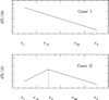 |
Fig. 4. Sketch of possible cloud size distributions. |
We make another simplifying assumption, namely that the distribution of cloud size does not depend on cloud location with respect to the central black hole. This assumption is consistent with the data available from Paper I, which only enable a “mean” ρXobs to be derived; this mean represents an average value on the whole space over which the eclipsing clouds are distributed.
A first test for the two different distributions can be performed by checking whether each of these distributions can fulfil conditions (a), (c), (d) and (i), (ii) of Sects. 2 and 3, respectively. In order to do this, we assume a specific form of cloud distribution in size, dN(r)/dr (number density per unit radius), for the two cases mentioned above and then compute, for each of these, the corresponding average cloud number density for clouds that can produce X-ray occultations, by integrating between the lower and upper limits in size specific for this type of clouds, r1X and r2X (see Sects. 1 and 3), as
 (8)
(8)
This number density should be equal to that inferred from X-ray occultations, ρXobs.
We use this equality, ρ = ρXobs, and the expression derived by the observation fit to Fig. 3 data given in Eq. (6) for ρXobs to determine the distribution normalisation parameter. We can then use dN(r)/dr to estimate the total number of clouds contributing to BLR emission, NTOT, by integrating dN(r)/dr over the whole range of possible radii, {r1, r2}, and over the volume, VBLR, of the BLR region, defined by Eq. (4) in Sect. 2. We obtain
 (9)
(9)
where we used the approximate estimate of the BLR volume VBLR from Eq. (4), where sinα is determined by expression (2) [here α(Cf = 0.3, β0 = 0.5)≃37°]. With this evaluation of NTOT, condition c) on BLR clouds (see Sect. 2) can be tested, also using the expression for RBLR defined by Eq. (1).
In the following we explicitly show the application of this test to the Case I monotonic distribution, while we refer to Appendix A for the discussion of Case II. In fact, the result is that distributions of Case II type in general do not satisfy the constraints identified in Sects. 2 and 3 and therefore such distributions cannot be representative of the physical frame defined by the ensemble of those constraints. The only exception to this conclusion is the Case IIB1 distribution for which the peak occurs (very) close to the lower limit of cloud radii r1 (r1 < r0 < r1X, see Appendix A); however, as discussed in Appendix A, this case is to a large degree equivalent to the monotonic distribution of Case I.
We note that from our analysis we can also exclude the case of a system of clouds of very similar size, or of basically the same size, since such a distribution could be represented as a particular type of Case IIA distribution (see Appendix A), strongly peaked around the specific value of r0 representing the “common” size of the clouds. Such a distribution would not meet the constraints of Sects. 2 and 3, exactly as Case IIA distributions do not.
We now turn our attention to the Case I monotonic distribution of cloud radii. In this scenario we suppose the existence of a cloud number density distribution of the type
 (10)
(10)
where K0 is a normalisation constant and the exponent w is a positive constant parameter; the physical dimension of K0 depends on the actual value of the exponent w and from simple dimensional analysis it is [K0]=[L(w − 4)].
The distribution extends over the range r1 ≤ r ≤ r2. We evaluate a cloud number density to be compared and equated to the observational cloud number density ρXobs, therefore we must select the range of size appropriate to clouds that can produce the X-ray occultations and so must require that r ≥ r1X = 0.4 RX, since smaller clouds would not produce detectable changes in the observed X-ray hardness ratio light curves, and we can reasonably assume r2X = 10 RX. We tested different values for r2X and concluded that final results do not change appreciably for any r2X ≥ 3 RX.
Integrating dN/dr over [r1X, r2X] [see Eq. (8)], we derive the cloud number density referring to clouds that are capable of producing observable occultations of the X-ray source as
 (11)
(11)
then, requiring that this number density is equal to ρXobs, as expressed by relation (6), we have
![Mathematical equation: $$ \begin{aligned} K_0 r_{\rm 1X}^{1-w} {{\left({r_{\rm 2X} \over r_{\rm 1X}}\right)^{1-w}-1} \over 1-w} ={A \over g_{\rm ex}^{1/2}-g_{\rm in}^{1/2}}\left[{M_{\rm BH} \over {M}_{\odot }}\right]^{-z}; \end{aligned} $$](/articles/aa/full_html/2019/08/aa35632-19/aa35632-19-eq24.gif) (12)
(12)
writing r1X = 0.4 RX explicitly with our choice of RX = (5GMBH)/c2 (see Sect. 3), from Eq. (12) we can derive the normalisation constant K0 for the cloud number density distribution, obtaining
![Mathematical equation: $$ \begin{aligned} K_0&={ [(2G{M}_{\odot })/c^2]^{w-1}(w-1)\over 1- (r_{\rm 2X}/r_{\rm 1X})^{(1-w)}}{A\over g_{\rm ex}^{1/2}-g_{\rm in}^{1/2}} \left[{M_{\rm BH} \over {M}_{\odot }}\right]^{w-1-z}\nonumber \\&=D(w) \left[{M_{\rm BH} \over {M}_{\odot }}\right]^{w-1-z}, \end{aligned} $$](/articles/aa/full_html/2019/08/aa35632-19/aa35632-19-eq25.gif) (13)
(13)
where we define
![Mathematical equation: $$ \begin{aligned} D(w) = { [(2G{M}_{\odot })/c^2]^{w-1}(w-1)\over 1- (r_{\rm 2X}/r_{\rm 1X})^{(1-w)}}{A\over g_{\rm ex}^{1/2}-g_{\rm in}^{1/2}} \end{aligned} $$](/articles/aa/full_html/2019/08/aa35632-19/aa35632-19-eq26.gif) (14)
(14)
and where, given our definitions for r1X and r2X in terms of the X-ray source radius RX = RX(MBH), (r2X/r1X) = 25. Once K0 is determined, we can use dN/dr to estimate NTOT by using its expression as defined by Eq. (9). The result is
 (15)
(15)
where the second passage only holds if we suppose w > 1 and if we make the reasonable assumption r2 ≫ r1. If we further take into account the condition on RBLR described by expression (1), we can write
![Mathematical equation: $$ \begin{aligned} {4\pi \over 3}&(1.5)^3\sin \alpha \left\{ 2.5\times 10^{12} \left[{M_{\rm BH} \over {M}_{\odot }}\right] ^{0.5} \right\} ^3 K_0 {r_1^{1-w} \over 1-w} \le N_{\rm TOT} \nonumber \\&\le {4\pi \over 3}(1.5)^3\sin \alpha \left\{ 4\times 10^{13} \left[{M_{\rm BH} \over {M}_{\odot }}\right] ^{0.5} \right\} ^3 K_0 {r_1^{1-w} \over w-1}, \end{aligned} $$](/articles/aa/full_html/2019/08/aa35632-19/aa35632-19-eq28.gif) (16)
(16)
where K0 and r1 must be thought as expressed in CGS units, since relation (1) defines the limits on RBLR in cm and as a consequence the numerical coefficients 2.5 × 10¹² and 4 × 10¹³ are also values in cm. As ![Mathematical equation: $ K_0\propto [{M_{\mathrm{BH}} \over {M}_{\odot}}]^{w-1-z} $](/articles/aa/full_html/2019/08/aa35632-19/aa35632-19-eq29.gif) , expression (16) implies that
, expression (16) implies that
 (17)
(17)
and hence its value can increase, with increasing MBH, as requested by condition c) of Sect. 2, provided
 (18)
(18)
If condition (18) is fulfilled, the choice of the monotonic distribution and its consequences comply both with properties (a), (c), (d) relative to BL emitting clouds and with properties (i), (ii) for clouds capable of eclipsing the X-ray source.
5. Maximum cloud size
Taking into account the results of the previous section and Appendix A, we assume now a monotonic distribution of cloud radii to describe both BLR clouds and X-ray eclipsing clouds. We derive an approximate estimate of the covering factor of BLR line emitting clouds using Eq. (10) for dN/dr and the expressions following from this equation in Sect. 4 and by taking into account the assumptions on the BLR geometry mentioned in Sect. 2. We can then require that this approximate covering factor of BLR line emitting clouds is in agreement with the representative “universal” value representing condition (b) of Sect. 2, that is
![Mathematical equation: $$ \begin{aligned} 0.3&\simeq C_{\rm f}= \int ^{R_{\rm OUT}}_{R_{\rm IN}} \int ^{r_{2}}_{r_{1}} \pi r^{2}{\mathrm{d}N\over \mathrm{d}r} \mathrm{d}r {\mathrm{d}V_{\rm BLR}(R)\over 4\pi R^2}\\&= \pi \sin \alpha (R_{\rm OUT}-R_{\rm IN})K_0{r_2^{3-w}\over 3-w}\left[1-\left(r_1\over r_2\right)^{3-w}\right], \end{aligned} $$](/articles/aa/full_html/2019/08/aa35632-19/aa35632-19-eq32.gif)
where dVBLR = 4πsinαR2dR.
Recalling our choices for ROUT ≃ 1.5 RBLR and RIN ≃ 0.1 RBLR, we can write the expression above as
![Mathematical equation: $$ \begin{aligned} 0.3\simeq C_{\rm f}= 1.4~\pi \sin \alpha ~ R_{\rm BLR} K_0{r_2^{3-w}\over 3-w}\left[1-\left(r_1\over r_2\right)^{3-w}\right], \end{aligned} $$](/articles/aa/full_html/2019/08/aa35632-19/aa35632-19-eq33.gif) (19)
(19)
where r1 = 3 × 1010 cm (as in discussed in condition (a) of Sect. 2) and K0 is the normalisation constant given by Eq. (13). Since our choice of the geometry of the BLR described in Sect. 2 gives sinα = Cf/β0 [Eq. (2)], the value of the covering factor Cf cancels out in Eq. (19); however, the specific value of Cf that is adopted still affects Eq. (19) in that it constrains the range of the BLR solid angle coverage fraction β0, as defined by condition (3), Cf < β0 < 1. In the computations we present we chose to adopt the representative value Cf = 0.3 [according to constraint b) of Sect. 2] and β0 = 0.5.
Provided the following conditions are satisfied,
 (20)
(20)
we use Eq. (19) to derive r2 as
![Mathematical equation: $$ \begin{aligned} r_2= \left[{(3-w)\beta _0\over 1.4\pi }\right]^{1/(3-w)}\left(R_{\rm BLR}K_0\right)^{1/(w-3)}, \end{aligned} $$](/articles/aa/full_html/2019/08/aa35632-19/aa35632-19-eq35.gif) (21)
(21)
defining an estimate of the upper limit of the cloud size range, r2, as a function of the quantities K0, RBLR, w.
In Sect. 4 we identified two conditions on the slope w of dN/dr, namely w > 1 and z − 0.5 < w < 3; for the value z = 2.00 derived from the fit of the relation between ρXobs and MBH (see Eq. (6)), these conditions can be safely summarised as
 (22)
(22)
5.1. Sources of our sample
For each source listed in Table 1 the normalisation constant K0 can be derived equating Eq. (11) to the value of ρXobs derived from Eq. (5). We obtain
where we have r1X = 0.4 RX and r2X = 10 RX. Using the expression above for K0 and the values of RBLR given in Table 1, r2 can be computed from Eq. (21). The resulting values for the cloud maximum possible extension, for the case w = 2.0, gin = 0.1 and gex = 3, are reported in Table 1 and shown as green points in Fig. 5.
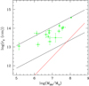 |
Fig. 5. Allowed range for the upper limit for cloud size distribution, r2, is shown as a function of MBH (black lines) as derived in Eq. ( 23) for the cases w = 2.0, z = 2.00, and {gex = 3.0, gin = 0.1}. The red line shows the lower limiting condition on r2, again as a function of MBH, holding for sources in whose light curves we detected reliable X-ray eclipses and defined by Eq. (26). Green points show the values of r2 directly computed according to the procedure described in Sect. 5.1 for the sources of Table 1. See the text for details. |
5.2. General formulation
If the relationship, defined by expression (6) and Fig. 3 holds for any AGN whose central region hosts a system of clouds in motion around the central black hole, then limits on the BLR maximum size, r2, can be derived. With this assumption, we can use the general expression for K0 (Eq. (13) of Sect. 4) in Eq. (21) to derive the upper limit of r2.
We can extend the constraints on RBLR (defined by Eq. (1)) to any AGN with a BLR cloud system. This is a reliable choice since, as apparent Fig. 1, the definition of upper and lower boundaries of the strip-like region in a log–log plot, where virtually all the points {RBLR, MBH} representing the sources in the sample of Table 1 are located, applies to all the points for AGNs with estimates of RBLR and MBH available in the literature (see Bentz & Katz 2015).
Using Eq. (13) for K0 and Eq. (1) constraining the values of RBLR, Eq. (21) gives a range of acceptable values for r2, the upper limit of the cloud size range
![Mathematical equation: $$ \begin{aligned} \left[{2.5\times 10^{12} \over B(w)} \left({M_{\rm BH} \over {M}_{\odot }}\right)^{w-0.5-z}\right]^{1\over w-3} &\ge r_2~(\mathrm{cm}) \nonumber\\ &\ge \left[{4\times 10^{13} \over B(w)} \left({M_{\rm BH} \over {M}_{\odot }}\right)^{w-0.5-z}\right]^{1\over w-3 }\end{aligned} $$](/articles/aa/full_html/2019/08/aa35632-19/aa35632-19-eq38.gif) (23)
(23)
where we define
![Mathematical equation: $$ \begin{aligned} B(w)&={\beta _0\over 1.4~\pi }~{3-w \over w-1}~{1-(r_{\rm 2X}/r_{\rm 1X})^{1-w} \over [(2G{M}_{\odot })/c^2]^{w-1} }{g_{\rm ex}^{1/2}-g_{\rm in}^{1/2} \over A }\nonumber \\&={\beta _0(3-w)\over 1.4~\pi }{1\over D(w)} \end{aligned} $$](/articles/aa/full_html/2019/08/aa35632-19/aa35632-19-eq39.gif) (24)
(24)
and D(w) is given by Eq. (14). As in relation (16), the numerical coefficients are values in cm and hence all the physical quantities are in CGS units. Equation (23) shows that the value of r2 depends on the choice of the parameters w, z, gex, and gin. The value of the upper limit of cloud radius, r2, is crucial to this computation, since large clouds give a strong contribution to the global BLR covering factor (even though only a small shell of the cloud is ionised and contributes to line emission).
Figure 5 illustrates the range of r2 values determined by Eq. (23) as a function of MBH for a specific choice of the parameters, namely w = 2.0, z = 2.00, gin = 0.1, and gex = 3.
Expression (23) shows that r2 increases with MBH if [(w − 0.5 − z)/(w − 3)] > 0. Considering condition (22) we obtain w − 0.5 − z < 0. Therefore, the range for w values that also ensures an increase of r2 with increasing MBH would be further restricted to
 (25)
(25)
The estimates of r2 for all of the sources listed in Table 1 are shown in Fig. 5 as green circles and they turn out to be consistent with the range of values allowed by the constraint defined by expression (23). In addition, as explained in Sect. 3, X-ray eclipses can be observed only if the cloud size, r, is large enough, specifically if r ≥ r1X = 0.4 RX. This condition must apply even more strictly to r2. The corresponding absolute minimum value of r2 is shown as a red line in Fig. 5 as a function of MBH. All the estimates of r2 for the sources of Table 1 sample are consistent with this condition (see Fig. 5). The region of the plane (log(MBH/M⊙),log(r2)) to the right of the red line itself corresponds to clouds that do not allow an observable and reliable X-ray eclipse. In Fig. 5, with the specific choice adopted for the parameters of the problem ({w = 2, gex = 3.0, gin = 0.1}) and with our choice for β0 (β0 = 0.5), the red line intersects the estimated range for r2 when MBH/M⊙ > 107.9 and with MBH further increasing, there is a decrease in the range of corresponding possible r2 values that are compatible with the condition of existence of clouds capable of producing observable X-ray eclipses. This is consistent with the observational lack of X-ray eclipses detections for MBH > 108.05 M⊙ in our analysis of Paper I.
Changing the assumed value of the parameter β0 within the range Cf < β0 < 1, both the values of r2 for the sources and the upper and lower limiting conditions on r2, defined by Eq. (23), are modified by the same factor (since  in both cases). The effect in Fig. 5 is just a global upward shift (for an increase of β0) or downward shift (for a decrease of β0) of the whole system of points and limiting condition lines. For instance, using β0 ≃ 0.3, the lowest possible value of β0 for Cf ≃ 0.3 (implying α ≃ 90°, i.e. a spherical BLR), source points and black lines in Fig. 5 (drawn for w = 2) would be all shifted downwards by log(0.5/0.3)≃0.22. On the contrary, the red line defining the limiting condition for occultation effects detectability of course remains unchanged; therefore, a decrease in β0 would produce a decrease of the black hole mass at which the red line starts to intersect the region of possible values for r2 and viceversa. Nevertheless, even in the limiting case of the example above (β0 ≃ 0.3) all the points representing our eclipsed sources would consistently remain well above the red line.
6. Defining a range for the cloud size distribution exponent w
Figure 5 shows the results for a specific set of free parameters. It is interesting to investigate how the results of Fig. 5 change, when varying the parameters values and also to investigate the range of w for which the BLR and X-ray eclipsing clouds can be the same. In this section we discuss the results maintaining β0 = 0.5.
The sources for which X-ray eclipses have been observed must be surrounded by clouds of size r ≥ r1X = 0.4 RX (condition (i) of Sect. 3) Hence, noting that RX = 2.5 RS ≃ 7.4 × 10⁵(MBH/M⊙) cm, the maximum cloud size r2, must satisfy the condition
![Mathematical equation: $$ \begin{aligned} r_2> 2.96\times 10^5 \left[{M_{\rm BH} \over {M}_{\odot }}\right]\,\mathrm{cm}. \end{aligned} $$](/articles/aa/full_html/2019/08/aa35632-19/aa35632-19-eq42.gif) (26)
(26)
The maximum value for r2, r2M(MBH) (defined by expression (23)), must thus be larger than this limiting value. In the (MBH, r2) plane for any value of MBH, this condition is expressed as
![Mathematical equation: $$ \begin{aligned} r_{\rm 2M}\equiv \left\{ {2.5\times 10^{12} \over B(w)}\left[{M_{\rm BH} \over {M}_{\odot }}\right]^{w-0.5-z}\right\} ^{1\over w-3}\ge 2.96\times 10^5 \left[{M_{\rm BH} \over {M}_{\odot }}\right] , \end{aligned} $$](/articles/aa/full_html/2019/08/aa35632-19/aa35632-19-eq43.gif) (27)
(27)
where r2M is again expressed in cm. The limiting condition is the intersection between the two curves
![Mathematical equation: $$ \begin{aligned} \left\{ {2.5\times 10^{12} \over B(w)}\left[{M_{\rm BH} \over {M}_{\odot }}\right]^{w-0.5-z}\right\} ^{1\over w-3} =2.96~10^5 \left[{M_{\rm BH} \over {M}_{\odot }}\right]\cdot \end{aligned} $$](/articles/aa/full_html/2019/08/aa35632-19/aa35632-19-eq44.gif) (28)
(28)
This can be cast into a limiting condition for the parameter z as a function of w, gex, and gin, where the latter two parameters appear in B(w), Eq. (24), for any given value of MBH, i.e.
![Mathematical equation: $$ \begin{aligned} z= { [5.47~(3-w)+12.40-\log (B(w))]\over \log \left({M_{\rm BH}/ {M}_{\odot }}\right)}+2.5. \end{aligned} $$](/articles/aa/full_html/2019/08/aa35632-19/aa35632-19-eq45.gif) (29)
(29)
From this relation we can derive the limiting curves w = w(z), in the (z, w)-plane, for each choice of the parameters {gex, gin} and of MBH. In Fig. 6 these limits are plotted for MBH ≃ 1.12 × 10⁸ M⊙. This is the largest mass value among the sources in Table 1. The curves are derived for different values of gex and gin.
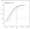 |
Fig. 6. Limits for the values of parameter w as a function of z for the case log(MBH/M⊙) = 8.15. The black dotted lines show the limits defined by condition (25); the vertical blue dashed line represents z = 2.00, which is our fit value of the slope for log(ρXobs) as a function of log(MBH/M⊙) defined by Eq. (6). The curves w = w(z) are derived from condition (29) for different choices of the parameters {gex, gin} characterising the region in which eclipsing clouds are located; the various cases shown are identified by the following code: black refers to gex = 3.0, the solid line indicates gin = 0.1, the dashed line refers to gin = 0.3, dot-dashed line indicates gin = 0.8, and red refers to gex = 1.5; the gin values have same line-type code. The region of allowed values for w is between the two black dotted lines and on the right of the w(z) curve for each case. |
We are interested in values z < 2.5 (from our fit it is z = 2.00, see Sect. 2). Only z values larger than that obtained from relation (29) satisfy condition (27) and, as a consequence, the “allowed” region in the w − z plane is to the right of the curve w(z) that can be derived from Eq. (29). The largest black hole mass in Table 1 corresponds to the most restrictive condition for w as a function of z in the (z, w) plane.
The case z = 2.00 (see Fig. 3, Sect. 3) is shown in Fig. 6 as a vertical dashed blue line. Figure 6 also shows two dotted black lines, obtained from condition (25) and representing the lower and upper limits on w. For the lower limit, the condition comes from the requirement for NTOT to be increasing with increasing MBH. For the upper limit, the condition comes from r2 increasing with black hole mass.
The intersection of z = 2.00 with the lower and upper limits on w (dotted black lines) defines a range for w: 1.5 < w < 2.5. The most limiting curve w(z) among those drawn in Fig. 6 (corresponding to gin = 0.8, gex = 1.5) intersects the vertical line z = 2.00 at w ≃ 2.5 and defines the same range of allowed values for w. Larger values of gin, that is even narrower ranges of distances for the spatial distribution of potentially eclipsing clouds, would lead to an effective upper limit for w smaller than 2.5; the value is derived from condition (25).
Therefore, provided gin ≤ 0.8, then for 1.5 < w < 2.5, the same distribution for the cloud size can be adopted for all the sources in Table 1, independent of the location of the region where the X-ray eclipsing clouds are distributed.
Hence, apart from the condition gin ≤ 0.8, no further information on the location of X-ray absorbing clouds can be inferred. In the Markowitz et al. (2014) study of a dozen of eclipse events detected in eight sources, the distance of eclipsing clouds corresponds to the external border of the BLR or even farther in several cases. On the basis of the present analysis, we cannot comment on the location of eclipsing clouds. The issue of the location of these clouds will be addressed in more detail in a forthcoming paper.
7. Cloud distribution
The w = 2 distribution in cloud size is shown in Fig. 7 for two different values of the central black hole mass and for the case w = 2.0, gex = 3, and gin = 0.1, where K0 is given by Eq. (13). The whole extent of the line (both dashed and solid portions) represents clouds which contribute to BLR emission, i.e. clouds with 3 × 1010 cm ≤ r ≤ r2M. The solid line shows the part of the cloud distribution that contributes to both BLR emissions and to detectable X-ray eclipsing clouds.
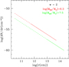 |
Fig. 7. Cloud distribution for w = 2.0, gex = 3. and gin = 0.1 for two different black hole masses: MBH ≃ 2 × 10⁶ M⊙ in red and MBH ≃ 3.2 × 10⁷ M⊙ in green. For each MBH value, all the clouds in the entire size range shown in the figure can contribute to broad line formation, whereas only the portion of the distribution drawn as a solid line corresponds to clouds potentially producing X-ray occultations. |
The different values of the black hole mass show how K0 and the maximum allowed r2 value, r2M [condition (27)], change for different central black hole mass values. The larger the central black hole mass is, the smaller the number density of potentially eclipsing clouds.
The form of the distribution also induces another selection effect decreasing the number of observed occultations. Assuming that w ≃ 2 is a reasonable value for the absolute value of the distribution slope, the number density of the smallest “observable” X-ray eclipsing clouds is [(0.4 RX)/(10 RX)]1 − w ∼ 25, i.e. ∼25 times larger than the number density of clouds with r = 10 RX. Hence, the detection of X-ray eclipses produced by large clouds is disfavoured because large clouds are far less common and demand long observation times to be revealed.
8. Total mass in orbiting clouds
A large portion of the cloud distribution (the one represented by the dashed line in Fig. 7) does not contribute to detectable X-ray occultations. Therefore the cloud density ρXobs (Sect. 3) does not represent the total cloud density. To derive the total mass both of the clouds of the proper BLR (MBLR) and of the whole ensemble of orbiting clouds (Mcloud), the entire range of radius, r1 ≤ r ≤ r2, must be taken into account.
The total mass in BLR orbiting clouds can then be derived integrating the cloud distribution
 (30)
(30)
where n is the gas number density in each cloud, mH is the hydrogen atom mass, and  (Eq. (4) of Sect. 4) is the volume of the BLR, where clouds significantly contributing to broad line formation are located. We thus obtain
 (31)
(31)
where we required r2 ≫ r1 and z − 0.5 < w < z + 0.5.
For the sources in Table 1 we estimate MBLR, the mass in BLR line emitting clouds, with Eq. (31), making use of RBLR (values in Table 1) and of K0 (Sect. 5.1). For the gas number density of BLR clouds, n, given that the characteristic values typically reported in the literature are n = 1010 cm−3 or 1011 cm−3 (see e.g. Elvis 2017; Netzer 2013; Peterson 1997, 2006; Schnorr-Müller et al. 2016), we choose n = 5 × 1010 cm−3 (see also Baskin & Laor 2018). We also assume {gex = 3, gin = 0.1, w = 2.0} and sinα = 0.6, following from the assumption of Cf ∼ 0.3 (as required by condition (b) of Sect. 2) and the choice of β0 = 0.5 (see Eq. 2 of Sect. 2). The values of MBLR that we have thus derived for our sources are listed in Table 1. The uncertainty on log(MBLR/M⊙) is evaluated propagating errors on the two basic physical quantities that we consider as independent, log(RBLR) and log(MBH/M⊙).
An independent estimate of BLR cloud mass is based on the observed luminosity of emission lines. The method only takes into account the ionised part of the gas in the clouds. Baldwin et al. (2003) compared different expressions present in literature and performed a detailed analysis, obtaining an estimate for the mass of the ionised plasma in the BLR, i.e.
 (32)
(32)
where l1450 is the monochromatic luminosity at 1450 Å, in erg s−1 Å−1. To compare the Baldwin et al. (2003) results with the BLR cloud mass MBLR obtained with our method, we derived l1450 for each source of Table 1, from the source 5100 Å luminosity, L5100(erg s−1), adopting for this the value present in the literature, when available (Winter et al. 2010; Bentz et al. 2013), or, otherwise, evaluating L5100 with the method described in Sect. 5 of Paper I and using the optical-to-Xray spectral index given by Young et al. (2010). With L5100(erg s−1), we determined l1450(erg s−1 Å−1) as
and then we used this estimate of the specific luminosity l1450 in Eq. (32). The range of BLR clouds mass values thus obtained for each source of Table 1 is shown in Fig. 8, represented as a dashed green vertical bar.
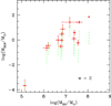 |
Fig. 8. Values of the total mass in BLR clouds as a function of MBH for gex = 3.0, gin = 0.1 and w = 2.0. Green vertical bars show the BLR mass range estimated according to the relation of Baldwin et al. (2003) derived from line emission. |
The estimates of MBLR (Table 1) are shown as red points in Fig. 8. These values are generally consistent with the range derived from Baldwin et al. (2003). Our estimates are higher or lie close to the upper limit of the Baldwin et al. (2003) range. This result is expected, since the Baldwin et al. (2003) analysis takes into account only the mass of the ionised gas, while in our computation the whole amount of gas in each cloud is considered.
For values of w corresponding to r2 decreasing with increasing MBH (z + 0.5 < w < 3, see Sect. 5.2), the resulting values of MBLR would show a distribution inconsistent with the estimates from Baldwin et al. (2003) relation.
As for possible effects of BLR covering factor, Cf, and/or of BLR geometrical parameters variations (see Sect. 2) on our estimates of MBLR for the sources of Table 1, we note that from Eq. (31),

Thus, for instance, a decrease of Cf value by a factor of 2 (from Cf = 0.3 to Cf = 0.15), maintaining β0 = 0.5, would produce a decrease by the same factor in MBLR values; however, this would have the side effect of changing the BLR half-opening angle to α ∼ 17.5°. If, on the contrary, we choose to keep α unchanged (≃36.9°, as in Sect. 2), assuming Cf = 0.15 would require β0 = 0.25 and, maintaining w = 2, our estimates of MBLR would all be decreased by a factor of 4 (shifting downwards by ∼ − 0.6 in Fig. 8). In both cases, the outcome of our comparison with Baldwin et al. (2003) results would not be affected because our estimates would still be consistent with Baldwin et al. (2003) estimated ranges.
We can also derive Mcloud, the total mass in the whole ensemble of orbiting clouds, which can be distributed on a region more extended that the proper BLR, if gex > 1.5 = (ROUT/RBLR); for our present choice, where gex = 3, this is just the case. To evaluate Mcloud, we use again the same form of Eq. (30), but substitute VBLR with the volume VTOT of the entire region over which the whole system of clouds (producing whatever physical effect) are spatially distributed; this is, in its most general form,
![Mathematical equation: $$ V_{\rm TOT}= \left({4 \over 3} \pi \sin \alpha \right) R_{\rm BLR}^3\left[\left(R_{\rm max}\over R_{\rm BLR}\right)^3-\left(R_{\rm min}\over R_{\rm BLR}\right)^3\right] , $$](/articles/aa/full_html/2019/08/aa35632-19/aa35632-19-eq52.gif)
where Rmax ≡ max{ROUT, gexRBLR} and Rmin ≡ min{RIN, ginRBLR} With the exemplifying choice adopted throughout the computations in the previous sections, {gin = 0.1, gex = 3} and {RIN/RBLR = 0.1, ROUT/RBLR = 1.5}, it is Rmin = 0.1 RBLR and Rmax = 3 RBLR; we thus also include a region “external” to the BLR. In this region, we assume clouds to be still present, but not significantly contributing to broad line formation, whereas possibly capable of producing occultations (see Sects. 3 and 4). Our general expression for the total mass in the global system of orbiting clouds is then
![Mathematical equation: $$ \begin{aligned} M_{\rm cloud}= \left({16 \over 9} \pi ^2 \sin \alpha \right) \left[\left(R_{\rm max}\over R_{\rm BLR}\right)^3-\left(R_{\rm min}\over R_{\rm BLR}\right)^3\right]R_{\rm BLR}^3 ~m_{\rm H} n~ K_0{r_2^{4-w}\over 4-w}, \end{aligned} $$](/articles/aa/full_html/2019/08/aa35632-19/aa35632-19-eq53.gif) (33)
(33)
with the same conditions assumed for Eq. (31), r2 ≫ r1, z − 0.5 < w < z + 0.5 and sinα = 0.6, for our choice of parameters, {gin = 0.1, gex = 3}, we have Mcloud ≃ 8MBLR.
For NGC 1365 we can also compare our result with the value of the mass in absorbing clouds Mabs ≃ 0.004 M⊙ derived by Maiolino et al. (2010) in their analysis of the source X-ray occultations. We obtain a much larger value, Mcloud ≃ 7.9 M⊙, since our derivation from the overall cloud distribution takes into account all the clouds orbiting around the black hole and not only the X-ray occulting clouds.
We can also derive a more general expression both for the total mass amount in orbiting clouds, Mcloud, and for MBLR, substituting, in Eqs. (33) and (31), respectively, for r2 using Eq. (21), for K0 using Eq. (13), and for RBLR with expression (1) constraining its values as a function of MBH. The result of these substitutions is that both the total mass in clouds and the mass in clouds of the BLR proper show the same behaviour with MBH, that is
 (34)
(34)
where
taking into account condition (25) on w, for any w in that range the exponent δ of the ratio (MBH/M⊙) is positive (for w = 2, the exponent value is δ = 1.50). This is indeed a reasonable inference and a BLR mass increasing with MBH is in good agreement with the trend of the estimate of the BLR mass content given by Baldwin et al. (2003), as can be seen from the exemplifying Fig. 8.
9. Conclusions
In this paper we have tested whether an ensemble of clouds orbiting around the central black hole can produce both large emission lines observed in AGN spectra and obscuration of the central X-ray source, thus inducing the X-ray observed variability in the hardness ratio. Starting from this scenario, we required its compatibility with constraints defined both by BLR properties and observed X-ray occultations and explored the consequences of this request on a first physical description of the global cloud system orbiting the central black hole. The main results of this work are the following:
-
We found that the scenario above is viable if clouds follow a distribution in radius, r, which is monotonic in shape (or monotonic except for low cloud radii, where a peak may exist). Therefore the idea that the same clouds are at the origin of both the observed features, broad lines in the UV-optical spectra and short time variability in the X-rays, seems to be reliable. We have found that, for a monotonic distribution in cloud size of the type ∼r−w to be actually descriptive of the problem, the exponent w must be in the range 1.50 < w < 2.50.
-
Exploiting the results of the X-ray occultation search performed in Paper I, the number density of occulting clouds, derived from detected X-ray occultations for the sources of our sample, turns out to decrease with increasing black hole mass (see Fig. 3); this anti-correlation has proved to be a strong constraint to get information about the cloud size distribution. In fact, the derived trend
 is strictly linked to the existence of a lower limit to the radius of a cloud that can be deemed to be observable with the method of X-ray occultations described in Paper I. Indeed, the specific procedure of this method prevents the detection of clouds with radius smaller than ≃0.4 RX. Hence, there is a sort of selection effect related to the value of MBH. This fact is apparent in Fig. 7 where the solid line portion of each distribution shown identifies the range of radius for clouds with size suitable for producing X-ray occultations. In the case of the larger black hole mass most clouds are too small for their passage across the line of sight to the X-ray source to be detected as a reliable X-ray eclipse, and those which in principle are detectable as X-ray occultators are by far less abundant.
 -
In this analysis we also found that, for each central mass MBH, a maximum possible cloud extension, r2M, exists and this does not scale linearly with MBH. Since typical AGN scale dimensions are linked to the Schwarzschild radius RSchw, i.e. to MBH, this result suggests that the cloud size also depends on other physical parameters of gas clouds, such as gas density and temperature, which appear to assume values in a rather narrow range in any AGN BLR (Osterbrock & Ferland 2006); this may affect the maximum extension of clouds modifying the simple linear scaling with MBH.
-
The cloud distribution in size derived from our analysis allows the evaluation of the global amount of gas in orbiting clouds, independent of the phenomenology that they produce (line emission or X-ray eclipse). The resulting values for the gas content in the spatial region from which the contributions to broad line emission arise (as shown in Sect. 8) turn out to be compatible with the upper limit of the range derived from line analysis by Baldwin et al. 2003 or slightly larger than that. This is consistent with the fact that in the present line of work we also include the neutral portion of each cloud in the computation.
The aim of the present analysis was restricted to the assessment of the global and general properties of the system of orbiting clouds that can both contribute to the emission of broad lines and produce temporary X-ray source occultations. Our conclusion is that indeed such a system of clouds can exist with the above characteristics, but more detailed study is of course required.
From the analysis of AGN X-ray spectral properties an estimate of the X-ray absorbing neutral gas column density NHX can be inferred (Bianchi et al. 2012). The resulting value is in the range [5 × 10²² ÷ 2 × 10²³] cm−2, defining the mostly neutral portion of the cloud. For a given cloud the actual value of NHX depends on the cloud ionisation condition. If clouds are located at a distance ≳RBLR, they only have a thin ionised layer, while for clouds located at distances < RBLR only a small portion of the cloud would be neutral. Therefore, the value of NHX depends on the actual cloud distance from the central black hole. The introduction of two more variables, i.e. the neutral portion column density, NHX, and the cloud distance, in our investigation cannot be addressed without the inclusion of the ionisation balance for the gas clouds in the analysis. In this framework it is consistent that the present analysis can give no information regarding the dependence of cloud properties on the spatial location. This point will be addressed in a forthcoming paper. All the above conclusions hold for all the sources for which X-ray eclipses have been observed, but they can be extended to all AGN sources showing BLR emission even though no X-ray eclipse has been detected.
Acknowledgments
We acknowledge financial contribution from the agreement ASI-INAF n.2017-14-H.O
References
- Arav, N., Barlow, T. A., Laor, A., & Blandford, R. D. 1997, MNRAS, 288, 1015 [NASA ADS] [CrossRef] [Google Scholar]
- Arav, N., Barlow, T. A., Laor, A., Sargent, W. L. W., & Blandford, R. D. 1998, MNRAS, 297, 990 [NASA ADS] [CrossRef] [Google Scholar]
- Baldwin, J., Ferland, G., Korista, K., & Verner, D. 1995, ApJ, 455, L119 [NASA ADS] [CrossRef] [Google Scholar]
- Baldwin, J. A., Ferland, G. J., Korista, K. T., Hamann, F., & Dietrich, M. 2003, ApJ, 582, 590 [NASA ADS] [CrossRef] [Google Scholar]
- Baskin, A., & Laor, A. 2018, MNRAS, 474, 1970 [NASA ADS] [CrossRef] [Google Scholar]
- Bentz, M. C., & Katz, S. 2015, PASP, 127, 67 [NASA ADS] [CrossRef] [Google Scholar]
- Bentz, M. C., Denney, K. D., Grier, C. J., et al. 2013, ApJ, 767, 149 [NASA ADS] [CrossRef] [Google Scholar]
- Bentz, M. C., Cackett, E. M., Crenshaw, D. M., et al. 2016, ApJ, 830, 136 [NASA ADS] [CrossRef] [Google Scholar]
- Bianchi, S., Piconcelli, E., Chiaberge, M., et al. 2009, ApJ, 695, 781 [NASA ADS] [CrossRef] [Google Scholar]
- Bianchi, S., Maiolino, R., & Risaliti, G. 2012, Adv. Astron., 2012, 782030 [NASA ADS] [CrossRef] [Google Scholar]
- Dietrich, M., Wagner, S. J., Courvoisier, T. J.-L., Bock, H., & North, P. 1999, A&A, 351, 31 [NASA ADS] [Google Scholar]
- Elvis, M. 2017, ApJ, 847, 56 [NASA ADS] [CrossRef] [Google Scholar]
- Kollatschny, W., Ulbrich, K., Zetzl, M., Kaspi, S., & Haas, M. 2014, A&A, 566, A106 [NASA ADS] [CrossRef] [EDP Sciences] [Google Scholar]
- Korista, K. T., & Goad, M. R. 2000, ApJ, 536, 284 [NASA ADS] [CrossRef] [Google Scholar]
- Laor, A., Barth, A. J., Ho, L. C., & Filippenko, A. V. 2006, ApJ, 636, 83 [NASA ADS] [CrossRef] [Google Scholar]
- Maiolino, R., Salvati, M., Marconi, A., & Antonucci, R. R. J. 2001, A&A, 375, 25 [NASA ADS] [CrossRef] [EDP Sciences] [Google Scholar]
- Maiolino, R., Risaliti, G., Salvati, M., et al. 2010, A&A, 517, A47 [NASA ADS] [CrossRef] [EDP Sciences] [Google Scholar]
- Malizia, A., Bassani, L., Bird, A. J., et al. 2008, MNRAS, 389, 1360 [NASA ADS] [CrossRef] [Google Scholar]
- Markowitz, A. G., Krumpe, M., & Nikutta, R. 2014, MNRAS, 439, 1403 [NASA ADS] [CrossRef] [Google Scholar]
- Mathews, W. G., & Ferland, G. J. 1987, ApJ, 323, 456 [NASA ADS] [CrossRef] [Google Scholar]
- Nardini, E., & Risaliti, G. 2011, MNRAS, 417, 2571 [NASA ADS] [CrossRef] [Google Scholar]
- Netzer, H. 2008, New A, 52, 257 [NASA ADS] [CrossRef] [Google Scholar]
- Netzer, H. 2013, The Physics and Evolution of Active Galactic Nuclei (Cambridge, UK: Cambridge University Press) [CrossRef] [Google Scholar]
- Netzer, H. 2015, ARA&A, 53, 365 [NASA ADS] [CrossRef] [Google Scholar]
- Osterbrock, D. E., & Ferland, G. J. 2006, Astrophysics of Gaseous Nebulae and Active Galactic Nuclei (Sausalito, CA: University Science Books) [Google Scholar]
- Pancoast, A., Brewer, B. J., Treu, T., et al. 2014, MNRAS, 445, 3073 [NASA ADS] [CrossRef] [Google Scholar]
- Peterson, B. M. 1997, An Introduction to Active Galactic Nuclei (Cambridge, UK: Cambridge University Press) [CrossRef] [Google Scholar]
- Peterson, B. M. 2006, in Physics of Active Galactic Nuclei at all Scales, ed. D. Alloin Lecture Notes in Physics (Berlin Springer Verlag), 693, 77 [NASA ADS] [CrossRef] [Google Scholar]
- Peterson, B. M., & Bentz, M. C. 2011, in Black Holes, eds. M. Livio, & A. M. Koekemoer (Cambridge, UK: Cambridge University Press), 100 [CrossRef] [Google Scholar]
- Pittard, J. M., Falle, S. A. E. G., Hartquist, T. W., & Dyson, J. E. 2009, MNRAS, 394, 1351 [NASA ADS] [CrossRef] [Google Scholar]
- Pittard, J. M., Hartquist, T. W., Dyson, J. E., & Falle, S. A. E. G. 2011, Ap&SS, 336, 239 [NASA ADS] [CrossRef] [Google Scholar]
- Puccetti, S., Fiore, F., Risaliti, G., et al. 2007, MNRAS, 377, 607 [NASA ADS] [CrossRef] [Google Scholar]
- Ricci, F., La Franca, F., Marconi, A., et al. 2017, MNRAS, 471, L41 [NASA ADS] [CrossRef] [Google Scholar]
- Risaliti, G., Elvis, M., Fabbiano, G., et al. 2007, ApJ, 659, L111 [NASA ADS] [CrossRef] [Google Scholar]
- Risaliti, G., Miniutti, G., Elvis, M., et al. 2009, ApJ, 696, 160 [NASA ADS] [CrossRef] [Google Scholar]
- Risaliti, G., Nardini, E., Salvati, M., et al. 2011, MNRAS, 410, 1027 [NASA ADS] [CrossRef] [Google Scholar]
- Ruff, A. J., Floyd, D. J. E., Webster, R. L., Korista, K. T., & Landt, H. 2012, ApJ, 754, 18 [NASA ADS] [CrossRef] [Google Scholar]
- Sanfrutos, M., Miniutti, G., Agís-González, B., et al. 2013, MNRAS, 436, 1588 [NASA ADS] [CrossRef] [Google Scholar]
- Schnorr-Müller, A., Davies, R. I., Korista, K. T., et al. 2016, MNRAS, 462, 3570 [NASA ADS] [CrossRef] [Google Scholar]
- Torricelli-Ciamponi, G., Pietrini, P., Risaliti, G., & Salvati, M. 2014, MNRAS, 442, 2116 [NASA ADS] [CrossRef] [Google Scholar]
- Winter, L. M., Lewis, K. T., Koss, M., et al. 2010, ApJ, 710, 503 [NASA ADS] [CrossRef] [Google Scholar]
- Young, M., Elvis, M., & Risaliti, G. 2010, ApJ, 708, 1388 [NASA ADS] [CrossRef] [Google Scholar]
Appendix A: Case II cloud size distributions: a preferred range of cloud radii for each source
We discuss the case of cloud size distributions dN/dr with a preferred cloud size at r = r0 (lower panel of Fig. 4). We assume the following form of the distribution:
 (A.1)
(A.1)
where again K1 is a normalisation constant and w1 and w2 the absolute values of the slopes of the function on the two sides of the peak of the distribution.
We assume, as a zero-order working hypothesis, that the same distribution applies for any source, i.e. the peak position r0 is independent of the specific AGN. Hence, we can identify two different types of distribution depending on the value of r0:
Case IIA for which the peak position falls within the range [r1X, r2X] of the expected radii for potentially X-ray occulting clouds and which is that depicted in Fig. 4,

Case IIB in which the distribution peaks at a value of cloud radius lying out of the range [r1X, r2X] of eclipsing cloud size; for this case, we can distinguish two possibilities:


In this appendix we analyse whether all the possible shapes of Case II distribution are compatible with conditions (a), (c), (d), (i), (ii). Our hypothesis is that the same distribution is valid for every source in our sample, so that, for each source, the peak in the size distribution must be equally placed with respect to typical cloud dimensions.
For all the three possible cases we follow exactly the same procedure of Sect. 4 to derive the eclipsing cloud density, obtaining
 (A.2)
(A.2)
 (A.3)
(A.3)
 (A.4)
(A.4)
where
![Mathematical equation: $$ \begin{aligned} F_{\rm A}= \left[{1- (r_{\rm 2X}/r_0)^{1-w_1} \over w_1-1}+{1- (r_{\rm 1X}/r_0)^{1+w_2} \over w_2+1}\right] \end{aligned} $$](/articles/aa/full_html/2019/08/aa35632-19/aa35632-19-eq64.gif)
and
As it appears from Eqs. (A.2) to (A.4), the leading term in the derived density of X-ray eclipsing clouds involves the radius for which the number of this type of clouds is larger, i.e. r0 in Case IIA, r1X and r2X in Case IIB1 and IIB2, respectively.
On the other hand, if we compute NTOT as in Eq. (9), we get the same expression for the three cases, namely
![Mathematical equation: $$ \begin{aligned} N_{\rm TOT} \simeq K_1 r_0^{1-w_1} \left[{4\pi \over 3}\left( 1.5\,R_{\rm BLR}\right)^3\sin \alpha \right] \left[{1\over w_1-1}+ {1\over w_2+1} \right] , \end{aligned} $$](/articles/aa/full_html/2019/08/aa35632-19/aa35632-19-eq66.gif) (A.5)
(A.5)
since the peak of the distribution, which determines the amount of orbiting BLR clouds, is the same for the three cases.
Comparing the expressions for ρi and NTOT we can come to the following conclusions:
-
In Case IIA we have that both ρA (Eq. (A.2)) and NTOT (Eq. (A.5) ) depend on the same expression
 and, as a consequence, from the condition ρXObs. = ρA we get
![Mathematical equation: $$ \begin{aligned} N_{\rm TOT}&\sim R_{\rm BLR}^3\left[K_1~r_0^{1-w_1}\right] \sim R_{\rm BLR}^3 \rho _{\rm A} \nonumber \\&\sim R_{\rm BLR}^3 \rho _{XObs.} \sim R_{\rm BLR}^3 \left[{M_{\rm BH} \over {M}_{\odot }}\right]^{-z}, \end{aligned} $$](/articles/aa/full_html/2019/08/aa35632-19/aa35632-19-eq68.gif) (A.6)
(A.6)from which, since
![Mathematical equation: $ R_{\mathrm{BLR}} \sim [{M_{\mathrm{BH}} \over {M}_{\odot}}]^{0.5} $](/articles/aa/full_html/2019/08/aa35632-19/aa35632-19-eq69.gif) as defined in Eq. (1), we can deduce that for this distribution NTOT depends on the central black hole mass as
as defined in Eq. (1), we can deduce that for this distribution NTOT depends on the central black hole mass as ![Mathematical equation: $ [{M_{\mathrm{BH}} \over {M}_{\odot}}] ^{1.5-z} $](/articles/aa/full_html/2019/08/aa35632-19/aa35632-19-eq70.gif) . The value that we determined for z (see Sect. 3) is = 2.0, which implies that NTOT decreases with MBH, in contrast with condition (c). Hence, this distribution does not satisfy the condition requested. The reason lies in the fact that for this distribution the analytically derived expressions for ρA and NTOT have the same dependence, whereas observations demand an eclipsing cloud density ρA decreasing with MBH and a total number of BLR clouds NTOT increasing with MBH.
. The value that we determined for z (see Sect. 3) is = 2.0, which implies that NTOT decreases with MBH, in contrast with condition (c). Hence, this distribution does not satisfy the condition requested. The reason lies in the fact that for this distribution the analytically derived expressions for ρA and NTOT have the same dependence, whereas observations demand an eclipsing cloud density ρA decreasing with MBH and a total number of BLR clouds NTOT increasing with MBH. -
In Case IIB2, applying the same procedure as the previous case gives
![Mathematical equation: $$ \begin{aligned} N_{\rm TOT}&\sim R_{\rm BLR}^3\left[K_1~r_0^{1-w_1}\right] \sim R_{\rm BLR}^3 \rho _{\rm B2} \left[{r_0 \over r_{\rm 2X}}\right]^{1+w_2} \nonumber \\&\sim R_{\rm BLR}^3 \rho _{\rm Xobs} \left[{M_{\rm BH} \over {M}_{\odot }}\right]^{-w_2-1} \sim \left[{M_{\rm BH} \over {M}_{\odot }}\right]^{1.5-z-w_2-1}, \end{aligned} $$](/articles/aa/full_html/2019/08/aa35632-19/aa35632-19-eq71.gif) (A.7)
(A.7)where the dependence
![Mathematical equation: $ r_{\mathrm{1X}} \propto [{M_{\mathrm{BH}} \over {M}_{\odot}}] $](/articles/aa/full_html/2019/08/aa35632-19/aa35632-19-eq72.gif) has been used and where 0.5 − z − w2 < 0. Hence, this distribution does not satisfy condition c).
has been used and where 0.5 − z − w2 < 0. Hence, this distribution does not satisfy condition c). -
In Case IIB1, on the contrary, Eqs. (A.3) and (A.5) do not contradict each other because
![Mathematical equation: $$ \begin{aligned} N_{\rm TOT}&\sim R_{\rm BLR}^3\left[K_1~r_0^{1-w_1}\right] \sim R_{\rm BLR}^3 \rho _{\rm B1} \left[{r_0 \over r_{\rm 1X}}\right]^{1-w_1} \nonumber \\&\sim R_{\rm BLR}^3 \rho _{\rm Xobs} \left[{M_{\rm BH} \over {M}_{\odot }}\right]^{w_1-1} \sim \left[{M_{\rm BH} \over {M}_{\odot }}\right]^{1.5-z+w_1-1}, \end{aligned} $$](/articles/aa/full_html/2019/08/aa35632-19/aa35632-19-eq73.gif) (A.8)
(A.8)where again the dependence
![Mathematical equation: $ r_{\mathrm{1X}} \propto [{M_{\mathrm{BH}} \over {M}_{\odot}}] $](/articles/aa/full_html/2019/08/aa35632-19/aa35632-19-eq74.gif) has been used. In conclusion NTOT increases with MBH, as requested by condition (c), provided that 0.5 + w1 − z > 0, identical to condition (18). In addition, comparing Case IIB1 with the case of the monotonic distribution of Sect. 4, we see that we have the same expression for ρ in the two cases and that NTOT is the same but with r0 instead of r1. So Case IIB1 is analogous to that of the monotonic distribution. In fact, the two distributions are identical except for the portion of very small clouds sizes, i.e. for r1 ≤ r < r0. In the Case IIB1 distribution, more realistically than in Case IIA, the cloud number decreases for r < r0, which implies that very small clouds tend to disappear giving rise to a peak in the distribution. This difference does not affect our computation because the fact that the distribution peaks at r0 instead of r1 only affects the value of NTOT and we do not discuss its value in this work, but only impose its correct dependence on MBH.
has been used. In conclusion NTOT increases with MBH, as requested by condition (c), provided that 0.5 + w1 − z > 0, identical to condition (18). In addition, comparing Case IIB1 with the case of the monotonic distribution of Sect. 4, we see that we have the same expression for ρ in the two cases and that NTOT is the same but with r0 instead of r1. So Case IIB1 is analogous to that of the monotonic distribution. In fact, the two distributions are identical except for the portion of very small clouds sizes, i.e. for r1 ≤ r < r0. In the Case IIB1 distribution, more realistically than in Case IIA, the cloud number decreases for r < r0, which implies that very small clouds tend to disappear giving rise to a peak in the distribution. This difference does not affect our computation because the fact that the distribution peaks at r0 instead of r1 only affects the value of NTOT and we do not discuss its value in this work, but only impose its correct dependence on MBH.
Distribution B1 is therefore the only one in accordance with our requirements, however it is basically equivalent to the monotonic decrease Case I discussed in Sect. 4 and adopted throughout the rest of our work, in Sects. 5–8.
Appendix B: Parameters used in the text
For reference purposes, we group all the parameters introduced and used in the text in Table B.1.
List of parameters introduced in the text.
All Tables
Parameters and derived quantities for sources with reliable occultations detected.
All Figures
|
Fig. 1. log(RBLR [cm]) as a function of the logarithm of the central black hole mass in units of solar mass. The black points represent the sources of Paper I sample; errors are also plotted for the sources showing reliable X-ray occultations and listed in Table 1. To support our assertion, we also show in green the points referring to AGN sources of the AGN black hole mass database (Bentz & Katz 2015). The two dashed blue lines depict the relationship |
| In the text | |
|
Fig. 2. Sketch of the BLR geometry as described in the text. |
| In the text | |
|
Fig. 3. Obscuring cloud number density as it results from the number of observed X-ray occultation events in the case gex = 3.0, gin = 0.1. |
| In the text | |
|
Fig. 4. Sketch of possible cloud size distributions. |
| In the text | |
|
Fig. 5. Allowed range for the upper limit for cloud size distribution, r2, is shown as a function of MBH (black lines) as derived in Eq. ( 23) for the cases w = 2.0, z = 2.00, and {gex = 3.0, gin = 0.1}. The red line shows the lower limiting condition on r2, again as a function of MBH, holding for sources in whose light curves we detected reliable X-ray eclipses and defined by Eq. (26). Green points show the values of r2 directly computed according to the procedure described in Sect. 5.1 for the sources of Table 1. See the text for details. |
| In the text | |
|
Fig. 6. Limits for the values of parameter w as a function of z for the case log(MBH/M⊙) = 8.15. The black dotted lines show the limits defined by condition (25); the vertical blue dashed line represents z = 2.00, which is our fit value of the slope for log(ρXobs) as a function of log(MBH/M⊙) defined by Eq. (6). The curves w = w(z) are derived from condition (29) for different choices of the parameters {gex, gin} characterising the region in which eclipsing clouds are located; the various cases shown are identified by the following code: black refers to gex = 3.0, the solid line indicates gin = 0.1, the dashed line refers to gin = 0.3, dot-dashed line indicates gin = 0.8, and red refers to gex = 1.5; the gin values have same line-type code. The region of allowed values for w is between the two black dotted lines and on the right of the w(z) curve for each case. |
| In the text | |
|
Fig. 7. Cloud distribution for w = 2.0, gex = 3. and gin = 0.1 for two different black hole masses: MBH ≃ 2 × 10⁶ M⊙ in red and MBH ≃ 3.2 × 10⁷ M⊙ in green. For each MBH value, all the clouds in the entire size range shown in the figure can contribute to broad line formation, whereas only the portion of the distribution drawn as a solid line corresponds to clouds potentially producing X-ray occultations. |
| In the text | |
|
Fig. 8. Values of the total mass in BLR clouds as a function of MBH for gex = 3.0, gin = 0.1 and w = 2.0. Green vertical bars show the BLR mass range estimated according to the relation of Baldwin et al. (2003) derived from line emission. |
| In the text | |
Current usage metrics show cumulative count of Article Views (full-text article views including HTML views, PDF and ePub downloads, according to the available data) and Abstracts Views on Vision4Press platform.
Data correspond to usage on the plateform after 2015. The current usage metrics is available 48-96 hours after online publication and is updated daily on week days.
Initial download of the metrics may take a while.