| Issue |
A&A
Volume 628, August 2019
|
|
|---|---|---|
| Article Number | A115 | |
| Number of page(s) | 11 | |
| Section | Planets and planetary systems | |
| DOI | https://doi.org/10.1051/0004-6361/201935312 | |
| Published online | 14 August 2019 | |
First light of engineered diffusers at the Nordic Optical Telescope reveal time variability of the optical eclipse depth of WASP-12b★
1
Stellar Astrophysics Centre, Department of Physics and Astronomy, Aarhus University,
Ny Munkegade 120,
8000 Aarhus C,
Denmark
e-mail: This email address is being protected from spambots. You need JavaScript enabled to view it.
2
Astronomical Observatory, Institute of Theoretical Physics and Astronomy, Vilnius University,
Sauletekio av. 3,
10257
Vilnius,
Lithuania
3
Department of Astronomy & Astrophysics, The Pennsylvania State University,
525 Davey Lab, University Park,
PA
16802,
USA
4
Center for Exoplanets & Habitable Worlds, University Park,
PA
16802,
USA
5
Nordic Optical Telescope, Apartado 474E-38700 Santa Cruz de La Palma,
Santa Cruz de Tenerife,
Spain
6
Leibniz-Institut für Astrophysik Potsdam,
An der Sternwarte 16,
14482
Potsdam,
Germany
7
Institut für Astrophysik, Georg-August-Universität Göttingen,
Friedrich-Hund-Platz, 1,
37077
Göttingen,
Germany
Received:
20
February
2019
Accepted:
11
April
2019
Abstract
We present the characterization of two engineered diffusers mounted on the 2.5-meter Nordic Optical Telescope, located at Roque de Los Muchachos, Spain. To assess the reliability and the efficiency of the diffusers, we carried out several test observations of two photometric standard stars, along with observations of one primary transit observation of TrES-3b in the red (R band), one of CoRoT-1b in the blue (B band), and three secondary eclipses of WASP-12b (V band). The achieved photometric precision is in all cases within the submillimagnitude level for exposures between 25 and 180 s. Along with a detailed analysis of the functionality of the diffusers, we add a new transit depth measurement in the blue (B band) to the already observed transmission spectrum of CoRoT-1b, disfavoring a Rayleigh slope. We also report variability of the eclipse depth of WASP-12b in the V band. For the WASP-12b secondary eclipses, we observe a secondary depth deviation of about 5σ, and a difference of 6σ and 2.5σ when compared to the values reported by other authors in a similar wavelength range determined from Hubble Space Telescope data. We further speculate about the potential physical processes or causes responsible for this observed variability.
Key words: instrumentation: photometers / methods: observational / techniques: photometric / stars: individual: WASP-12 / stars: individual: CoRoT-1 / stars: individual: TrES-3
The data of the light curves are only available at the CDS via anonymous ftp to cdsarc.u-strasbg.fr (130.79.128.5) or via http://cdsarc.u-strasbg.fr/viz-bin/qcat?J/A+A/628/A115
NASA Earth and Space Science Fellow.
© ESO 2019
1 Introduction
Despite the invaluable efforts in the search for exoplanets carried out by ground-based observatories such as the Wide Angle Search for Planets (WASP; Pollacco et al. 2006), the Hungarian-made Automated Telescope Network (HATNet; Bakos et al. 2004), and the Kilodegree Extremely Little Telescope (KELT; Pepper et al. 2007), the space-based era of transiting exoplanet searches has completely revolutionized the field of exoplanets. Lead by the Kepler Space Telescope and its sequential mission K2 (Borucki et al. 2010; Howell et al. 2014), the Convection, Rotation and planetary Transits mission (CoRoT; Baglin et al. 2009), and currently NASA’s Transiting Exoplanet Survey Satellite (TESS; Ricker et al. 2015), these space-based facilities have shaped our understanding of exoplanets. However, observatories in space are expensive and generally directly rely on ground-based follow-up observations to vet and confirm the planetary nature of exoplanet candidate systems. For example, planets discovered by TESS closest to the ecliptic will have only ~27 days of continuous monitoring. In consequence, ground-based facilities will play a key role, first in the confirmation of these planets, and later on in their detailed characterization. The follow-up observations will most likely include a confirmation and characterization of their transits in different wavelengths (e.g., Tingley 2004; Deeg et al. 2009), a detailed analysis of their transit timings (see, e.g., von Essen et al. 2018; Freudenthal et al. 2018, for ground-based follow-up of Kepler planetary candidates with transit timing variations), and potentially a characterization of their atmospheres (Kempton et al. 2018). All of these ground-based follow-up observations rely on having access to stable and precise photometric data.
Collecting photometry from the ground as precise as space-based data is a challenging task. Ground-based observations are affected by scintillation, atmospheric effects that change throughout the observing nights, such as color-dependent absorption of stellar light, cirrus or clouds passing by, telescope tracking errors, and poor flat-fielding, among others. These are first-order effects that directly decrease the quality of the observations, manifesting as a larger scatter and increased correlated noise in the ground-based light curves (see, e.g., Smith et al. 2006; Carter & Winn 2009; von Essen et al. 2016).
To reach precision photometry from the ground to enable robust characterization of exoplanets, three main alternatives to in-focus observations have been developed that all rely on spreading out the light over a number of detector pixels. The basic idea behind the first technique is to observe with a heavily defocused telescope, spreading the stellar flux over many pixels over the detector (e.g., a charge-coupled device, CCD). Spreading the stellar light over many pixels has the advantage that flat-fielding errors can be better averaged down compared to focused observations, and further minimizes the impact of atmospheric seeing. However, the required longer integration times mean that the sky background level is higher than for in-focus observations. In addition, by defocusing the telescope this often creates irregularly illuminated donut-shaped point spread functions (PSFs) across the detector that change with seeing and are susceptible to optical aberrations. Telescope defocusing for precision photometry was first proposed by Kjeldsen & Frandsen (1992) and later used by Southworth et al. (2009), and many others, to increase the photometric precision of transiting exoplanet light curves. The second technique relies on using orthagonal-transfer CCDs (OTCCDs; Tonry et al. 1997; Howell et al. 2003), devices that can directly shuffle the electrons on the CCD pixels during an exposure to mold a desired PSF output (e.g., a square). Although this technique has been used to obtain submillimagnitude photometry from the ground (see in particular Johnson et al. 2009) this technique requires OTCCDs, which are expensive and not widely available at different observatories. The third technique uses engineered diffusers (EDs) as a way to scramble the directions of light that passes through them, spreading the incoming photons over many pixels on the detector, but in a more homogeneous way than with the defocusing technique (Stefansson et al. 2017, 2018a,b). Instead of the canonically donut-shaped PSF often seen in defocused images, EDs produce a broad and stabilized PSF with a homogeneous illuminationthat is insensitive to seeing effects. At first order, EDs have the power to increase the exposure times before saturation is reached, reducing scintillation, and minimizing flat-fielding errors. A full description of their detailed functionality can be found in Sect. 3.1.4 of Stefansson et al. (2017). Although the use of EDs for precision ground-based photometric applications is a new technique, EDs and/or other structured diffusers have been used for a number of other applications in astronomy, including direct imaging (Lafrenière et al. 2007) and as light scramblers to provide stable and homogeneous illumination for fiber-fed spectrographs (e.g., Halverson et al. 2014). Currently, EDs are widely used in several telescopes for precision photometric applications (see Table 1 in Stefansson et al. 2018a).
In this work, we present the photometric characterization of two engineered diffusers, hereafter ED #1 and ED #2, mounted at the 2.5-meter Nordic Optical Telescope (NOT1). The two EDs have different diffusing angles, which allows them to work in crowded and sparse stellar fields, and different stellar magnitude ranges for reasonable exposure times. To characterize them in detail, we carried out test observationsfocused on two photometric standard stars and the transits of three hot Jupiters, namely TrES-3b (O’Donovanet al. 2007), CoRoT-1b (Barge et al. 2008), and WASP-12b (Hebb et al. 2009). In addition to the photometric characterization of the EDs, the collected data allowed us to improve the transit parameters of TrES-3b, to constrain the transmission spectrum of CoRoT-1b, and to detect variability of the eclipse depth of WASP-12b.
The paper is structured as follows. Section 2 presents the basic optical setup at NOT and that of the engineered diffusers, along with a description of their overall performance, and the presence of ghosts and their impact on the photometry. Section 3 describes the nature of our observations and our data reduction strategy. Section 4 contains a detailed description of our data modeling, of primary transits and secondary eclipses, along with a brief description of our data detrending. Section 5 shows our results. We conclude in Sect. 6 with some final remarks.
2 Engineered diffusers at the Nordic Optical Telescope
2.1 Optical setup
For our observations we used the Alhambra Faint Object Spectrograph and Camera (ALFOSC) and the Filter And Shutter Unit (FASU), where two extra filter wheels are located in the converging beam in front of ALFOSC. The detector is a 2k E2V CCD; with the ALFOSC plate scale of 0.2138′′ pixel−1, this gives a field of view (FOV) of 6.5′. The focal length of the ALFOSC camera is 131 mm. Read-out times of ALFOSC for 200 Kpix sec−1 are 15 s in 1 × 1 binning, and 6.5 s in 2 × 2 binning. The 90 mm diameter diffusers, ED #1 and ED #2, were mounted in FASU B, the upper of the two FASU wheels, with the diffuser coating facing toward the incident beam. We determined which side has the diffuser coating by looking at the reflected light coming in at an oblique angle using a flashlight. Standard broadband UBV RI and SDSS filters, mounted in a third filter wheel in the parallel beam inside ALFOSC, or alternatively any filter mounted in FASU wheel A, can be used in combination with a diffuser in FASU B.
2.2 The diffusing pattern and its size on the sky
The diffusers used in this work were manufactured by RPC Photonics2 and were funded by the Instrument Center for Danish Astrophysics. Similarly to Stefansson et al. (2017), the diffusers have a top-hat diffusing pattern and two different diffusing angles of 0.35° and 0.5°. To better visualize the effect of the EDs over point sources, Fig. 1 shows the ALFOSC field of view centered on WASP-12with and without EDs. The diffusing angles differ by a factor of almost two, so the full width at half maximum (FWHM) of the stellar images on the CCD increases by about 30%. The diffusers are coated on one side, which gives a better throughput (about 4% better by suppressing Fresnel losses). Table 1 summarizes the main properties of the EDs in connection to the NOT, and Table 2 shows their technical specifications as given by RPC Photonics.
2.3 Stability of the diffusing pattern with airmass and seeing
A key factorin achieving high-precision photometry with engineered diffusers is the stability of the diffusing pattern when the photometricconditions change during observations as time progresses (see, e.g., Stefansson et al. 2017, Fig. 3). To quantify this stability, wecalibrated and aligned our ALFOSC diffuser-assisted observations from January 1, 2019 (184 frames, ED #1), and January 12, 2019 (473 frames, ED #2), and computed normalized east-west cuts of several stars in the ALFOSC field of view. Figure 2 shows the resulting cut-plots for ED #1 (top) and ED #2 (bottom).
To quantify the stability of the diffusing pattern, for each pixel across the east-west cut, we computed the difference between the maximum and minimum values considering the full observing run, and we divided this difference by its average value. Within the center of the profile, for ED #1 the maximum differences are well contained below 5% and above 3%, while for the far wings, where photometric apertures are usually too large, these values go up to 8%. For ED #2, the center of the profile has a variability between 3 and 6%, while the wings change up to 10%. As a comparison, we carried out the same exercise using data taken by the NOT with the telescope that was defocused to achieve a point spread function with a FWHM between 2′′ and 3′′. The observed variability is well above 20%.
To further show the stability of the EDs when seeing and airmass change throughout a given observing night, we compared the extent of their variability to the change in the FWHM of a given set of science frames. To exemplify this, we chose the night where seeing changed most drastically during the night, but especially in the time range when our observationstook place. Figure 3 shows the mentioned changes with respect to their nightly average values for the night of January 1, 2019. To produce the figure, seeing measurements were taken from the Galileo National Telescope (TNG), airmass was taken from the header of the images, and the diffused FWHM was computed by averaging the corresponding FWHMs of several stars within ALFOSC field of view, as time progressed. The maximum amplitude of variability for the diffused FWHM corresponds to 3.2% (blue points in Fig. 3), which corresponds to a maximum change in profile of 0.8 unbinned pixels. On the contrary, the local seeing (black points in Fig. 3) changed more than 100% over the course of the whole night and 75% during our observations. A small Pearson’s correlation coefficient between the diffused FWHM and the differential photometry of −0.2 reflects this stability.
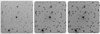 |
Fig. 1 ALFOSC field of view around WASP-12, the brightest star in the center of each image. From left to right: without ED; with ED #1 on; and with ED #2 on, where the ghosts described in Sect. 2.4 are clearly seen around the brightest stars in the field. |
Basic characteristics of the engineered diffusers.
2.4 Efficiency of the diffusers and ghosts
To determine the throughput of the EDs, on December 2, 2018, and on January 20, 2019, we observed two standard star fields found in the Landolt (1992) catalog, namely RU 152 to characterize ED #1 in the U, B, V, R, I filters, and SA98 670 to characterize ED #2 in the U, B, V, R, I and SDSS g&z filters. First, we carried out a set of U, B, V, R, I images to monitor the zero point of ALFOSC, followed by the following sequence of observations for each filter studied: (a) filter only, (b) filter + diffuser, (c) filter only, and (d) filter + diffuser. This resulted in four images per filter. This observing strategy allowed us to isolate the throughput of the EDs, effectively correcting for instrument throughput and CCD quantum efficiency variations as the measurements were taken a few seconds apart. For this exercise, we typically used the same integration time as for the zero-point monitoring.
The bright isolated stars were selected from a zero-point frame and these coordinates were used for the whole sequence. The number of stars analyzed per filter ranged between 14 and 21 for ED #1, and 24 and 37 for ED #2. In all cases fluxes were measured in analog to digital units (ADUs) using the IRAF apphot task, with an aperture of 30 pixels (approximately 5.7 arcseconds). In most cases, the images with and without diffuser have a similar median count, suggesting that the sky was clear and the night photometric. Figure 4 shows the median throughput for ED #1 in the top panel, and for ED #2 in the bottom panel in the U, B, V, R, I and the U, B, g, V, R, I, z sets of filters, respectively. The throughput ratios were computed averaging the flux counts from each set of images for the respective filters.
In the figures it can be seen that ED #1 has a throughput of about 90% in the B filter, peaking at 92% in the R filter. The U filter shows a drop placing the throughput around 80%. The throughput for ED #2 has a similar trend, but with slightly lower values, peaking at 90% in the red. The drop in the U band is caused by the inefficiency of the coating at these wavelengths (see Table 2).
Furthermore, from our test images taken with ED #2, we found a structure around the brightest stars, especially when the count peaks were above ~60% the total dynamic range of the ALFOSC CCD. We call these features ghosts. Figure 5 shows the ghosts near bright stars that were captured using different filters. The two-sided ghost appears to be stronger in bluer wavelengths than in redder ones. When the star is at the center of the field of view, the ghost on the left is stronger than the one on the right. However, this is reversed when the star is close to the edge of the field of view. To produce the figure, the data were overscan subtracted, but not flat field corrected. To estimate the relative intensity between the stellar flux and the ghosts, we measured their respective count levels using IRAF task imexamine. While stellar intensities are given by the counts at the peak of the PSFs, the intensity of the ghosts are estimated averaging a 5 × 5 pixel square near the maximum of the structure, determined from visual inspection. The ratio between the stellar intensity peak and the averaged ghost counts is approximately 196 for U, 296 for B, 550 for V, 1290 for R, 3500 for I, and 290 for g, revealing the increase in its contribution toward bluer wavelengths. The z band seems to show no ghosts. In all cases the ratios are so large that we do not expect – and do not observe – that these features will have any impact in the quality of the photometry.
Technical specifications of the EDs given by the manufacturer, RPC Photonics.
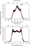 |
Fig. 2 Diffusing pattern of the EDs as a function of unbinned pixels (bottom axis) and arcseconds (top axis). The diffused PSF profiles from ED #1 and ED #2 are shown in theupper and lower panels, respectively. The red line shows the intra-night averaged PSF profile. |
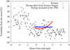 |
Fig. 3 Variability of airmass (red squares), local seeing (black circles), and FWHM of diffuser-assisted science frames (blue diamonds) as a function of time within a single night of observations. The seeing was calculated by the TNG staff, and the diffuser-assisted observations used ED #1 in ALFOSC. |
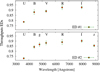 |
Fig. 4 Throughput of ED #1 (top) and ED #2 (bottom). Error bars show the standard deviation of the measured stellar flux ratios. |
3 Observations and data reduction
3.1 Collected data
In Table 3 we summarize the main characteristics of all our science observations.
On the night of August 16, 2018, we observed one primary transit of TrES-3b with ED #1. The host star has a magnitude of R = 11.98(O’Donovan et al. 2007), making it a relatively bright source for the collecting area of the NOT. The transit is fully covered, with about 15 min of out-of-transit data before and after the transit. The night was stable and clear. The data were taken in 1 × 1 binning using a Bessel R filter, centered at 650 ± 130 nm. The overall averaged cadence accounting for readout time was 36 s, while the exposure time was set to 25 s. The night was photometricand with good seeing, slowly and steadily increasing between 0.5 and 1.5 arcseconds throughout the night.
On the night of December 11, 2018, we observed one primary transit of CoRoT-1b using ED #1. The transit coverage was complete, with 45 min and 1 h of out-of-transit data before and after the transit, respectively. The magnitude of the host star is V = 13.6, and its spectral type is G0V (Guenther et al. 2012). We observed the host star and several comparison stars during primary transit in 1 × 1 binning using a Bessel B filter (440 ± 100 nm). To the best of our knowledge, these data correspond to the bluest transit observations of CoRoT-1b carried out to date. Due to the magnitude of the host star, the overall cadence was 180 s. The seeing varied in the night between 0.5 and 2′′, but most of the time it was well below 1′′. The night was photometric throughout.
Finally, on the nights of January 1, 12, and 24, 2019, we observed three secondary eclipses of WASP-12b, the first and third using ED #1 and the second using ED #2. In all cases the secondary eclipses are fully covered, with approximately 20 min to 1 h of out-of-eclipse data before and after the events. Following the given dates, the overall cadences were between 43, 37, and 87 s. All eclipses were observed with the Bessel V filter, with the main goal was to characterize the geometric albedo of the exoplanet (see Sect. 5.3 for further details).
Most relevant parameters describing our observations.
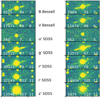 |
Fig. 5 Stellar intensity profiles where the ghosts can be clearly seen. Test images were taken for several different photometricfilters. Left: the brightest star is close to the edge of the field of view. Right: the brightest star is placed at the center of the field of view. The notation “Bessel” corresponds to Bessel filters, and “SDSS” to Sloan filters. |
3.2 Data reduction
The data reduction was carried out by means of our Differential Photometry Pipelines for Optimum Lightcurves, DIP2 OL. The procedure is fully described in von Essen et al. (2018). In brief, the photometric reduction pipeline is based in the IRAF command language, and carries out normal calibration sequences such as bias and dark subtraction and flatfielding, using the task ccdproc. The science frames are then scrutinized for cosmic rays using the IRAF task cosmicrays. Afterward, the calibrated images are aligned using xregister, and counts within several combinations of different apertures and sky rings are computed. The apertures are distributed between 0.5 and 5 times the average stellar PSF FWHM of the night computed directly from the science frames, while the sky rings are between 1 and 3. As the PSFs are diffused, it is worth noting that the seeing we compute is absolutely not representative of the local seeing of the site. For the data detrending (see Sect. 4) DIP2 OL outputs the airmass, the seeing, the (x,y) pixel coordinates of the centroid positions, the background counts determined within the sky rings, and the integrated master flatfield and master dark counts for each aperture, when available. The last three quantities are computed per measured star. Our data reduction finishes converting the time axis given in Julian dates to barycentric Julian dates via the web tool3 presented in Eastman et al. (2010). For this, we use as input values the geographic coordinates of the NOT, along with its altitude above sea level and the celestial coordinates of the stars.
4 Data modeling
4.1 Error determination for the fitting parameters
To determine reliable errors for the parameters fitted in this work, we sample from the posterior-probability distribution using a Markov chain Monte Carlo (MCMC) algorithm. Our MCMC routines are python-based and make use of PyAstronomy4 (based on PyMC, Patil et al. 2010; Jones et al. 2001). To compute our best-fit parameters we iterated 100 000 times per transit and eclipse, and conservatively discarded the first 20% of the samples as burn-in. To investigate the convergence of the chains we first visually inspected them, and then we divided them in three equal parts, computing the best-fit parameters and their errors in each subchain, and verifying consistency among results. In this work, error bars are given at the 1σ level (68.3% credibility intervals).
4.2 Primary transit
As the primary transit model we used the one given by Mandel & Agol (2002). From the transit light curve we can infer the orbital period P, the mid-transit time T0, the planet-to-star radii ratio Rp ∕Rs, the distance between planet and star centers in units of stellar radii a∕Rs, and the orbital inclination i (in degrees). We modeled the stellar limb darkening with a quadratic law, with corresponding limb-darkening coefficients, u1 and u2. These values were taken from Claret & Bloemen (2011) for the filters used, closely matching the effective temperature, metallicity, and surface gravity of each of our observed stars. For the fitting parameters we always considered uniform priors using as starting values those obtained from the literature. The width of the priors was set to ±30 σ′, being σ′ the errors reported by the respective authors.
4.3 Secondary eclipse
As secondary eclipse model we used a scaled version of Mandel & Agol (2002) transit model. In this case, both linear and quadratic limb-darkening coefficients were set to zero. If the transit model is represented by TM(t), then the secondary eclipse model SEM(t) has the following expression:
 (1)
(1)
In the equation, sf denotes the scaling factor. This approach conserves perfectly the transit duration and shape. The eclipse depth is then computed as  , and its error computed from error propagation.
4.4 Datadetrending
Our detrending strategy is fully described in von Essen et al. (2018). In brief, for the detrending model we consider a linear combination of seeing, airmass, centroid positions of the stars involved in the differential photometry, integrated counts over flats and darks on the selected aperture (when available), and integrated sky counts for the selected sky ring. To choose the combination of parameters required to properly detrend the data without over-fitting them, we take into consideration the joint minimization of four statistical indicators: the reduced-χ2 statistic, theBayesian Information Criterion, the standard deviation of the residual light curves enlarged by the number of fitting parameters, and the Cash statistic. During our fitting procedure, at each iteration the detrending coefficients are computed from simple inversion techniques, considering the randomly chosen primary transit or secondary eclipse parameters as fixed. A combined model, consisting of detrending times plus primary transit/secondary eclipses, undergoes the χ2 minimization associated to our MCMC strategy. In consequence, the uncertainties of the detrending coefficients propagate into the uncertainties of the primary transit and secondary eclipse fitting coefficients.
In addition to the detrending strategy produced in von Essen et al. (2018), here we add a further checkup to verify that the detrending does not have a significant impact on the derived fitting parameters. In the case of the secondary eclipses, where the depth is intrinsically low and thus data might suffer most from overfitting, once we determined our best-fit secondary eclipse depth we verified its proper convergence by means of a χ2 map. For the map, we created a grid of secondary eclipse depths within a reasonable range. We assumed that each of these values was the one that reproduces our data best, and we computed the coefficients of the linear combination of the detrending model. With these coefficients, we computed χ2 and plotted its distribution as a function of the eclipse depth. If the detrending process was properly produced and the MCMC chains converged to their absolute minima, the χ2 map should have a unique minimum around the best-fit value. The resulting χ2 maps are given in Sect. 5.
4.5 Noise treatment
To test the extent to which our data are affected by correlated noise (Pont et al. 2006), we followed the approach described in Carter & Winn (2009) and von Essen et al. (2018). After carrying out the MCMC fit, we computed the residual light curves by dividing the photometric data by the best-fit model, and from the residuals we computed the β factor. Briefly, the residuals are divided into M bins of N averaged data points. This average accounts for changes in exposure time that might be needed to compensate for changes in airmass or transparency during the observing runs. If the data show no correlated noise, then the noise contained in the residual light curves should follow the expectation of independent random numbers
![Mathematical equation: \begin{equation*} \hat{\sigma}_N = \sigma N^{-1/2}[M/(M-1)]^{1/2}, \end{equation*}](/articles/aa/full_html/2019/08/aa35312-19/aa35312-19-eq3.png) (2)
(2)
where σ is the standard deviation of the unbinned residual light curve, while σN corresponds to the standard deviation of the data binned with N averaged data points per bin:
 (3)
(3)
Here,  corresponds to the mean value of the residuals per bin (i) and
  is the mean value of the means. If some amount of correlated noise is present in the data, then σN and
  should differ by a factor calledβN. To compute theβ value, we averaged all the βN values obtained from bins that are as large as 0.8, 0.9, 1, 1.1, and 1.2 times the duration of ingress. When β was found to be larger than 1, we enlarged the individual photometric error bars by this factor and carried out the MCMC fitting process again.
5 Results
5.1 TrES-3b
To determine our best-fit parameters from the data collected during the primary transit of TrES-3b, as starting values for the transit parameters, we used the values found in O’Donovan et al. (2007; their Table 3). Since we have only one transit light curve, the orbital period was considered fixed using the value reported in the literature. We then fitted the mid-transit time, the distance between planet and star centers in units of stellar radii, the inclination, and the planet-to-star radii ratio. Our derived results, along with 1σ error bars, are listed in Table 4. Our values are fully consistent with those reported by O’Donovan et al. (2007), with smaller uncertainties. Figure 6 shows the raw data as gray squares, the combined model as a blue continuous lines, the detrended data as black circles, and the best-fit transit model as a red continuous line. The standard deviation of the residual light curve for an exposure time of 25 s is 0.5 parts per thousand (ppt), and the corresponding β value is very close to 1. It is worth noting that this target was also observed by Stefansson et al. (2017) using their own ED with a similar diffusing angle (0.34 versus 0.35°). For their test observations they used the 3.5 m Astrophysical Research Consortium Telescope, located at Apache Point Observatory, USA. Even though their collecting area is significantly larger than that of the NOT, their achieved precision is 0.75 ppt at a 32.5 second cadence. To our knowledge, the only other ground-based transit light curve of TrES-3b more precise than the one reported here can be found in Parviainen et al. (2016). The authors observed TrES-3b with the 10m Gran Telescopio Canarias and the OSIRIS low-resolution spectrograph, achieving in their white light curve a 0.5 ppt scatter for 12 s exposure.
Transit parameters (TPs) for TrES-3b.
5.2 CoRoT-1b
For CoRoT-1b, as initial values for our MCMC fit we used the parameters found in Bean (2009), their Table 1 and 3, which in turn were derived from a global fit of 36 transit light curves taken with the CoRoT space-based telescope, 20 of them taken in long cadence (512 s exposures corresponding to a 0.681 ppt photometric precision) and the remainder taken in CoRoT “short runs” (32 s with a photometric precision of 2.724 ppt; see Baglin et al. 2006, for the definitions of long cadence and short run).
In Table 5 we list our best-fit transit parameters along with the 1σ errors, compared tothe ones reported by the authors. All values are consistent within uncertainties to the ones reported by Bean (2009). Figure 7 shows the detrended transit photometry as black circles, along with our best-fit transit model as a red continuous line. The standard deviation of the residual light curve, for an exposure time of 162 s, is 0.65 ppt. The corresponding β value is close to 1. Considering that our exposure time is three times smaller than the CoRoT long cadence, our derived photometricprecision is significantly superior than CoRoT’s.
As previously mentioned, our data were taken with ED #1 simultaneously with the Bessel B filter. Besides Turner et al. (2016)’s near-UV transit, our derived planet-to-star radii ratio is one of the bluest point characterized in the CoRoT-1b transmissionspectrum. Figure 8 shows its complete transmission spectrum. A nonchromatic planet-star radius ratio results in a χ2 of 15.79 with 11 degrees of freedom (equivalently, a reduced χ2 of 1.43) and a probability P of 0.1. Thus, the current set of observations does not show significant variations in Rp /Rs. CoRot-1bhas an atmospheric pressure scale height of ~700 Km. Models of hot-Jupiter transmission spectra predict variations in Rp ∕Rs in low spectral resolution within approximately ±2 scale heights (Fortney et al. 2010; Schlawin et al. 2014). The mean uncertainty of the existent measurement for Rp ∕Rs, and the uncertainty of the new measurement of this work roughly correspond to this value of two scale heights. In consequence, the data are not precise enough for a detailed transmission model fitting. Nonetheless, the new B-band data point is lower than the mean by ~2.5 scale heights. The optical transmission spectra of many other hot Jupiters show an increase in the Rp ∕Rs values toward short wavelengths of about a few scale heights due to scattering (Sing et al. 2016; Mallonn & Wakeford 2017). Thus, the observations reported here disfavor a typical scattering signature in the transmission spectrum of CoRoT-1b. If confirmed by follow-up observations, it might be indicative of a gray absorption by clouds composed of rather large condensate particles (Wakeford & Sing 2015).
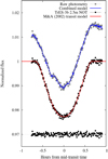 |
Fig. 6 Primary transit photometry for TrES-3b as a function of the hours from the best-fit mid-transit time. From top to bottom: raw photometry (gray squares) along with the combined best-fit model (transit times detrending) (blue solid line). Black circles and error bars correspond to the detrended photometry, and the red continuous line to the best-fit transit model. Residuals are shown below. All quantities are artificially shifted to allow for visual inspection. |
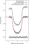 |
Fig. 7 Primary transit photometry of CoRoT-1b as a function of the hours from the best-fit mid-transit time. The figure description is the same as given in Fig. 6. |
5.3 WASP-12b
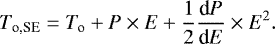
The three eclipses of WASP-12b were fitted independently from each other, using the fitting strategy described in the previous sections. For the scaling factor of the primary transit we allowed both positive (physical) and negative (nonphysical) values. To fit the scaling factor we considered uniform priors corresponding to a reasonable secondary eclipse depth of ±3 ppt. For thetransit parameters we adopted the values recently reported by Maciejewski et al. (2018), particularly for an orbital period that allows for the observed orbital decay. The mid-eclipse times for our observed secondary eclipses, To,SE, were computed from a quadratic ephemeris:
 (4)
(4)
Here, E corresponds to the epoch of the observation with respect to the mid-transit time of reference To. The values of To, P, and  can be found in Table 6, along with other relevant transit parameters fully adopted in this work. In Table 7 we list the best-fit secondary eclipse depths for the three dates, along with other information that reflects the quality of our data and fit. The left panels of Fig. 9 shows our resulting secondary eclipse light curves for the mentioned nights, and the right panels show our χ2 maps for each of them, compared to the MCMC best-fit values and errors at a 2σ level. In all cases, the detrending parameters that were always favored were the x,y centroid positions of the stars and the airmass. The first set of parameters does not come as a surprise as the telescope was passing very close to the zenith where the stability of the tracking is not optimal. Because of this, a ~20-min gap is clearly seen during the first and second nights. This data gap is mostly produced by our 5σ clipping algorithm that takes place during the construction of the raw light curves as these data points naturally have large photometricuncertainties. Originally, some sparse data points were left within the gap, but we found that including them in the fitting procedure made the number of detrending parameters reach their maximum to account for this noise. In consequence, to minimize the number of detrending components we discarded the few points left inside the gap, and carried out our usual fittingprocedure with the minimum possible detrending components. Finally, the extinction of light crossing our atmosphere is an effect that is inherent in the diffusers, and thus is found in our detrending components as well.
WASP-12 is a triple-star system with a separation of only 1′′ between the primarycomponent and its low-mass companions (Bechter et al. 2014). In the V band, the flux contribution of the two companions amounts to about 0.9% (Crossfield et al. 2012) and is fully included in our photometric apertures. The measured eclipse depth of Table 7 are diluted by this amount and need to be corrected upward by 0.9%. However, we report the uncorrected, diluted values because the correction is one order of magnitude smaller than the given uncertainties.
The depth of the first eclipse measurement deviates by about 5σ from the depth of the second and third event. The latter are in agreement at the 2σ level. Observations of the secondary eclipse of the same target in an overlapping wavelength regime have been published by Bell et al. (2017). The V band corresponds to their two reddest wavelength bins, which resulted in a depth of 0.06 ± 0.1 ppt when averaged. This value is in good agreement with the result of our second event; however, our first and third event results deviate by 6σ and 2.5σ, respectively.
Potentially, systematic noise might mimic the deep ingress and egress features of our first eclipse event. However, we find no abnormal behavior in any instrumental parameters at this time. Also, the very close match of the ingress/egress timings to the predicted times makes an instrumental or systematic origin of these features less likely. The literature offers additional hints for a time-variability of the eclipse depth of WASP-12b. Observations obtained in the Sloan z′ band at 0.9 μm by López-Morales et al. (2010) and Föhring et al. (2013) disagreed at the 2.4σ level. Very recently, Hooton et al. (2019) measured two eclipses of WASP-12b in the Sloan i′ band that differed by ~3σ. For another very hot Jupiter, WASP-19b, discrepant results have been published by Burton et al. (2012) and Lendl et al. (2013) that might potentially be explained by variability in time.
We assume that the origin of the different eclipse depths in this work is a variability in time, and we want to briefly discuss the potential sources. The depth of a secondary eclipse is the sum of light reflected by the planet toward the observer and thermally emitted light from the planet. We use Eqs. (4) and (5) of Alonso (2018) for a rough estimation of the potential time variability of these two components. The thermal radiation of planet and host star is approximated by blackbody radiation. For the involved stellar and planetary parameters, we adopt the values of Collins et al. (2017). If we keep the thermal component fixed to a planetary blackbody radiation of 2900 K (Stevenson et al. 2014), our secondary eclipse values can be explained by a range of the geometric albedo from zero to ~0.75. Reflective clouds formed by large-size condensates might cause a geometric albedo of up to 0.4 (Sudarsky et al. 2000), and we are not aware of any physical mechanisms causing a higher albedo in the dayside atmosphere of WASP-12b, thus a geometric albedo of 0.75 appears unlikely.
If the variability of the eclipse depth is purely explained by an increase in thermal radiation, a planetary temperature of about 4000 K is needed. However, an increase in planetary temperature of 1000 K would result in even more pronounced depth variations at near-IR wavelengths. The rough agreement of all existent near-IR secondary eclipse data of WASP-12b, taken at different epochs, to a blackbody temperature of about 3000 K (e.g., Cowan et al. 2012; Stevenson et al. 2014) makes a significant time variability of the photospheric temperature unlikely.
Could both components act together to produce the large eclipse depth of our first measurement? If we assume the temporary formation of a reflective cloud deck causing a geometric albedo of 0.4, our simple estimation results in an additional requirement of an increased blackbody temperature to ~3600 K. However, a spontaneous cloud formation would intuitively be associated with a decrease in temperature instead of an increase; therefore, it is unclear under what circumstances the reflective light component and the thermal light component can be enhanced at the same time. Additionally, we note that on the dayside of WASP-12b no cloud formation is expected because the very high temperatures do not allow for particle condensation (Wakeford et al. 2017).
The WASP-12 system is known to contain material eroded and blown away from the planetary atmosphere by the extreme stellar irradiation (Fossati et al. 2013). We can only speculate whether the variable eclipse depth might not be caused by the planetary dayside atmosphere, but by an inhomogeneous flow of escaping material. This material might form temporary clumps near the planet, which scatter a fraction of the starlight toward the observer. In this scenario, the deep secondary eclipse would be caused by an occultation of the escaping material rather than by the occultation of the planet.
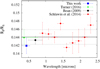 |
Fig. 8 Transmission spectrum of CoRoT-1b, with planet-to-star radii ratio obtained from this work (blue square), Turner et al. (2016; green triangle), Bean (2009; black circle), and Schlawin et al. (2014; red diamonds). Horizontal continuous and dashed lines indicate the mean and ± the standard deviation of the data points, respectively. |
Description of our observations of WASP-12b.
6 Conclusions
In this workwe present the characterization of two brand new engineered diffusers (EDs) mounted at the 2.5-m Nordic Optical Telescope. The diffusers have two slightly different diffusing angles, spreading the light of the stars differently over the CCD. They can be placed in two different filter wheels and can work simultaneously with several photometric filters placed on a third wheel. To characterize the stability and reliability of the EDs, we observed two photometric standard stars. We found the throughput of the diffusers to be superior to 90% in the visible and for redder wavelengths, dropping down to ~75% in the ultraviolet, as expected from their construction and design. Both the core and the wings of the diffused stellar images are quite stable as observations evolve, without significant changes that correlate with seeing or airmass. Furthermore, we observed three exoplanetary systems, namely TrES-3b, CoRoT-1b, and WASP-12b. While the first two were observed during one primary transit each, the third was followed-up during three secondary eclipse events. Since the EDs can be combined with regular photometric filters, our science frames were taken using the Bessel B, V, and R filters. The achieved photometric precision of 0.5 ppt for a 25-s exposure in TrES-3b, 0.65 ppt for 162 s for CoRoT-1b, and between 0.52 and 0.59 ppt for less than one-minute cadence for WASP-12b clearly shows the power of engineered diffusers to achieve high-precision photometricdata. In addition, we presented a new planet-to-star radii ratio for CoRoT-1b, to our knowledge the bluest data point taken to date, and we observed a significant variability in the eclipse depth of WASP-12b, as previously pointed out by other authors using other optical wavelengths. Within our collected data we observed a deviation within eclipse depths of about 5σ. From previous observations in a similar wavelength range, our first and third eclipse depths deviate by 6σ and 2.5σ. The reasons for this variability are purely speculative.
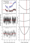 |
Fig. 9 Left: secondary eclipse data of WASP-12b obtained with the NOT and the EDs turned on. Black circles and error bars correspond to the photometric data. The red continuous line shows the best-fit secondary eclipse, in ppt. For the most prominent eclipse we show raw photometry (gray squares), along with the combined best-fit model (transit times detrending) (blue solid line). Right: χ2 maps for different scaling factors. The thick black line corresponds to the χ2 values obtained for different eclipse depths. The red vertical line indicates the minimization of χ2, and the black solid vertical line, along with the two dashed lines, indicate the best-fit MCMC results and a ±2σ contour. |
Acknowledgements
C.v.E. acknowledges funding for the Stellar Astrophysics Centre provided by The Danish National Research Foundation (Grant DNRF106), and support from the European Social Fund via the Lithuanian Science Council grant No. 09.3.3-LMT-K-712-01-0103. This work made use of PyAstronomy5. The data presented here were obtained with ALFOSC, which is provided by the Instituto de Astrofisica de Andalucia (IAA) under a joint agreement with the University of Copenhagen and NOTSA. G.K.S. acknowledges support by NASA Headquarters under the NASA Earth and Space Science Fellowship Program - Grant NNX16AO28H. J.F. and S.D. acknowledge funding from the German Research Foundation (DFG) through grant DR 281/30-1 and DR 281/32-1.
References
- Alonso, R. 2018, Characterization of Exoplanets: Secondary Eclipses (Basel, Switzerland: Springer International Publishing AG), 40 [Google Scholar]
- Baglin, A., Auvergne, M., Boisnard, L., et al. 2006, in COSPAR Meeting, 36th COSPAR Scientific Assembly, 36 [Google Scholar]
- Baglin, A., Auvergne, M., Barge, P., et al. 2009, in Transiting Planets, eds. F. Pont, D. Sasselov, & M. J. Holman, IAU Symp., 253, 71 [NASA ADS] [CrossRef] [Google Scholar]
- Bakos, G., Noyes, R. W., Kovács, G., et al. 2004, PASP, 116, 266 [NASA ADS] [CrossRef] [Google Scholar]
- Barge, P., Baglin, A., Auvergne, M., et al. 2008, A&A, 482, L17 [NASA ADS] [CrossRef] [EDP Sciences] [Google Scholar]
- Bean, J. L. 2009, A&A, 506, 369 [NASA ADS] [CrossRef] [EDP Sciences] [Google Scholar]
- Bechter, E. B., Crepp, J. R., Ngo, H., et al. 2014, ApJ, 788, 2 [NASA ADS] [CrossRef] [Google Scholar]
- Bell, T. J., Nikolov, N., Cowan, N. B., et al. 2017, ApJ, 847, L2 [NASA ADS] [CrossRef] [Google Scholar]
- Borucki, W. J., Koch, D., Basri, G., et al. 2010, Science, 327, 977 [NASA ADS] [CrossRef] [PubMed] [Google Scholar]
- Burton, J. R., Watson, C. A., Littlefair, S. P., et al. 2012, ApJS, 201, 36 [NASA ADS] [CrossRef] [Google Scholar]
- Carter, J. A., & Winn, J. N. 2009, ApJ, 704, 51 [NASA ADS] [CrossRef] [Google Scholar]
- Claret, A., & Bloemen, S. 2011, A&A, 529, A75 [NASA ADS] [CrossRef] [EDP Sciences] [Google Scholar]
- Collins, K. A., Kielkopf, J. F., & Stassun, K. G. 2017, AJ, 153, 78 [NASA ADS] [CrossRef] [Google Scholar]
- Cowan, N. B., Machalek, P., Croll, B., et al. 2012, ApJ, 747, 82 [NASA ADS] [CrossRef] [Google Scholar]
- Crossfield, I. J. M., Barman, T., Hansen, B. M. S., Tanaka, I., & Kodama, T. 2012, ApJ, 760, 140 [NASA ADS] [CrossRef] [Google Scholar]
- Deeg, H. J., Gillon, M., Shporer, A., et al. 2009, A&A, 506, 343 [NASA ADS] [CrossRef] [EDP Sciences] [Google Scholar]
- Eastman, J., Siverd, R., & Gaudi, B. S. 2010, PASP, 122, 935 [NASA ADS] [CrossRef] [Google Scholar]
- Föhring, D., Dhillon, V. S., Madhusudhan, N., et al. 2013, MNRAS, 435, 2268 [NASA ADS] [CrossRef] [Google Scholar]
- Fortney, J. J., Shabram, M., Showman, A. P., et al. 2010, ApJ, 709, 1396 [NASA ADS] [CrossRef] [Google Scholar]
- Fossati, L., Ayres, T. R., Haswell, C. A., et al. 2013, ApJ, 766, L20 [NASA ADS] [CrossRef] [Google Scholar]
- Freudenthal, J., von Essen, C., Dreizler, S., et al. 2018, A&A, 618, A41 [NASA ADS] [CrossRef] [EDP Sciences] [Google Scholar]
- Guenther, E. W., Gandolfi, D., Sebastian, D., et al. 2012, A&A, 543, A125 [NASA ADS] [CrossRef] [EDP Sciences] [Google Scholar]
- Halverson, S., Mahadevan, S., Ramsey, L., et al. 2014, in Ground-based and Airborne Instrumentation for Astronomy V, SPIE Conf. Ser., 9147, 91477Z [Google Scholar]
- Hebb, L., Collier-Cameron, A., Loeillet, B., et al. 2009, ApJ, 693, 1920 [NASA ADS] [CrossRef] [Google Scholar]
- Hooton, M. J., de Mooij, E. J. W., Watson, C. A., et al. 2019, MNRAS, 486, 2397 [NASA ADS] [CrossRef] [Google Scholar]
- Howell, S. B., Everett, M. E., Tonry, J. L., Pickles, A., & Dain, C. 2003, PASP, 115, 1340 [NASA ADS] [CrossRef] [Google Scholar]
- Howell, S. B., Sobeck, C., Haas, M., et al. 2014, PASP, 126, 398 [NASA ADS] [CrossRef] [Google Scholar]
- Johnson, J. A., Winn, J. N., Cabrera, N. E., & Carter, J. A. 2009, ApJ, 692, L100 [NASA ADS] [CrossRef] [Google Scholar]
- Jones, E., Oliphant, T., Peterson, P., et al. 2001, SciPy: Open source scientific tools for Python, http://www.scipy.org [Google Scholar]
- Kempton, E. M.-R., Bean, J. L., Louie, D. R., et al. 2018, PASP, 130, 114401 [NASA ADS] [CrossRef] [Google Scholar]
- Kjeldsen, H., & Frandsen, S. 1992, PASP, 104, 413 [NASA ADS] [CrossRef] [Google Scholar]
- Lafrenière, D., Doyon, R., Nadeau, D., et al. 2007, ApJ, 661, 1208 [NASA ADS] [CrossRef] [Google Scholar]
- Landolt, A. U. 1992, AJ, 104, 340 [NASA ADS] [CrossRef] [Google Scholar]
- Lendl, M., Gillon, M., Queloz, D., et al. 2013, A&A, 552, A2 [NASA ADS] [CrossRef] [EDP Sciences] [Google Scholar]
- López-Morales, M., Coughlin, J. L., Sing, D. K., et al. 2010, ApJ, 716, L36 [NASA ADS] [CrossRef] [Google Scholar]
- Maciejewski, G., Fernández, M., Aceituno, F., et al. 2018, Acta Astron., 68, 371 [NASA ADS] [Google Scholar]
- Mallonn, M., & Wakeford, H. R. 2017, Astron. Nachr., 338, 773 [NASA ADS] [CrossRef] [Google Scholar]
- Mandel, K., & Agol, E. 2002, ApJ, 580, L171 [NASA ADS] [CrossRef] [Google Scholar]
- O’Donovan, F. T., Charbonneau, D., Bakos, G. Á., et al. 2007, ApJ, 663, L37 [NASA ADS] [CrossRef] [Google Scholar]
- Parviainen, H., Pallé, E., Nortmann, L., et al. 2016, A&A, 585, A114 [NASA ADS] [CrossRef] [EDP Sciences] [Google Scholar]
- Patil, A., Huard, D., & Fonnesbeck, C. J. 2010, J. Stat. Softw., 35, 1 [CrossRef] [EDP Sciences] [Google Scholar]
- Pepper, J., Pogge, R. W., DePoy, D. L., et al. 2007, PASP, 119, 923 [NASA ADS] [CrossRef] [Google Scholar]
- Pollacco, D. L., Skillen, I., Collier Cameron, A., et al. 2006, PASP, 118, 1407 [NASA ADS] [CrossRef] [Google Scholar]
- Pont, F., Zucker, S., & Queloz, D. 2006, MNRAS, 373, 231 [NASA ADS] [CrossRef] [Google Scholar]
- Ricker, G. R., Winn, J. N., Vanderspek, R., et al. 2015, J. Astron. Telesc. Instrum. Syst., 1, 014003 [NASA ADS] [CrossRef] [Google Scholar]
- Schlawin, E., Zhao, M., Teske, J. K., & Herter, T. 2014, ApJ, 783, 5 [NASA ADS] [CrossRef] [Google Scholar]
- Sing, D. K., Fortney, J. J., Nikolov, N., et al. 2016, Nature, 529, 59 [NASA ADS] [CrossRef] [Google Scholar]
- Smith, A. M. S., Collier Cameron, A., Christian, D. J., et al. 2006, MNRAS, 373, 1151 [NASA ADS] [CrossRef] [Google Scholar]
- Southworth, J., Hinse, T. C., Jørgensen, U. G., et al. 2009, MNRAS, 396, 1023 [NASA ADS] [CrossRef] [Google Scholar]
- Stefansson, G., Mahadevan, S., Hebb, L., et al. 2017, ApJ, 848, 9 [NASA ADS] [CrossRef] [EDP Sciences] [Google Scholar]
- Stefansson, G., Li, Y., Mahadevan, S., et al. 2018a, AJ, 156, 266 [NASA ADS] [CrossRef] [Google Scholar]
- Stefansson, G., Mahadevan, S., Wisniewski, J., et al. 2018b, in Ground-based and Airborne Instrumentation for Astronomy VII, SPIE Conf. Ser., 10702, 1070250 [Google Scholar]
- Stevenson, K. B., Bean, J. L., Madhusudhan, N., & Harrington, J. 2014, ApJ, 791, 36 [NASA ADS] [CrossRef] [Google Scholar]
- Sudarsky, D., Burrows, A., & Pinto, P. 2000, ApJ, 538, 885 [NASA ADS] [CrossRef] [Google Scholar]
- Tingley, B. 2004, A&A, 425, 1125 [NASA ADS] [CrossRef] [EDP Sciences] [Google Scholar]
- Tonry, J., Burke, B. E., & Schechter, P. L. 1997, PASP, 109, 1154 [NASA ADS] [CrossRef] [Google Scholar]
- Turner, J. D., Pearson, K. A., Biddle, L. I., et al. 2016, MNRAS, 459, 789 [NASA ADS] [CrossRef] [Google Scholar]
- von Essen, C., Cellone, S., Mallonn, M., Tingley, B., & Marcussen, M. 2016, ArXiv e-prints [arXiv:1607.03680] [Google Scholar]
- von Essen, C., Ofir, A., Dreizler, S., et al. 2018, A&A, 615, A79 [NASA ADS] [CrossRef] [EDP Sciences] [Google Scholar]
- Wakeford, H. R., & Sing, D. K. 2015, A&A, 573, A122 [NASA ADS] [CrossRef] [EDP Sciences] [Google Scholar]
- Wakeford, H. R., Visscher, C., Lewis, N. K., et al. 2017, MNRAS, 464, 4247 [NASA ADS] [CrossRef] [Google Scholar]
All Tables
All Figures
|
Fig. 1 ALFOSC field of view around WASP-12, the brightest star in the center of each image. From left to right: without ED; with ED #1 on; and with ED #2 on, where the ghosts described in Sect. 2.4 are clearly seen around the brightest stars in the field. |
| In the text | |
|
Fig. 2 Diffusing pattern of the EDs as a function of unbinned pixels (bottom axis) and arcseconds (top axis). The diffused PSF profiles from ED #1 and ED #2 are shown in theupper and lower panels, respectively. The red line shows the intra-night averaged PSF profile. |
| In the text | |
|
Fig. 3 Variability of airmass (red squares), local seeing (black circles), and FWHM of diffuser-assisted science frames (blue diamonds) as a function of time within a single night of observations. The seeing was calculated by the TNG staff, and the diffuser-assisted observations used ED #1 in ALFOSC. |
| In the text | |
|
Fig. 4 Throughput of ED #1 (top) and ED #2 (bottom). Error bars show the standard deviation of the measured stellar flux ratios. |
| In the text | |
|
Fig. 5 Stellar intensity profiles where the ghosts can be clearly seen. Test images were taken for several different photometricfilters. Left: the brightest star is close to the edge of the field of view. Right: the brightest star is placed at the center of the field of view. The notation “Bessel” corresponds to Bessel filters, and “SDSS” to Sloan filters. |
| In the text | |
|
Fig. 6 Primary transit photometry for TrES-3b as a function of the hours from the best-fit mid-transit time. From top to bottom: raw photometry (gray squares) along with the combined best-fit model (transit times detrending) (blue solid line). Black circles and error bars correspond to the detrended photometry, and the red continuous line to the best-fit transit model. Residuals are shown below. All quantities are artificially shifted to allow for visual inspection. |
| In the text | |
|
Fig. 7 Primary transit photometry of CoRoT-1b as a function of the hours from the best-fit mid-transit time. The figure description is the same as given in Fig. 6. |
| In the text | |
|
Fig. 8 Transmission spectrum of CoRoT-1b, with planet-to-star radii ratio obtained from this work (blue square), Turner et al. (2016; green triangle), Bean (2009; black circle), and Schlawin et al. (2014; red diamonds). Horizontal continuous and dashed lines indicate the mean and ± the standard deviation of the data points, respectively. |
| In the text | |
|
Fig. 9 Left: secondary eclipse data of WASP-12b obtained with the NOT and the EDs turned on. Black circles and error bars correspond to the photometric data. The red continuous line shows the best-fit secondary eclipse, in ppt. For the most prominent eclipse we show raw photometry (gray squares), along with the combined best-fit model (transit times detrending) (blue solid line). Right: χ2 maps for different scaling factors. The thick black line corresponds to the χ2 values obtained for different eclipse depths. The red vertical line indicates the minimization of χ2, and the black solid vertical line, along with the two dashed lines, indicate the best-fit MCMC results and a ±2σ contour. |
| In the text | |
Current usage metrics show cumulative count of Article Views (full-text article views including HTML views, PDF and ePub downloads, according to the available data) and Abstracts Views on Vision4Press platform.
Data correspond to usage on the plateform after 2015. The current usage metrics is available 48-96 hours after online publication and is updated daily on week days.
Initial download of the metrics may take a while.