| Issue |
A&A
Volume 628, August 2019
|
|
|---|---|---|
| Article Number | A35 | |
| Number of page(s) | 15 | |
| Section | Celestial mechanics and astrometry | |
| DOI | https://doi.org/10.1051/0004-6361/201935304 | |
| Published online | 01 August 2019 | |
New light on the Gaia DR2 parallax zero-point: influence of the asteroseismic approach, in and beyond the Kepler field
1
School of Physics and Astronomy, University of Birmingham, Edgbaston, Birmingham B15 2TT, UK
e-mail: This email address is being protected from spambots. You need JavaScript enabled to view it.
2
Stellar Astrophysics Centre, Department of Physics and Astronomy, Aarhus University, Ny Munkegade 120, 8000 Aarhus C, Denmark
3
LESIA, Observatoire de Paris, PSL Research University, CNRS, Sorbonne Université, Université Paris Diderot, 92195 Meudon, France
4
GEPI, Observatoire de Paris, PSL Research University, CNRS, 92195 Meudon, France
5
Leiden Observatory, Leiden University, Niels Bohrweg 2, 2333 CA Leiden, The Netherlands
6
Research School of Astronomy and Astrophysics, Mount Stromlo Observatory, The Australian National University, ACT 2611, Australia
7
ARC Centre of Excellence for All Sky Astrophysics in 3 Dimensions (ASTRO 3D), Australia
8
Osservatorio Astronomico di Padova, INAF, Vicolo dell’Osservatorio 5, 35122 Padova, Italy
9
Institut de Ciències del Cosmos, Universitat de Barcelona (IEEC-UB), Martí i Franquès 1, 08028 Barcelona, Spain
Received:
19
February
2019
Accepted:
27
May
2019
Abstract
The importance of studying the Gaia DR2 parallax zero-point by external means was underlined by the articles that accompanied the release, and initiated by several works making use of Cepheids, eclipsing binaries, and asteroseismology. Despite a very efficient elimination of basic-angle variations, a small fluctuation remains and shows up as a small offset in the Gaia DR2 parallaxes. By combining astrometric, asteroseismic, spectroscopic, and photometric constraints, we undertake a new analysis of the Gaia parallax offset for nearly 3000 red-giant branch (RGB) and 2200 red clump (RC) stars observed by Kepler, as well as about 500 and 700 red giants (all either in the RGB or RC phase) selected by the K2 Galactic Archaeology Program in campaigns 3 and 6. Engaging in a thorough comparison of the astrometric and asteroseismic parallaxes, we are able to highlight the influence of the asteroseismic method, and measure parallax offsets in the Kepler field that are compatible with independent estimates from literature and open clusters. Moreover, adding the K2 fields to our investigation allows us to retrieve a clear illustration of the positional dependence of the zero-point, in general agreement with the information provided by quasars. Lastly, we initiate a two-step methodology to make progress in the simultaneous calibration of the asteroseismic scaling relations and of the Gaia DR2 parallax offset, which will greatly benefit from the gain in precision with the third data release of Gaia.
Key words: asteroseismology / astrometry / parallaxes / stars: low-mass
© ESO 2019
1. Introduction
Masses and radii of solar-like oscillating stars can be estimated from the global asteroseismic observables that characterise their oscillation spectra, namely the average large frequency separation (⟨Δν⟩) and the frequency corresponding to the maximum observed oscillation power (νmax). The large frequency spacing is predicted by theory to approximately scale as the square root of the mean density of the star (see e.g. Vandakurov 1967; Tassoul 1980),
 (1)
(1)
where M and R are the stellar mass and radius, respectively. The maximum power frequency follows a proportional relation with the acoustic cut-off frequency to good approximation, and can provide a direct measure of the surface gravity (g) when the effective temperature (Teff) is known (see e.g. Brown et al. 1991; Kjeldsen & Bedding 1995; Belkacem et al. 2011):
 (2)
(2)
Equations (1) and (2) imply that if ⟨Δν⟩ and νmax are available, together with an independent estimate of Teff, a “direct” estimation of the stellar mass and radius is possible. This direct method is particularly attractive because in principle it provides estimates that are independent of stellar models. Alternatively, one may also use ⟨Δν⟩ and νmax as inputs to a grid-based estimation of the stellar properties, matching the observations to stellar evolutionary tracks – either using the scalings at face value or stellar pulsation calculations to obtain ⟨Δν⟩ (e.g. Stello et al. 2009; Basu et al. 2010; Gai et al. 2011; Rodrigues et al. 2017). Whether it be with the direct or the grid-based approach, a plethora of studies have compared asteroseismic measurements of radii (or distances) with independent ones, such as clusters (Miglio 2012; Miglio et al. 2016; Stello et al. 2016; Handberg et al. 2017), interferometry (Huber et al. 2012), eclipsing binaries (Gaulme et al. 2016; Brogaard et al. 2016, 2018), and astrometry (Silva Aguirre et al. 2012; De Ridder et al. 2016; Davies et al. 2017; Huber et al. 2017; Sahlholdt et al. 2018; Zinn et al. 2019). All these works indicated that stellar radius estimates from asteroseismology are accurate to within a few per cent.
On the astrometric side and before the Gaia data, the asteroseismic distances of stars (which arise from the combination of seismic constraints with effective temperature and apparent photometric magnitudes) in the solar neighbourhood had only been compared a posteriori with HIPPARCOS values. These comparisons were limited due to the HIPPARCOS uncertainties being large for most of the Kepler and CoRoT targets (Miglio 2012; Silva Aguirre et al. 2012; Lagarde et al. 2015). The announcement of the first Gaia data release opened the gates to the Gaia era (Gaia Collaboration 2016a,b). Parallaxes and proper motions were available for the two million brightest sources in Gaia DR1, as part of the Tycho-Gaia Astrometric Solution (TGAS; Lindegren et al. 2016). As the TGAS parallaxes considerably improved the HIPPARCOS values, a new comparison between astrometric and asteroseismic parallaxes was appropriate. Some works took the path of the model-independent method, that is using asteroseismic distances based on the use of the raw scaling relations. Using assumptions about the luminosity of the red clump, Davies et al. (2017) found the TGAS sample to overestimate the distance, with a median parallax offset of −0.1 mas. For 2200 Kepler stars, from the main sequence to the red-giant branch, Huber et al. (2017) obtained a qualitative agreement, especially if they adopted a hotter effective temperature scale for dwarfs and subgiants. The latter suggestion was corroborated by Sahlholdt et al. (2018). In contrast, De Ridder et al. (2016) used seismic modelling methods to analyse two samples of stars observed by Kepler: 22 nearby dwarfs and subgiants showing an excellent overall correspondence; and 938 red giants for which the TGAS parallaxes were significantly smaller than the seismic ones. Given the different seismic approaches and the various outcomes, the situation as regards to the Gaia DR1 parallax offset and as probed by asteroseismology was left unclear.
The second data release of Gaia was published on April 25 2018 (Gaia Collaboration 2018), based on the data collected during the first 22 months of the nominal mission lifetime (Gaia Collaboration 2016b). Gaia DR2 represents a major advance with respect to the first intermediate Gaia data release, containing parallaxes and proper motions for over 1.3 billion sources. Unlike the TGAS, the Gaia DR2 astrometric solution does not incorporate any information from HIPPARCOS and Tycho-2. However, with less than two years of observations and preliminary calibrations, a few weaknesses in the quality of the astrometric data remain, and were identified by Arenou et al. (2018) and Lindegren et al. (2018). Among these caveats, the latter study underlined the importance of investigating the parallax zero-point by external means, and did so through the use of quasars. In this matter, quasars are a quasi-ideal means given the negligibly small parallaxes, large number, and availability over most of the celestial sphere. A global zero-point of about −30 μas was found by Lindegren et al. (2018), in the sense that Gaia parallaxes are too small, with variations of the order of several tens of μas, depending on a given combination of magnitude, colour, and position. Quasars have their own specific properties, such as their faintness and blue colour, which should be kept in mind when interpreting these results. For this reason, a direct correction of individual parallaxes from the global parallax zero-point is discouraged (Arenou et al. 2018).
In this context, several works have confirmed the existence of a parallax offset by independent means. In a study of 50 Cepheids, Riess et al. (2018) suggest a zero-point offset of −46 ± 13 μas. Stassun & Torres (2018) present evidence of a systematic offset of about −82 ± 33 μas with 89 eclipsing binaries. And, finally, Zinn et al. (2019) infer a systematic error of −52.8 ± 2.4 (statistical) ±1 (systematic) μas for 3500 first-ascent giants in the Kepler field, using asteroseismic and spectroscopic constraints from Pinsonneault et al. (2018) who used model-predicted corrections to the ⟨Δν⟩ scaling relation. Very little difference was found with 2500 red-clump stars: −50.2 ± 2.5 (statistical) ±1 (systematic) μas, which is expected from the astrometric point of view since Gaia, unlike seismology, does not make any distinction between shell-hydrogen and core-helium burning stars.
These various outcomes demonstrate the need to independently solve the parallax zero-point within the framework of an analysis having its own specificities, meaning magnitude, colour, and spatial distributions. In the case of asteroseismology, the findings of a comparison with Gaia DR2 cannot be dissociated from the seismic method employed. With this in mind, we engage in a thorough investigation of the Gaia DR2 parallax offset in the Kepler field by taking an incremental approach, starting with the scaling relations taken at face value and gradually working towards a Bayesian estimation of stellar properties using a grid of models (Sect. 4). Also, looking at the broader picture and considering two fields of the re-purposed Kepler mission, K2, allows us to investigate the positional dependence of the zero-point (Sect. 5). Lastly, Gaia DR2 offers scope for development in the calibration of the scaling relations, and we initiate a two-step methodology allowing us to constrain the Gaia DR2 offset at the same time (Sect. 6).
2. Observational framework
2.1. Description of the datasets
One part of our sample consists of red-giant stars observed by Kepler and with available APOGEE spectra (APOKASC collaboration; Abolfathi et al. 2018). From the initial list of stars, we selected those that are classified as RGBs and RCs (including secondary clump stars) using the method by Elsworth et al. (2017). We considered the global asteroseismic parameters ⟨Δν⟩ and νmax. We used the frequency of maximum oscillation power, νmax, from Mosser et al. (2011). Two methods for providing relevant estimates of ⟨Δν⟩ are discussed in Sect. 2.2. We also made use of the spectroscopically measured effective temperature Teff, surface gravity log g (calibrated against asteroseismic surface gravities), and of constraints on the photospheric chemical composition [Fe/H] and [α/Fe] from SDSS DR14, as determined by the APOGEE Pipeline (Abolfathi et al. 2018). This leads us to 3159 RGB stars and 2361 RC stars in the Kepler field.
Our Kepler subsample is then complemented with red giants selected by the K2 Galactic Archaeology Program (GAP; Howell et al. 2014; Stello et al. 2015, 2017) in campaigns 3 (south Galactic cap) and 6 (north Galactic cap), which have SkyMapper photometric constraints (Casagrande et al. 2019). We made use of the asteroseismic analysis method from Mosser et al. (2011) for the vast majority, and from Elsworth et al. (2017) for a very small fraction of stars (∼5%). Details about additional tests of the reliability of seismic results can be found in Rendle et al. (2019). For Teff and [Fe/H], we used the photometric estimates originating from the SkyMapper survey (Casagrande et al. 2019), while log g is obtained from asteroseismically-derived estimates. This K2 subsample falls into two parts: 505 and 723 red giants in C3 and C6, respectively.
For the full sample, stellar masses and extinctions are inferred using the Bayesian tool PARAM (Rodrigues et al. 2014, 2017). Asteroseismic constraints ⟨Δν⟩ and νmax are included in the modelling procedure in a self-consistent manner, whereby ⟨Δν⟩ is calculated from a linear fitting of the individual radial-mode frequencies of the models in the grid. PARAM also requires photometry and uses its own set of bolometric corrections (described at length in Girardi et al. 2002) to estimate distances and extinctions. For comparison purposes, we also calculated extinctions via the Green et al. (2015) dust map and the Rayleigh-Jeans Colour Excess (RJCE) method (Majewski et al. 2011). The bolometric corrections were derived using the code written by Casagrande & VandenBerg (2014, 2018a,b), taking Teff, log g and [Fe/H] as input parameters. The second data release of Gaia (Gaia Collaboration 2016b, 2018) then provided us with astrometric and photometric constraints: parallaxes (using the external parallax uncertainty as described by Lindegren et al. in their overview of Gaia DR2 astrometry1, and made available by the Gaia team at the GEPI, Observatoire de Paris2), G-band magnitudes (corrected following Casagrande & VandenBerg 2018a, i.e. Gcorr = 0.0505 + 0.9966 G), and GBP − GRP colour indices. The 2MASS (Skrutskie et al. 2006) K-band photometry is used as well.
2.2. Consistency in the definition of ⟨Δν⟩
For the Kepler field (Sect. 4), we explored different seismic methods, which have to be matched with a consistent definition of ⟨Δν⟩. To use ⟨Δν⟩ in the scaling relations, one would want to adopt a measure which is as close as possible to the asymptotic limit (on which the scaling is based). This implies, for example, correcting for acoustic glitches, which are regions of sharp sound-speed variation in the stellar interior related to a rapid change in the chemical composition, the ionisation of major chemical elements, or the transition from radiative to convective energy transport (see e.g. Miglio et al. 2010; Vrard et al. 2015). In this case, the ⟨Δν⟩ measured by Mosser et al. (2011) is appropriate since their method mitigates the perturbation on ⟨Δν⟩ due to glitches. On the other hand, one could abandon scalings and use ⟨Δν⟩ from models that can, for example, be based on individual frequencies as in PARAM, which also takes into account departures from homology (regarding the assumption of scaling with density, i.e. Eq. (1)). Then, it is more adequate to combine PARAM with ⟨Δν⟩ estimates from individual radial-mode frequencies. While the latter are currently available only for a small subset (697 RGB and 783 RC stars), following the approach presented in Davies et al. (2016), we noticed a qualitative agreement with ⟨Δν⟩ from Yu et al. (2018), which are also derived from the frequencies. On the contrary, the ⟨Δν⟩ as determined by Mosser et al. (2011) has a different definition that is closer to the analytical asymptotic relation. Its value for RGB stars is systematically larger by ∼1% compared to the one from individual mode frequencies, as shown in Fig. 1. Meanwhile, there is no specific trend in the difference between the two ⟨Δν⟩ estimates for RC stars.
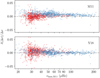 |
Fig. 1. Relative difference in ⟨Δν⟩, δ(Δν)/Δν = (Δνother − ΔνD16)/ΔνD16, between individual frequencies following Davies et al. (2016, D16) and another method, as a function of νmax as estimated by Mosser et al. (2011). The comparison is done with Mosser et al. (2011, M11; top) and Yu et al. (2018, Y18; bottom). RGB and RC stars are in blue and red, respectively. Here, Δν is used, instead of ⟨Δν⟩, to simplify the notation. |
Therefore, in Sect. 4.1, we use raw scaling relations in combination with ⟨Δν⟩ from Mosser et al. (2011). Then, in Sects. 4.2 and 4.3 where theoretically-motivated corrections to the ⟨Δν⟩ scaling are used, we adopt ⟨Δν⟩ from Yu et al. (2018) instead.
3. Detailed objectives
In order to simplify the statistical analysis of our results, we formulated the problem in the astrometric data space, meaning parallax space. Significant biases can arise from the inversion of parallaxes into distances and from sample truncation, such as the removal of negative parallaxes and/or parallaxes with a relative error above a given threshold (Luri et al. 2018). Thus, in the current investigation, we avoided doing any of these. On the other hand, it is quite reasonable to invert asteroseismic distances to obtain parallaxes because their uncertainties are typically lower than a few per cent (see, e.g. Rodrigues et al. 2014).
If one wishes to express the parallax as a function of the apparent and intrinsic luminosity of a star, this can be done using the Stefan–Boltzmann law, as follows:
 (3)
(3)
where Rbb is the radius of the black body of effective temperature Teff, that is the photospheric radius, and cλ = 10−0.2 (mλ+BCλ+5−Aλ−Mbol, ⊙). mλ, BCλ, and Aλ are the magnitude, bolometric correction, and extinction in a given band λ, respectively. We adopt Mbol, ⊙ = 4.75 for the Sun’s bolometric magnitude. Thereafter, we will resort to the 2MASS K-band magnitude properties (mK, BCK, and AK), whenever we need to estimate the coefficient cλ.
3.1. Asteroseismic parallax
Engaging in such a parallax comparison requires a way to express the seismic information in terms of parallax, to be compared to the Gaia astrometric measurements. Seismic parallaxes are also based on the Stefan-Boltzmann law. Going back to the foundations of ensemble asteroseismology, seismic scaling relations provide relevant estimates of the stellar masses and radii. From Eqs. (1) and (2), their expressions are as follows:
 (4)
(4)
 (5)
(5)
involving both global asteroseismic observables ⟨Δν⟩ and νmax, and Teff. The solar references are taken as ⟨Δν⟩⊙ = 135 μHz, νmax, ⊙ = 3090 μHz, and Teff, ⊙ = 5777 K. It is assumed here that the seismic radius, R, and the black-body radius, Rbb, are the same. Finally, using Eqs. (3) and (5), the seismic parallax ensuing from the scaling relations can be written as
 (6)
(6)
The seismic scaling relations have been widely used, even though it is known that they are not yet precisely calibrated. Testing their validity has become a very active topic in asteroseismology, and has been addressed in several ways. It may take the form of a comparison between asteroseismic radii and independent measurements of stellar radii (e.g. Huber et al. 2012, 2017; Gaulme et al. 2016; Miglio et al. 2016). An alternative approach consists in validating the relation between the average large frequency separation and the stellar mean density from model calculations (Ulrich 1986). The asymptotic approximation for acoustic oscillation modes tells us that ⟨Δν⟩ is directly related to the sound travel-time in the stellar interior, and therefore depends on the stellar structure (Tassoul 1980). As mentioned in Sect. 1, Eq. (1) is approximate and assumes that stars, in general, are homologous to the Sun and that the measured ⟨Δν⟩ corresponds to ⟨Δν⟩ in the asymptotic limit; in practice, that is not the case (for further details see e.g. Belkacem et al. 2013). The sound speed in their interior (hence the total acoustic travel-time) does not simply and only scale with mass and radius. In particular, whether a red-giant star is burning hydrogen in a shell or helium in a core, its internal temperature (hence sound speed) distribution will be different. This led several authors to quantify any deviation from the ⟨Δν⟩ scaling relation these differences could cause (e.g. White et al. 2011; Miglio et al. 2012; Belkacem 2012; Guggenberger et al. 2016; Sharma et al. 2016; Rodrigues et al. 2017). Stellar evolution calculations show that the deviation varies by a few per cent with mass, chemical composition, and evolutionary state. That is why the seismic parallax can also be estimated from the large separation determined with grid-based modelling, meaning statistical methods taking into account stellar theory predictions (e.g. allowed combinations of mass, radius, effective temperature, and metallicity) as well as other kinds of prior information (e.g. duration of evolutionary phases, star formation rate, and initial mass function). In particular, the Bayesian tool PARAM uses ⟨Δν⟩, νmax, Teff, log g, [Fe/H], [α/Fe] (when available), and photometric measurements to derive probability density functions for fundamental stellar parameters, including distances (Rodrigues et al. 2014, 2017).
The asteroseismic results thus depend on the method employed. This aspect is explored in more detail in Sect. 4, where three distinct seismic methods are tested (with the appropriate ⟨Δν⟩, as discussed in Sect. 2.2): the raw scaling relations, a relative correction to the ⟨Δν⟩ scaling between RGB and RC stars, and a model-grid-based Bayesian approach defining ⟨Δν⟩ from individual frequencies. Furthermore, in Sect. 6, we combine asteroseismic and astrometric data to simultaneously calibrate the scaling relations and the Gaia zero-point.
3.2. Method
Our study is based on the analysis of the absolute rather than the relative difference between Gaia and seismic parallaxes: Δϖ = ϖGaia − ϖseismo. This is for two reasons: first, the global zero-point offset in Gaia parallaxes is absolute (Lindegren et al. 2018); second, working in terms of relative difference can amplify trends, for example due to offsets having a greater impact on small parallaxes.
We explored the trends of the measured offset (Δϖ) for a set of stellar parameters: the Gaia parallax ϖGaia, the G-band magnitude, the frequency of maximum oscillation νmax, the GBP − GRP colour index, the mass inferred from PARAM (MPARAM), and the metallicity [Fe/H]. Each of these relations is described with a linear fit obtained through a RANSAC algorithm (Fischler & Bolles 1981). The fitting parameters’ uncertainties are estimated by making N = 1000 realisations of the set of parameters analysed with RANSAC, where a normally distributed noise is added using the observed uncertainties on Δϖ and the different stellar parameters. Because the fitting parameters are strongly dependent on the range of values covered by the independent variable X (the stellar parameter in question), the fits are expressed in the following form:  . αX is the slope, βX is the intercept from which
  was subtracted, and
  is the mean value of the stellar parameter X (Table 1).
Values of  (mean value of the stellar parameter X) for RGB (top) and RC stars (bottom).
As part of the analysis, some summary statistics can be given. We first consider the median parallax difference  and the associated uncertainty
  . Then, we also give the weighted average parallax difference
  and its uncertainty
  , which are defined as follows:
 (7)
(7)
 (8)
(8)
The latter corresponds to the weighted standard deviation, which gives a measure of the spread and also takes the individual (formal) uncertainties in Δϖ into account. Finally, the ratio  is given, where
  is the uncertainty of the weighted mean estimated from the formal uncertainties on Δϖ. This ratio allows one to assess how well the formal fitting uncertainties reflect the scatter in the data. If the Δϖ scatter is dominated by random errors and the formal uncertainties reflect the true observational uncertainties, then z is close to unity. In the following, unless stated otherwise, the weighted average parallax difference estimator will be used for the offsets quoted in the text.
4. Analysis of the Kepler field
In this section, we focus on the comparison between Gaia DR2 and asteroseismology for red giants in the Kepler field. We take advantage of the classification method from Elsworth et al. (2017) that is based on the structure of the dipole-mode oscillations of mixed character. This method distinguishes between shell-hydrogen burning stars on the red-giant branch and core-helium burning stars in the red clump (including secondary clump stars, as well). From the asteroseismic perspective, three different approaches are employed in order to emphasise the influence of the seismic method on the measured parallax zero-point.
4.1. Raw scaling relations
We start with the raw scaling relations, to which no correction has been applied. The seismic parallax is directly estimated from Eq. (6), using ⟨Δν⟩ from Mosser et al. (2011). The comparison with Gaia parallaxes is shown in Figs. 2 and 3 for RGB and RC stars, respectively. At first sight, we observe a strong dependence of the RGB parallax difference with ϖGaia, that is, as the latter increases, Δϖ significantly increases as well (Fig. 2, top-left panel). Such a trend also appears for RC stars, but to a much lesser extent. In fact, the parallax zero-point is expected to show variations depending on position, magnitude, and colour (Lindegren et al. 2018) but not on parallax, unless we consider stars with the same intrinsic luminosity (e.g. RC stars; see Fig. 3). In such a case, the dependence on apparent magnitude would manifest itself as a dependence on parallax. In addition, for core-helium burning stars, one can see that there is a cut-off at low astrometric parallaxes (ϖGaia < 350 μas; Fig. 3, top-left panel). This is most likely related to the selection in magnitude in Kepler (see e.g. Farmer et al. 2013), which translates into a limit on distance. Gaia parallaxes, having larger uncertainties compared to their asteroseismic counterparts, can lead to distances greater than this limit and, when represented on the x-axis, create a horizontal structure (adding to the vertical structure caused by the scatter of the parallax difference) as observed. Conversely, if we had the seismic parallax on the x-axis instead, such a structure would disappear and the slope would become flatter. Still, we note that these trends might either come from the seismic parallax or from the correlation between the parallax difference and the Gaia parallax. Having a deeper look at the summary statistics, there seems to be a considerable difference in the measured offset: that of RGB stars reaches up to −8 μas, compared to RC stars displaying an average value of −36 μas. On their own, these results could be interpreted as a minimal difference between astrometric and asteroseismic measurements for stars along the RGB, but there remains the issue of the apparent trends of Δϖ with parallax.
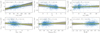 |
Fig. 2. Parallax difference ϖGaia − ϖseismo for RGB stars, with the asteroseismic parallax derived from raw scaling relations, as a function of ϖGaia, G, νmax, GBP − GRP, MPARAM, and [Fe/H]. The distribution of the N realisations of the RANSAC algorithm is indicated by the grey-shaded region and the yellow line displays the average linear fit, for which the relation is given at the top of each subplot. The values of |

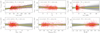 |
Fig. 3. Same as Fig. 2 but for RC stars. The values of |

To clarify this situation, in Fig. 4 we show the relation between the seismic and Gaia parallaxes, separately for RGB and RC stars. While the latter display a relation nearly parallel to the 1:1 line, RGB stars show a slope of 1.028 ± 0.007, which is significantly different from 1 and is not solely due to a correlation effect. Because all sources are treated as single stars in Gaia DR2, the results for resolved binaries may sometimes be spurious due to confusion of the components (Lindegren et al. 2018). The Re-normalised Unit Weight Error (RUWE) is recommended as a goodness-of-fit indicator for Gaia DR2 astrometry (see the technical note GAIA-C3-TN-LU-LL-124-01 available from the DPAC Public Documents page3). It is computed from the following quantities:
-
χ2 = astrometric_chi2_al;
-
N= astrometric_n_good_obs_al;
-
G;
-
and GBP − GRP.
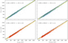 |
Fig. 4. ϖGaia as a function of ϖscaling (left) and ϖPARAM (right), for RGB (top) and RC (bottom) stars. The yellow line indicates the linear fit, averaged over N realisations, for which the relation is given at the top of each subplot. The black dashed line indicates the 1:1 relation. |
Figure 5 shows the distribution of the RUWE for stars in the Kepler field, including both RGB and RC evolutionary phases (their distinction does not affect the shape of the distribution). Because there seems to be a breakpoint around RUWE = 1.2 between the expected distribution for well-behaved solutions and the long tail towards higher values, we adopt RUWE ≤ 1.2 as a criterion for “acceptable” solutions. By imposing this condition, the scatter is reduced, but the slope appearing in Fig. 4 is still present and the offset remains unchanged. Therefore, this steep slope could potentially be a symptom of biases in the seismic scaling relations. To a good approximation, the changes in the slope due to changes in Teff, or modifications in the scaling relations, can be obtained as linear perturbations of Eq. (6). The question of their calibration using Gaia data is addressed in Sect. 6. In addition, the similar distributions of the RUWE for RGB and RC stars also point in favour of the fact that the quality of Gaia parallaxes is not responsible for the different behaviour of these stars in Figs. 2 and 3.
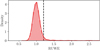 |
Fig. 5. Re-normalised Unit Weight Error (RUWE) distribution for Kepler RGB and RC stars. The vertical dashed line indicates the threshold adopted: RUWE ≤ 1.2. |
A fairly strong trend also appears for the parallax difference as a function of the G-band magnitude, especially in the case of RGB stars (Fig. 2, top-middle panel). Within Gaia itself, observations are acquired in different instrumental configurations and need to be calibrated separately depending on, for example, the window class and the gate activation (for further details see e.g. Riello et al. 2018). In the range of magnitudes covered by red-giant stars, several changes occur:
-
at G = 11.5, the BP/RP (blue photometer/red photometer) window class switches from 2D to 1D;
-
at G = 12, there is the transition between gated (to avoid saturation affecting bright sources) and un-gated observations;
-
at G = 13, the AF (Astrometric Field) window class changes from 2D to 1D.
In order to separate the different effects, we divide the RGB and RC samples in bins of G as follows: G ≤ 11.5, G ∈ [11.5, 12], G ∈ [12, 13], and G > 13. Doing so results in an offset decreasing from 16 to −21 μas between the lowest and the highest bins for RGB stars, and from −28 to −44 μas for RC stars. We remark that the trend of the offset with increasing magnitude is negative in both cases, but stronger for RGB stars than for RC stars (see top-middle panels in Figs. 2 and 3), which might again indicate a problem regarding the raw scaling relations. Δϖ does not seem to exhibit any noteworthy relation with the other stellar parameters. Hence, they will not be shown throughout the rest of the paper, apart from νmax, which is an important asteroseismic indicator of the evolutionary stages.
Despite the above, using the raw scaling relations has the considerable advantage of giving us the agility and flexibility to have a direct test of potential systematic effects. In any case, we later show that a lot of the departures of the slopes from unity can be removed by using grid-based modelling (Sect. 4.3). Here, we explore the influence that other non-seismic inputs, meaning the effective temperature scale and the extinctions, may have on the comparison. Teff appears explicitly in Eq. (6), but also implicitly through the bolometric correction contained in the coefficient cλ, the definition of which is given in Sect. 3. The combination of these two factors leads to an increase (or decrease) of both the ϖscaling–ϖGaia slope coefficient and the offset with increasing (or decreasing) Teff: a ±100 K shift results in a ±10−15 μas variation in the parallax difference. Reducing the effective temperature by 100 K is almost enough to obtain a slope of ∼1, but not to have an offset in agreement with the red clump. On the other hand, setting the extinctions to zero or doubling their values barely affects the parallax difference, at the order of ±6 μas at the most. As a check, in Fig. 6, we compare our extinction values with those derived by Green et al. (2015) (Bayestar15) and from the RJCE method (Majewski et al. 2011), to see if they are consistent with each other. For the most part, the differences are within the ±0.02 level, with a larger scatter on the RJCE side. The typical (median) uncertainties on the extinctions are 0.007, 0.002, and 0.025 for PARAM, Bayestar15, and RJCE, respectively. At low extinction values (AK < 0.025), Bayestar15’s extinctions are systematically larger, introducing a diagonal shape in the distribution. This is most likely a truncation effect caused by the fact that Bayestar15 only provides strictly non-negative extinction estimates, while PARAM derives both positive and negative AK (Rodrigues et al. 2014). Such differences are not expected to significantly affect our comparison, as already implied by the above tests given that the parallax offsets measured with these extinctions only differ by approximately ±2 μas. This is also partly due to the fact that we are using an infrared passband, which reduces the impact of reddening.
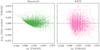 |
Fig. 6. Absolute difference in AK between PARAM and another method, as a function of PARAM’s extinctions. The comparison is made with the Green et al. (2015) map (left) and the RJCE method (right). |
4.2. Corrected ⟨Δν⟩ scaling relation
From theoretical models, one expects that deviations from the ⟨Δν⟩ scaling relation depend on mass, chemical composition, and evolutionary state, as discussed in Sect. 3.1. Nevertheless, at fixed mass and metallicity (e.g. for a cluster), one can derive a relative correction to the scaling between RGB and RC stars, modifying Eq. (1) as follows: ⟨Δν⟩′ = 𝒞⟨Δν⟩⟨Δν⟩, where 𝒞⟨Δν⟩ is a correction factor. This has been done for the open cluster NGC 6791: Miglio et al. (2012) compared asteroseismic and photometric radii, while Sharma et al. (2016) estimated 𝒞⟨Δν⟩ along each stellar track of a grid of models (see also Rodrigues et al. 2017). Both found a relative correction of ∼2.7% between the two evolutionary stages, 𝒞⟨Δν⟩ being larger and closer to unity for RC stars. The value of 2.7% corresponds to the low-mass end (M ∼ 1.1 M⊙). The relative correction would be of the order of 2.5% for 1.2–1.3 M⊙ stars.
Hence, as a first-order approximation, we applied this correction to our RGB sample: namely, for each star, we reduced ⟨Δν⟩ from the scaling relation by 2.7%. As this correction is based on a definition of ⟨Δν⟩ from individual frequencies, it makes sense to use ⟨Δν⟩ from Yu et al. (2018) to ensure consistency. Figure 7 shows how the inclusion of this correction from modelling affects the comparison for stars along the RGB. After applying the relative correction, the estimated offset became −35 μas, which is much closer to what was obtained with RC stars (Fig. 3), possibly indicating the relevance of the correction. However, even if the relations of Δϖ with the Gaia parallax and the G-band magnitude seem flatter, the ϖrel–ϖGaia relation now displays a slope of 0.984 ± 0.007. This is most likely due to the application of an average correction initially derived for NGC 6791, and not quite suitable for the wide range of masses and metallicities covered by the sample. Finally, to help quantify the effect of this correction, we also estimated the slope and the parallax offset using ⟨Δν⟩ from Mosser et al. (2011), as in the previous section, and obtained 0.974 and −43 μas. Thus, the dominant effect here is that of the correction, rather than the change of ⟨Δν⟩.
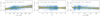 |
Fig. 7. Same as Fig. 2 but with the asteroseismic parallax derived from scaling relations with a 2.7% correction factor applied to the ⟨Δν⟩ scaling. The summary statistics are: |
4.3. ⟨Δν⟩ from individual frequencies: grid-modelling
With their Bayesian tool PARAM, Rodrigues et al. (2017) replaced the ⟨Δν⟩ scaling relation with an average large frequency definition stemming from a linear fitting of the individual radial-mode frequencies computed along the evolutionary tracks of the grid. Similarly, and as stated above, we use ⟨Δν⟩ as estimated by Yu et al. (2018) for consistency with the ⟨Δν⟩ definition adopted in the models in PARAM. At this time, this approach has yielded masses and radii that show no systematic deviations to within a few per cent of independent estimates (see e.g. Miglio et al. 2016; Handberg et al. 2017; Rodrigues et al. 2017; Brogaard et al. 2018, who partially revisited the work by Gaulme et al. 2016). This method requires the use of a grid of models covering the complete relevant range of masses, ages, and metallicities. It is worth emphasising that the physical inputs of the models play a crucial role in the determination of stellar parameters via a Bayesian grid-based method. There is no absolute set of stellar models, and a few changes in their ingredients may also affect the outcome of an investigation such as ours. For details about the models considered here, we refer the reader to Rodrigues et al. (2017), with the exception that here we include element diffusion.
The comparison of the Gaia parallaxes with the seismic ones estimated with PARAM appears in Fig. 8 for RGB stars, and Fig. 9 for RC stars. Both evolutionary phases have a flattened relation with ϖGaia such that they now display similar slopes. In the RGB sample, the ϖPARAM–ϖGaia relation has a slope nearly equal to unity: 0.998 ± 0.003 and that of the RC stars is largely unchanged (see Fig. 4). These effects bring the parallax zero-points very close: −52 and −48 μas for RGB and RC stars, respectively. The trends with G are also relatively flat, resulting in small fluctuations as we move from low to high G magnitudes: from −58 to −51 μas for stars on the RGB, and from −46 to −52 μas in the clump. These findings are reassuring in the sense that, if we were to find a trend with parallax or an evolutionary-state dependent offset, the issue would be down to seismology. Since we do not observe such effects, it seems relevant to use PARAM with appropriate constraints to derive asteroseismic parallaxes. If we were to combine PARAM with ⟨Δν⟩ estimates from Mosser et al. (2011) instead, the RGB and RC offsets would become −62 and −46 μas, respectively. This would introduce a significant relative difference in the parallax zero-point between RGB and RC stars, which is neither due to the presence of secondary clump stars, nor to the different νmax ranges covered by RGB and RC stars. Furthermore, the effect on the slopes is a decrease for RGB stars (0.986) and a very mild increase for RC stars (1.002). Again, these findings highlight the importance of ensuring consistency in the ⟨Δν⟩ definition between observations and models.
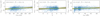 |
Fig. 8. Same as Fig. 2 but with the asteroseismic parallax derived from PARAM (Rodrigues et al. 2017). The summary statistics are: |
What follows below aims at quantifying how sensitive the findings with PARAM are on additional systematic biases such as changes in the Teff and [Fe/H] scales, and the use of different model grids. We tested that a ±100 K shift in Teff affects Δϖ by ±3 μas for RGB stars, but this left the results largely unchanged for RC stars. It is not surprising that the order of magnitude of these variations is lower compared to when we used the scaling relations at face value (±10–15 μas). The grid of models restricts the possible range of Teff values for a star with a given mass and metallicity, even more so when dealing with the very localised core-helium burning stars. Then, a ±0.1 dex shift in [Fe/H] affects Δϖ by ∓4 and ∓2 μas for RGB and RC stars, respectively. Finally, when considering models computed without diffusion (described in Rodrigues et al. 2017), the parallax zero-point slightly increases for RGB stars (Δϖ∼ − 57 μas) and decreases for RC stars (Δϖ∼ − 41 μas), enhancing the discrepancy between the two evolutionary phases. Grids of models computed with and without diffusion differ, for example in terms of the mixing-length parameter, and of the initial helium and heavy-elements mass fractions obtained during the calibration of a solar model. Because of these combined effects, it is complex to interpret the respective impacts on RGB and RC stars. Since models with diffusion are in better agreement with, for instance, the helium abundance estimated in the open cluster NGC 6791 (Brogaard et al. 2012) and constraints on the Sun from helioseismology (Christensen-Dalsgaard 2002), they are our preferred choice for the current study. However, we stress that, at this level of precision, uncertainties related to stellar models are non-negligible (see Miglio et al., in prep.).
As a summary, Fig. 10 shows how the ϖseismo–ϖGaia slopes and parallax offsets (weighted average parallax difference) evolve as we move from the scaling relations taken at face value to grid-based modelling. This illustrates the convergence of RGB and RC stars both in terms of slope and offset when using PARAM.
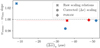 |
Fig. 10. Slope of the various ϖseismo–ϖGaia relations as a function of the weighted average parallax difference for RGB (blue) and RC (red) stars. The results using raw scaling relations (crosses; Sect. 4.1), a corrected ⟨Δν⟩ scaling relation (circles; Sect. 4.2), and PARAM (diamonds; Sect. 4.3) are shown. For RC stars, the line is extended to lower offset values for a better visualisation of how the slope compares with RGB stars when using scaling relations at face value. |
4.4. External validation with open clusters
We performed an external validation of our findings by using independent measurements for the open clusters NGC 6791 and NGC 6819, both in the Kepler field. We adopted the distances given by eclipsing binaries: dNGC 6791 = 4.01 ± 0.14 kpc (Brogaard et al. 2011) and dNGC 6819 = 2.52 ± 0.15 kpc (Handberg et al. 2017). The comparison with Gaia DR2 parallax measurements (Cantat-Gaudin et al. 2018) gives offsets of −60.6 ± 8.9 μas and −40.4 ± 23.6 μas for the former and the latter, respectively. This is reassuring as it is in line with the results obtained with PARAM.
4.5. Influence of spatial covariances
As discussed by Lindegren et al. (2018; see also Arenou et al. 2018), spatial correlations are present in the astrometry, leading to small-scale, systematic errors. The latter have a size comparable to that of the focal plane of Gaia, that is ∼0.7°. In comparison, the Kepler field, with an approximate radius of 7°, is very large. The uncertainty on the inferred parallax offset may be largely underestimated, unless one takes these spatial correlations into account. For this reason, we performed a few tests in order to quantify how the various quantities derived in this work (average parallax difference and slope of the linear fits) and their uncertainties would be affected by the presence of spatial covariances. To be as representative as possible, in terms of spatial and distance distributions, we chose to work with our Kepler sample.
We first considered the seismic parallaxes estimated with PARAM as the “true” parallaxes (ϖtrue). This is an arbitrary choice and, thereafter, ϖtrue has to be viewed as a synthetic set of true parallaxes, completely independent from seismology. From there, we computed synthetic seismic and astrometric parallaxes. The former were calculated using the observed uncertainties on PARAM parallaxes (σϖseismo):
 (9)
(9)
where  is a normal distribution with mean zero and variance
  . Then, two sets of astrometric parallaxes are simulated, using the observed uncertainties on Gaia parallaxes (σϖGaia):
 (10)
(10)
 (11)
(11)
where 𝒪Gaia = − 50 μas represents the Gaia parallax zero-point and is set arbitrarily following our findings (Sect. 4.3), and 𝒩(𝒪Gaia, 𝒮) is a multivariate normal distribution with mean 𝒪Gaia and covariance matrix 𝒮. These two parallaxes contain the same random error component ( ), but different systematic error components.
  (Eq. (10)) has a systematic error that is simply equal to the Gaia zero-point; while
  (Eq. (11)) has a systematic error centred on 𝒪Gaia but also accounts for spatial correlations between the sources.
The spatially-correlated errors are assumed to be independent from the random errors, and the corresponding covariance matrix can be written as:
![Mathematical equation: $$ \begin{aligned} \mathcal{S} = E[(\varpi _{i}-\mathcal{O} _{ Gaia})(\varpi _{j}-\mathcal{O} _{ Gaia})] = {\left\{ \begin{array}{ll} V_\varpi (0)&\mathrm if\ i=j \\ V_\varpi (\theta _{ij})&\mathrm if\ i\ne j \end{array}\right.}, \end{aligned} $$](/articles/aa/full_html/2019/08/aa35304-19/aa35304-19-eq39.gif) (12)
(12)
where Vϖ(θ) is the spatial covariance function, which solely depends on the angular distance between sources i and j (θij). Lindegren et al. (2018) suggested
 (13)
(13)
as the spatial correlation function for the systematic parallax errors. To capture the variance at the smallest scales (see Fig. 14 of Lindegren et al. 2018), an additional exponential term can be added:
 (14)
(14)
where the number 1565 μas2 is chosen to get a total Vϖ(0) of 1850 μas2, appearing in the overview of Gaia DR2 astrometry by Lindegren et al4. This value was obtained for quasars, with faint magnitudes (G ≥ 13); for brighter magnitudes (Cepheids), there are indications that a total Vϖ(0) of 440 μas2 would be required instead. However, owing to the uncertainty regarding the exact value that would be suitable for our sample, we preferred to be conservative by using Eq. (14). Lastly, we also tried the description of spatial covariances following Zinn et al. (2019), namely:
 (15)
(15)
As the term 𝒩(𝒪Gaia, 𝒮) in Eq. (11) is subject to important variations between different simulations, we drew Nsims = 1000 realisations of  in order to obtain statistically significant results. Furthermore, because it is computationally expensive to calculate the covariance matrix for a large number of sources, we randomly selected 60% of the RGB and RC samples beforehand. This allowed us to calculate the median parallax difference between the astrometric and seismic synthetic values, as well as its uncertainty. Whether spatial covariances are included or not, we obtain a similar offset (very close to the parallax zero-point applied (𝒪Gaia = −50 μas)) for both RGB and RC stars. The difference becomes apparent when one looks at the uncertainty of the median offset. Without spatial correlations, we find an uncertainty of approximately 1 μas, which is compatible with our results. However, when spatial correlations are included, the uncertainty increases up to ∼14 μas using Eqs. (13) and (14), and it is slightly lower with Eq. (15) (∼10 μas). A similar threshold on the uncertainty of the parallax offset, due to spatial covariances, was recently found by Hall et al. (2019), who used hierarchical Bayesian modelling and assumptions about the red clump to compare Gaia and asteroseismic parallaxes in the Kepler field. Then, studying the relation between the simulated seismic and Gaia parallaxes (in a similar way as in Fig. 4), we find that, regardless of the spatial covariance function applied, the value and uncertainty of the slope parameter are barely affected. This is reassuring since it means that the slopes we obtained in Sects. 4.1–4.3 are significant, and that the argument whereby PARAM displays a slope closer to unity compared to the raw scaling relations is still valid.
5. Positional dependence of the parallax zero-point
This section aims at highlighting how the position constitutes one of the sources of the variations in the Gaia DR2 parallax zero-point. After measuring the offset in the Kepler field, we undertake a similar analysis for two of the K2 Campaign fields: C3 and C6, corresponding to the south and north Galactic caps respectively (Howell et al. 2014). A difference lies in the fact that there is no distinction between the RGB and the RC evolutionary stages here. In the following, we are concerned with the results given by raw scaling relations and PARAM, using the method developed by Mosser et al. (2011) for ⟨Δν⟩ for both approaches as there is no ⟨Δν⟩ available following the approach by Yu et al. (2018). After that, we also analyse the information given by quasars regarding the three fields considered in our investigation.
5.1. K2 fields: C3 and C6
The comparison of parallaxes using the raw scalings with parallaxes from Gaia DR2 is displayed in Fig. 11, and the measured offsets are of the order of 25 ± 4 and 9 ± 3 μas for C3 and C6, respectively. Both have a ϖscaling–ϖGaia relation with a slope substantially different from unity, that is 1.049 ± 0.020 for C3 and 1.071 ± 0.017 for C6. Further, Teff shifts of ± 100 K affect the parallax difference by ±10−15 μas, as is the case for Kepler.
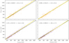 |
Fig. 11. ϖGaia as a function of ϖscaling (left) and ϖPARAM (right) for red giants in the K2 Campaign fields C3 (top) and C6 (bottom). The yellow line displays the linear fit, averaged over N realisations, for which the relation is given at the top of each subplot. The black dashed line indicates the 1:1 relation. The summary statistics are: |
For PARAM, the outcome of the comparison is also illustrated in Fig. 11. C3 displays a parallax difference close to zero (Δϖ≃ − 6 ± 4 μas), while C6 shows a value of about −17 ± 2 μas. In the case of C3, the trend with parallax is entirely suppressed: the slope is equal to 0.999 ± 0.016. It is also reduced for C6, but a fairly steep slope of 1.034 ± 0.009 remains. In absolute terms, these offsets are much lower compared to the Kepler field even though we are dealing with red-giant stars, in both cases either in the RGB or the RC phase. Thus, in the position-magnitude-colour dependence of the parallax zero-point, the position prevails in the current analysis. To test whether these differences are caused by the inhomogeneity in the effective temperatures and metallicities in use between the Kepler and K2 samples, Casagrande et al. (2019) checked the reliability of their photometric metallicities against APOGEE DR14 and found an offset of −0.01 dex with an rms of 0.25 dex, that is [Fe/H] from SkyMapper are lower. Teff from SkyMapper agree with APOGEE DR14 within few tens of K and a typical rms of 100 K. These small deviations should not affect our findings. Also, we compared the extinctions from PARAM that were adopted in this work to those from SkyMapper, which are used to determine Teff and [Fe/H], and find that they are consistent with each other, with differences in AK only at the level of ±0.01. Finally, we investigated the potential origin of the differing slopes between C3 and C6 by considering the different parallax distributions (with respect to each other, and also to the Kepler field); the decreased quality of the K2 seismic data compared to Kepler (Howell et al. 2014); and the use of ⟨Δν⟩ from Mosser et al. (2011) (instead of Yu et al. 2018, as for Kepler). Nevertheless, the interplay between these different elements as well as the limited number of stars in the K2 samples prevent us from drawing any firm conclusion with regards to the slopes. As for the offsets, the effect of such differences seems to be at the level of ∼ ± 7 μas at most. In addition, the fairly good agreement between SkyMapper and APOGEE does not exclude the possibility that the photometric Teff and [Fe/H] may be influenced differently in different fields (e.g. C3 and C6) by external factors such as, for instance, the extinction.
A further point we would like to raise concerns the apparently larger scatter in the K2 fields. In that respect, we identify the order of magnitude of the Gaia and seismic (PARAM) parallax uncertainties (Fig. 12). The asteroseismic uncertainties are slightly larger in the case of K2. This can mainly be explained by the fact that the original mission, Kepler, continuously monitored stars for four years, whereas each campaign of K2 is limited to a duration of approximately 80 days (Howell et al. 2014). Despite this, photometric systematics in the K2 data leading to, for instance, spurious frequencies are now well understood, and the pipelines used to produce light curves have been developed over time to remove or mitigate these effects. As a result, we do not expect the global seismic parameters to show any significant bias due to the K2 artefacts (see also Hekker et al. 2012, and the Kepler and K2 Science Center website5). Nonetheless, the astrometric uncertainties are also substantially larger for K2, almost doubled compared to Kepler. A possible reason for this would be that the regions around the ecliptic plane (such as C3 and C6) are observed less frequently, as a result of the Gaia scanning law, and also under less favourable scanning geometry, with the scan angles not distributed evenly (Gaia Collaboration 2016b). To test this hypothesis, we use the quantity visibility_periods_used: the number of visibility periods, that is a group of observations separated from other groups by a gap of at least four days, used in the astrometric solution. This way, we can assess if a source is astrometrically well-observed. This variable exhibits significantly higher values for Kepler, ranging from 12 to 17. The number of visibility periods for K2 are lower or equal to ten, indicating that the parallaxes could be more vulnerable to errors. The predicted uncertainty contrast between the Kepler and K2 fields is about a factor6 of 1.6, which is indeed consistent with the location of the histogram peaks in the top panel of Fig. 12.
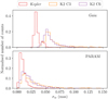 |
Fig. 12. Distribution of parallax uncertainties in Gaia DR2 (top) and in PARAM (bottom) for the Kepler (red), C3 (orange), and C6 (purple) fields. |
5.2. Quasars and colour-magnitude diagram
Lindegren et al. (2018) investigated the parallax offset using quasars, and obtained a global zero-point of about −30 μas. It is no surprise that this value differs from the ones we obtain in the current work. Indeed, this parallax offset depends on magnitude and colour, in addition to position: quasars are generally blue-coloured with faint magnitudes. Red giants are substantially different objects, hence the importance of solving the parallax zero-point independently. We investigated the information provided by quasars to estimate the parallax zero-point in the different fields considered here (see Fig. 13). To this end, we selected quasars within a given radius around the central coordinates of each field and computed the weighted average parallax (following Eq. (8)). The variation of this quantity with radius is shown in Fig. 14. This allows us to assess its sensitivity on the size of the region considered. The mean offsets associated to the size of the fields (r ∼ 7°) are −24 ± 8, 3 ± 9, and −12 ± 7 μas for Kepler, C3, and C6, respectively. It should be kept in mind, however, that spatial covariances in the parallax errors (Sect. 4.5) prevent one from drawing strong conclusions regarding the offsets, especially at the smallest scales. The main purpose of Fig. 14 is to illustrate these trends. Despite exhibiting different values, the pattern whereby the Gaia parallax offset is lowest for C3 and highest for Kepler, in keeping with our results, is potentially reproduced.
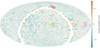 |
Fig. 13. Sky map in ecliptic coordinates of median parallaxes for the full quasar sample, showing large-scale variations of the parallax zero-point. The Kepler (red), C3 (orange), and C6 (purple) fields are displayed. Median values are calculated in cells of 3.7 × 3.7 deg2. |
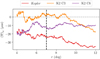 |
Fig. 14. Weighted average parallax of quasars selected within a given radius around the central coordinates of the Kepler (red), C3 (orange), and C6 (purple) fields. The black dashed line indicates the average radius of the fields. |
For illustrative purposes, we show in Fig. 15 two colour-magnitude diagrams (CMDs) for the entire Kepler field: one where the absolute magnitude is calculated without applying a shift in the Gaia parallax, another where we use the zero-point measured with PARAM (∼ − 50 μas for both RGB and RC stars) to “correct” the parallaxes. In addition, owing to the near-zero offset in C3, the latter is also displayed for comparison. We only kept stars with a relative parallax error below 10% for Kepler, and 15% for C3. Beyond the magnitude values being affected, the shape of the RGB structures, for example the red-giant branch bump and the red clump, become clearer when a shift is applied. This is a sensible change because a constant shift in parallax is not equivalent to a constant shift in luminosity. The parallax shift has a different relative effect on the distance of each star, hence luminosity. This may explain how features in the CMD can become sharper. In particular, the red clump becomes more sharply-peaked in the absolute magnitude distribution and its mean value is about  , as opposed to
  when Gaia parallaxes are taken at face value. Independent determinations of
  range between −1.63 and −1.53 (see Table 1 in Girardi 2016; Chen et al. 2017; Hawkins et al. 2017). Furthermore, population effects at a level of several hundredths of a magnitude are expected but are not enough to explain the difference in
  , especially considering that the use of the K band partly mitigates them (see e.g. Girardi 2016, and references therein).
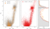 |
Fig. 15. Colour-magnitude diagrams (CMDs; left and middle) and absolute magnitude MK normalised histograms (right), where MK is estimated by means of the Gaia parallax at face value for the Kepler (grey) and C3 (orange) fields. Another CMD, including a shift in parallax, is shown for Kepler (red). We removed stars having a parallax with a relative error above 10% for Kepler, and 15% for C3. The black dashed lines indicate the expected range of values for the magnitude of the clump in the K band. |
6. Joint calibration of the seismic scaling relations and of the zero-point in the Gaia parallaxes
In Sect. 4.1, we used the scaling relations (Eqs. (4) and (5)) at face value in the context of a comparison with Gaia DR2. These relations are not precisely calibrated yet, and testing their validity has been a very active topic in the field of asteroseismology (e.g. Huber et al. 2012; Miglio 2012; Gaulme et al. 2016; Sahlholdt et al. 2018). In this vein, Gaia DR2 ensures the continuity of the research effort carried out to test the scaling relations’ accuracy. After the work conducted in Sects. 4 and 5, it is clear that the calibration of scaling relations by means of Gaia requires the parallax zero-point to be characterised at the same time. Hence, the current investigation reflects two main developments: constraining the calibration of the seismic scaling relations and quantifying the parallax offset in Gaia DR2.
We take the seismic calibration issue into account by introducing the scaling factors 𝒞⟨Δν⟩ and 𝒞νmax in the expressions of ⟨Δν⟩ and νmax (Eqs. (1) and (2)):
 (16)
(16)
 (17)
(17)
In terms of mass and radius (Eqs. (4) and (5)), this translates into
 (18)
(18)
 (19)
(19)
Finally, the seismic parallax (Eq. (6)) is modified as follows:
 (20)
(20)
In this context, the comparison between the Gaia (Eq. (3)) and asteroseismic (Eq. (20)) expressions for the parallax gives the following equality:
 (21)
(21)
where 𝒪Gaia represents the parallax zero-point in Gaia DR2 to be determined. Fitting Eq. (21) with a RANSAC algorithm allows us to determine the coefficient  , accounting for the calibration of scaling relations, and also provides an offset 𝒪Gaia, which we can interpret as a bias in the Gaia parallaxes. The main assumption that we make here is that the asteroseismic calibration, in the form of a multiplication factor, and the astrometric calibration, in the form of an addition factor, can be considered independently and do not affect each other. For this reason, it is crucial to make efficient use of both asteroseismic and astrometric data. On the one hand, because corrections to the scaling relations are expected to depend on νmax (see e.g. Fig. 3 of Rodrigues et al. 2017), we divided our Kepler RGB and RC samples in frequency ranges of νmax values: [8, 32], [16, 64], [32, 128], [64, 256], [128, 512] μHz. On the other hand, nearby stars have more reliable parallaxes (less affected, in relative terms, by the Gaia offset) and may, as such, be used to calibrate the scalings. In practice, we implemented a two-step methodology to, firstly, calibrate the seismic scaling relations and, secondly, use the calibration coefficients obtained from the first step to determine the Gaia zero-point. To do so, we started by selecting stars with large parallaxes in each bin of νmax. As illustrated by Fig. 16, the high-parallax threshold has to be chosen differently depending on the νmax bin considered, in order to keep enough stars. Here, the limit is chosen in such a way that at least 500 stars remain in the different νmax ranges. We then interpolate in νmax to estimate the scaling factors and individually correct each seismic parallax. The latter is then compared again to the Gaia parallax, this time on the full range of parallaxes, to measure the parallax offset.
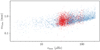 |
Fig. 16. ϖGaia as a function of νmax for RGB (blue) and RC (red) stars in the Kepler sample. |
During the calibration process, we apply linear fits expressed in the following form: ϖGaia = γϖscaling + δ, where  is the calibration parameter and δ = 𝒪Gaia is the offset parameter. The parameter uncertainties are estimated by repeating RANSACN = 1000 times, where we add a normally distributed noise knowing the observed uncertainties on ϖGaia and ϖscaling. The coefficients, obtained in step one, and offsets, obtained in step two, are shown as a function of νmax for RGB and RC stars in Fig. 17. The offsets 𝒪Gaia point in the right direction – Gaia parallaxes are smaller – and are in the same order of magnitude for the two evolutionary stages, validating the calibration of the scaling relations. These offsets do not depend on νmax, and their mean values are −24 ± 9 μas for RGB stars and −31 ± 7 μas for RC stars. In regard to the scaling factors, we can make a qualitative comparison with the 𝒞⟨Δν⟩ estimated from models if we assume 𝒞νmax to be equal to unity (uncertainties related to modelling the driving and damping of oscillations prevented theoretical tests of the νmax scaling relation; see e.g. Belkacem et al. 2011). According to Rodrigues et al. (2017; see their Fig. 3), 𝒞⟨Δν⟩ takes values slightly lower and higher than one for RGB and RC stars, respectively, in the ranges of mass and metallicity concerning our sample. Additionally, from RGB models, 𝒞⟨Δν⟩ is expected to decrease before increasing again as we go towards increasing νmax values, with a minimum at νmax ∼ 15 μHz depending on mass and metallicity. A similar trend is expected for RC stars but the other way around: 𝒞⟨Δν⟩ increases before decreasing, and has a maximum at νmax ∼ 30 μHz, which again depends on M and [Fe/H]. Also, larger variations of 𝒞⟨Δν⟩ are expected for RGB stars, which seems in conflict with our findings. Nevertheless, it should be recalled that we derived scaling factors that are averaged in bins of νmax, and it appears that the current results are still in general agreement with expectations from models. At this point, the third data release of Gaia, coming along with smaller uncertainties, will provide the means to pursue this work, and to derive precise and accurate corrections to the scaling relations.
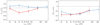 |
Fig. 17. Coefficients (left) and offsets (right) determined via our two-step calibration methodology for RGB (blue) and RC (red) stars, as a function of νmax. |
7. Conclusions
We combined Gaia and Kepler data to investigate the Gaia DR2 parallax zero-point, showing how the measured offsets depend on the asteroseismic method employed. We also provided a direct illustration of the positional dependence of the zero-point thanks to the K2 fields, and, finally, introduced a way to address the seismic and astrometric calibrations at the same time.
First of all, in the course of the comparison with the astrometric parallaxes delivered by the second data release of Gaia, the application of three distinct asteroseismic methods reveals that there is no absolute standard within asteroseismology. The determination of a zero-point in the Gaia parallaxes depends on the seismic approach used, and cannot be dissociated from it. As a matter of fact, the conclusions we draw are not the same whether we use the seismic scaling relations at face value or a grid-based method such as PARAM. The former would suggest a near-zero offset for RGB stars, significantly different from that of RC stars; in contrast, the latter implies a similar deviation with respect to Gaia DR2 parallaxes for RGB and RC stars. That said, the offsets measured with PARAM ranging from ∼ − 45 to −55 μas (and also considering the substantial uncertainties induced by spatially-correlated errors) can be related to previous investigations, especially the one conducted by Zinn et al. (2019), who calibrate seismic radii against eclipsing binary data in clusters and used model-predicted corrections on the ⟨Δν⟩ scaling relation. They obtain very similar offsets of about −50 μas for RGB and RC stars observed by Kepler. Our external validation via the measurements from eclipsing binaries in the open clusters NGC 6791 and NGC 6819 also confirms the existence of a parallax offset in that range. The proximity of the PARAM results with these independent tests reaffirms previous findings about the necessity to go beyond the ⟨Δν⟩ scaling for the estimation of stellar properties. Furthermore, the use of different sets of ⟨Δν⟩ values has a non-negligible impact on the inferred offsets of the order of ∼10 μas. In particular, attention should be paid to the consistency in the definition of ⟨Δν⟩ between the observations and the models. Other systematic effects can arise, for example, from shifts in the effective temperature and metallicity scales, and changes in the physical inputs of the models, with variations up to ±7 μas according to our tests, but very likely larger than that due to uncertainties related to stellar models.
We also bring to light the positional dependence of the Gaia DR2 parallax zero-point, as demonstrated by Lindegren et al. (2018), by analysing two of the K2 Campaign fields, C3 and C6, in addition to the Kepler field. These fields, corresponding to the south and north Galactic caps, display parallax offsets which are substantially different from that of Kepler. A small fraction of these differences may be due, for example, to the parallax distribution, the quality of the seismic data, and the use of different seismic constraints. But, as of now, it remains difficult to reach a firm conclusion, and the future possibility of extending this analysis to other K2 Campaign fields may help shed light on this matter. Also, despite the measured values being slightly different, the offset suggested by quasars reproduces the trend towards the increasing discrepancy with Gaia for C3, C6, and Kepler (in ascending order). The difference in the calculated zero-point is to be expected because quasars have their own peculiarities (e.g. faint magnitude, blue colour) that are not representative of red-giant stars. Furthermore, such a colour dependence also emerges from the study of δ Scuti stars in the Kepler field by Murphy et al. (2019), who found that applying an offset (as high as 30 μas) resulted in unrealistically low luminosities. Looking forward, having a uniform set of spectroscopic constraints would be very valuable.
Lastly, we initiate a two-step model-independent method to simultaneously calibrate the asteroseismic scaling relations and measure the Gaia DR2 parallax zero-point based on the assumption that these two corrections are fully decoupled. This leads us to promising findings whereby the computed calibration coefficients are qualitatively comparable to those that are derived from models, and the estimated offsets are in the same order of magnitude for RGB and RC stars suggesting that Gaia parallaxes are too small, as is expected. However, given the non-negligible uncertainties and the close correlation between the calibration and offset parameters, it is still too soon to draw strong conclusions. In this regard, the third data release of Gaia, with improved parallax uncertainties and reduced systematics, will offer exciting prospects to continue along the path of calibrating the scaling relations.
https://www.cosmos.esa.int/web/gaia/dr2-known-issues (slide 35).
Acknowledgments
This work has made use of data from the European Space Agency (ESA) mission Gaia (https://www.cosmos.esa.int/gaia), processed by the Gaia Data Processing and Analysis Consortium (DPAC, https://www.cosmos.esa.int/web/gaia/dpac/consortium). Funding for the DPAC has been provided by national institutions, in particular the institutions participating in the Gaia Multilateral Agreement. SK, AM, BM, GRD, BMR, DB, and LG are grateful to the International Space Science Institute (ISSI) for support provided to the asteroSTEP ISSI International Team. AM, WJC, GRD, BMR, YPE, and TSHN acknowledge the support of the UK Science and Technology Facilities Council (STFC). AM acknowledges support from the ERC Consolidator Grant funding scheme (project ASTEROCHRONOMETRY, G.A. n. 772293). LC is the recipient of the ARC Future Fellowship FT160100402. TSR acknowledges financial support from Premiale 2015 MITiC (PI B. Garilli). This work was supported by FCT/MCTES through national funds and by FEDER – Fundo Europeu de Desenvolvimento Regional through COMPETE2020 – Programa Operacional Competitividade e Internacionalização by grants: UID/FIS/04434/2019; PTDC/FIS-AST/30389/2017 & POCI-01-0145-FEDER-030389. DB is supported in the form of a work contract funded by national funds through Fundação para a Ciência e Tecnologia (FCT). We also wish to thank the referee whose comments helped clarify the paper and further interpret the results.
References
- Abolfathi, B., Aguado, D. S., Aguilar, G., et al. 2018, ApJS, 235, 42 [NASA ADS] [CrossRef] [Google Scholar]
- Arenou, F., Luri, X., Babusiaux, C., et al. 2018, A&A, 616, A17 [Google Scholar]
- Basu, S., Chaplin, W. J., & Elsworth, Y. 2010, ApJ, 710, 1596 [NASA ADS] [CrossRef] [Google Scholar]
- Belkacem, K. 2012, in SF2A-2012: Proceedings of the Annual meeting of the French Society of Astronomy and Astrophysics, eds. S. Boissier, P. de Laverny, & N. Nardetto, et al., 173 [Google Scholar]
- Belkacem, K., Goupil, M. J., Dupret, M. A., et al. 2011, A&A, 530, A142 [NASA ADS] [CrossRef] [EDP Sciences] [Google Scholar]
- Belkacem, K., Samadi, R., Mosser, B., Goupil, M. J., & Ludwig, H. G. 2013, ASP Conf. Ser., 479, 61 [Google Scholar]
- Brogaard, K., Bruntt, H., Grundahl, F., et al. 2011, A&A, 525, A2 [NASA ADS] [CrossRef] [EDP Sciences] [Google Scholar]
- Brogaard, K., VandenBerg, D. A., Bruntt, H., et al. 2012, A&A, 543, A106 [NASA ADS] [CrossRef] [EDP Sciences] [Google Scholar]
- Brogaard, K., Jessen-Hansen, J., Handberg, R., et al. 2016, Astron. Nachr., 337, 793 [NASA ADS] [CrossRef] [Google Scholar]
- Brogaard, K., Hansen, C. J., Miglio, A., et al. 2018, MNRAS, 476, 3729 [NASA ADS] [CrossRef] [Google Scholar]
- Brown, T. M., Gilliland, R. L., Noyes, R. W., & Ramsey, L. W. 1991, ApJ, 368, 599 [NASA ADS] [CrossRef] [Google Scholar]
- Cantat-Gaudin, T., Jordi, C., Vallenari, A., et al. 2018, A&A, 618, A93 [NASA ADS] [CrossRef] [EDP Sciences] [Google Scholar]
- Casagrande, L., & VandenBerg, D. A. 2014, MNRAS, 444, 392 [NASA ADS] [CrossRef] [MathSciNet] [Google Scholar]
- Casagrande, L., & VandenBerg, D. A. 2018a, MNRAS, 479, L102 [NASA ADS] [CrossRef] [Google Scholar]
- Casagrande, L., & VandenBerg, D. A. 2018b, MNRAS, 475, 5023 [NASA ADS] [CrossRef] [Google Scholar]
- Casagrande, L., Wolf, C., Mackey, A. D., et al. 2019, MNRAS, 482, 2770 [NASA ADS] [Google Scholar]
- Chen, Y. Q., Casagrande, L., Zhao, G., et al. 2017, ApJ, 840, 77 [NASA ADS] [CrossRef] [Google Scholar]
- Christensen-Dalsgaard, J. 2002, Rev. Mod. Phys., 74, 1073 [NASA ADS] [CrossRef] [Google Scholar]
- Davies, G. R., Silva Aguirre, V., Bedding, T. R., et al. 2016, MNRAS, 456, 2183 [NASA ADS] [CrossRef] [Google Scholar]
- Davies, G. R., Lund, M. N., Miglio, A., et al. 2017, A&A, 598, L4 [NASA ADS] [CrossRef] [EDP Sciences] [Google Scholar]
- De Ridder, J., Molenberghs, G., Eyer, L., & Aerts, C. 2016, A&A, 595, L3 [NASA ADS] [CrossRef] [EDP Sciences] [Google Scholar]
- Elsworth, Y., Hekker, S., Basu, S., & Davies, G. R. 2017, MNRAS, 466, 3344 [NASA ADS] [CrossRef] [Google Scholar]
- Farmer, R., Kolb, U., & Norton, A. J. 2013, MNRAS, 433, 1133 [NASA ADS] [CrossRef] [Google Scholar]
- Fischler, M. A., & Bolles, R. C. 1981, Commun. ACM, 24, 381 [Google Scholar]
- Gai, N., Basu, S., Chaplin, W. J., & Elsworth, Y. 2011, ApJ, 730, 63 [NASA ADS] [CrossRef] [Google Scholar]
- Gaia Collaboration (Brown, A. G. A., et al.) 2016a, A&A, 595, A2 [NASA ADS] [CrossRef] [EDP Sciences] [Google Scholar]
- Gaia Collaboration (Prusti, T., et al.) 2016b, A&A, 595, A1 [NASA ADS] [CrossRef] [EDP Sciences] [Google Scholar]
- Gaia Collaboration (Brown, A. G. A., et al.) 2018, A&A, 616, A1 [NASA ADS] [CrossRef] [EDP Sciences] [Google Scholar]
- Gaulme, P., McKeever, J., Jackiewicz, J., et al. 2016, ApJ, 832, 121 [NASA ADS] [CrossRef] [Google Scholar]
- Girardi, L. 2016, ARA&A, 54, 95 [NASA ADS] [CrossRef] [EDP Sciences] [Google Scholar]
- Girardi, L., Bertelli, G., Bressan, A., et al. 2002, A&A, 391, 195 [NASA ADS] [CrossRef] [EDP Sciences] [Google Scholar]
- Green, G. M., Schlafly, E. F., Finkbeiner, D. P., et al. 2015, ApJ, 810, 25 [NASA ADS] [CrossRef] [Google Scholar]
- Guggenberger, E., Hekker, S., Basu, S., & Bellinger, E. 2016, MNRAS, 460, 4277 [NASA ADS] [CrossRef] [Google Scholar]
- Hall, O. J., Davies, G. R., Elsworth, Y. P., et al. 2019, MNRAS, 486, 3569 [NASA ADS] [CrossRef] [Google Scholar]
- Handberg, R., Brogaard, K., Miglio, A., et al. 2017, MNRAS, 472, 979 [NASA ADS] [CrossRef] [Google Scholar]
- Hawkins, K., Leistedt, B., Bovy, J., & Hogg, D. W. 2017, MNRAS, 471, 722 [NASA ADS] [CrossRef] [Google Scholar]
- Hekker, S., Elsworth, Y., Mosser, B., et al. 2012, A&A, 544, A90 [NASA ADS] [CrossRef] [EDP Sciences] [Google Scholar]
- Howell, S. B., Sobeck, C., Haas, M., et al. 2014, PASP, 126, 398 [NASA ADS] [CrossRef] [Google Scholar]
- Huber, D., Ireland, M. J., Bedding, T. R., et al. 2012, ApJ, 760, 32 [NASA ADS] [CrossRef] [Google Scholar]
- Huber, D., Zinn, J., Bojsen-Hansen, M., et al. 2017, ApJ, 844, 102 [NASA ADS] [CrossRef] [Google Scholar]
- Kjeldsen, H., & Bedding, T. R. 1995, A&A, 293, 87 [NASA ADS] [Google Scholar]
- Lagarde, N., Miglio, A., Eggenberger, P., et al. 2015, A&A, 580, A141 [NASA ADS] [CrossRef] [EDP Sciences] [Google Scholar]
- Lindegren, L., Lammers, U., Bastian, U., et al. 2016, A&A, 595, A4 [NASA ADS] [CrossRef] [EDP Sciences] [Google Scholar]
- Lindegren, L., Hernández, J., Bombrun, A., et al. 2018, A&A, 616, A2 [NASA ADS] [CrossRef] [EDP Sciences] [Google Scholar]
- Luri, X., Brown, A. G. A., Sarro, L. M., et al. 2018, A&A, 616, A9 [NASA ADS] [CrossRef] [EDP Sciences] [Google Scholar]
- Majewski, S. R., Zasowski, G., & Nidever, D. L. 2011, ApJ, 739, 25 [NASA ADS] [CrossRef] [MathSciNet] [Google Scholar]
- Miglio, A. 2012, Astrophys. Space Sci. Proc., 26, 11 [NASA ADS] [CrossRef] [Google Scholar]
- Miglio, A., Montalbán, J., Carrier, F., et al. 2010, A&A, 520, L6 [NASA ADS] [CrossRef] [EDP Sciences] [Google Scholar]
- Miglio, A., Brogaard, K., Stello, D., et al. 2012, MNRAS, 419, 2077 [NASA ADS] [CrossRef] [Google Scholar]
- Miglio, A., Chaplin, W. J., Brogaard, K., et al. 2016, MNRAS, 461, 760 [NASA ADS] [CrossRef] [Google Scholar]
- Mosser, B., Belkacem, K., Goupil, M. J., et al. 2011, A&A, 525, L9 [NASA ADS] [CrossRef] [EDP Sciences] [Google Scholar]
- Murphy, S. J., Hey, D., Van Reeth, T., & Bedding, T. R. 2019, MNRAS, 485, 2380 [NASA ADS] [CrossRef] [Google Scholar]
- Pinsonneault, M. H., Elsworth, Y. P., Tayar, J., et al. 2018, ApJS, 239, 32 [NASA ADS] [CrossRef] [Google Scholar]
- Rendle, B. M., Miglio, A., Chiappini, C., et al. 2019, MNRAS, submitted [arXiv:1906.07489] [Google Scholar]
- Riello, M., De Angeli, F., Evans, D. W., et al. 2018, A&A, 616, A3 [NASA ADS] [CrossRef] [EDP Sciences] [Google Scholar]
- Riess, A. G., Casertano, S., Yuan, W., et al. 2018, ApJ, 861, 126 [Google Scholar]
- Rodrigues, T. S., Girardi, L., Miglio, A., et al. 2014, MNRAS, 445, 2758 [NASA ADS] [CrossRef] [Google Scholar]
- Rodrigues, T. S., Bossini, D., Miglio, A., et al. 2017, MNRAS, 467, 1433 [NASA ADS] [Google Scholar]
- Sahlholdt, C. L., Silva Aguirre, V., Casagrande, L., Mosumgaard, J. R., & Bojsen-Hansen, M. 2018, MNRAS, 476, 1931 [NASA ADS] [CrossRef] [Google Scholar]
- Sharma, S., Stello, D., Bland-Hawthorn, J., Huber, D., & Bedding, T. R. 2016, ApJ, 822, 15 [NASA ADS] [CrossRef] [Google Scholar]
- Silva Aguirre, V., Casagrande, L., Basu, S., et al. 2012, ApJ, 757, 99 [NASA ADS] [CrossRef] [Google Scholar]
- Skrutskie, M. F., Cutri, R. M., Stiening, R., et al. 2006, AJ, 131, 1163 [NASA ADS] [CrossRef] [Google Scholar]
- Stassun, K. G., & Torres, G. 2018, ApJ, 862, 61 [NASA ADS] [CrossRef] [Google Scholar]
- Stello, D., Chaplin, W. J., Bruntt, H., et al. 2009, ApJ, 700, 1589 [NASA ADS] [CrossRef] [Google Scholar]
- Stello, D., Huber, D., Sharma, S., et al. 2015, ApJ, 809, L3 [NASA ADS] [CrossRef] [Google Scholar]
- Stello, D., Vanderburg, A., Casagrande, L., et al. 2016, ApJ, 832, 133 [NASA ADS] [CrossRef] [Google Scholar]
- Stello, D., Zinn, J., Elsworth, Y., et al. 2017, ApJ, 835, 83 [NASA ADS] [CrossRef] [Google Scholar]
- Tassoul, M. 1980, ApJS, 43, 469 [NASA ADS] [CrossRef] [Google Scholar]
- Ulrich, R. K. 1986, ApJ, 306, L37 [NASA ADS] [CrossRef] [Google Scholar]
- Vandakurov, Y. V. 1967, AZh, 44, 786 [NASA ADS] [Google Scholar]
- Vrard, M., Mosser, B., Barban, C., et al. 2015, A&A, 579, A84 [NASA ADS] [CrossRef] [EDP Sciences] [Google Scholar]
- White, T. R., Bedding, T. R., Stello, D., et al. 2011, ApJ, 743, 161 [NASA ADS] [CrossRef] [Google Scholar]
- Yu, J., Huber, D., Bedding, T. R., et al. 2018, ApJS, 236, 42 [NASA ADS] [CrossRef] [Google Scholar]
- Zinn, J. C., Pinsonneault, M. H., Huber, D., & Stello, D. 2019, ApJ, 878, 136 [NASA ADS] [CrossRef] [Google Scholar]
All Tables
Values of (mean value of the stellar parameter X) for RGB (top) and RC stars (bottom).
All Figures
|
Fig. 1. Relative difference in ⟨Δν⟩, δ(Δν)/Δν = (Δνother − ΔνD16)/ΔνD16, between individual frequencies following Davies et al. (2016, D16) and another method, as a function of νmax as estimated by Mosser et al. (2011). The comparison is done with Mosser et al. (2011, M11; top) and Yu et al. (2018, Y18; bottom). RGB and RC stars are in blue and red, respectively. Here, Δν is used, instead of ⟨Δν⟩, to simplify the notation. |
| In the text | |
|
Fig. 2. Parallax difference ϖGaia − ϖseismo for RGB stars, with the asteroseismic parallax derived from raw scaling relations, as a function of ϖGaia, G, νmax, GBP − GRP, MPARAM, and [Fe/H]. The distribution of the N realisations of the RANSAC algorithm is indicated by the grey-shaded region and the yellow line displays the average linear fit, for which the relation is given at the top of each subplot. The values of |
| In the text | |
|
Fig. 3. Same as Fig. 2 but for RC stars. The values of |
| In the text | |
|
Fig. 4. ϖGaia as a function of ϖscaling (left) and ϖPARAM (right), for RGB (top) and RC (bottom) stars. The yellow line indicates the linear fit, averaged over N realisations, for which the relation is given at the top of each subplot. The black dashed line indicates the 1:1 relation. |
| In the text | |
|
Fig. 5. Re-normalised Unit Weight Error (RUWE) distribution for Kepler RGB and RC stars. The vertical dashed line indicates the threshold adopted: RUWE ≤ 1.2. |
| In the text | |
|
Fig. 6. Absolute difference in AK between PARAM and another method, as a function of PARAM’s extinctions. The comparison is made with the Green et al. (2015) map (left) and the RJCE method (right). |
| In the text | |
|
Fig. 7. Same as Fig. 2 but with the asteroseismic parallax derived from scaling relations with a 2.7% correction factor applied to the ⟨Δν⟩ scaling. The summary statistics are: |
| In the text | |
|
Fig. 8. Same as Fig. 2 but with the asteroseismic parallax derived from PARAM (Rodrigues et al. 2017). The summary statistics are: |
| In the text | |
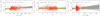 |
Fig. 9. Same as Fig. 8 but for RC stars. The summary statistics are: |
| In the text | |
|
Fig. 10. Slope of the various ϖseismo–ϖGaia relations as a function of the weighted average parallax difference for RGB (blue) and RC (red) stars. The results using raw scaling relations (crosses; Sect. 4.1), a corrected ⟨Δν⟩ scaling relation (circles; Sect. 4.2), and PARAM (diamonds; Sect. 4.3) are shown. For RC stars, the line is extended to lower offset values for a better visualisation of how the slope compares with RGB stars when using scaling relations at face value. |
| In the text | |
|
Fig. 11. ϖGaia as a function of ϖscaling (left) and ϖPARAM (right) for red giants in the K2 Campaign fields C3 (top) and C6 (bottom). The yellow line displays the linear fit, averaged over N realisations, for which the relation is given at the top of each subplot. The black dashed line indicates the 1:1 relation. The summary statistics are: |
| In the text | |
|
Fig. 12. Distribution of parallax uncertainties in Gaia DR2 (top) and in PARAM (bottom) for the Kepler (red), C3 (orange), and C6 (purple) fields. |
| In the text | |
|
Fig. 13. Sky map in ecliptic coordinates of median parallaxes for the full quasar sample, showing large-scale variations of the parallax zero-point. The Kepler (red), C3 (orange), and C6 (purple) fields are displayed. Median values are calculated in cells of 3.7 × 3.7 deg2. |
| In the text | |
|
Fig. 14. Weighted average parallax of quasars selected within a given radius around the central coordinates of the Kepler (red), C3 (orange), and C6 (purple) fields. The black dashed line indicates the average radius of the fields. |
| In the text | |
|
Fig. 15. Colour-magnitude diagrams (CMDs; left and middle) and absolute magnitude MK normalised histograms (right), where MK is estimated by means of the Gaia parallax at face value for the Kepler (grey) and C3 (orange) fields. Another CMD, including a shift in parallax, is shown for Kepler (red). We removed stars having a parallax with a relative error above 10% for Kepler, and 15% for C3. The black dashed lines indicate the expected range of values for the magnitude of the clump in the K band. |
| In the text | |
|
Fig. 16. ϖGaia as a function of νmax for RGB (blue) and RC (red) stars in the Kepler sample. |
| In the text | |
|
Fig. 17. Coefficients (left) and offsets (right) determined via our two-step calibration methodology for RGB (blue) and RC (red) stars, as a function of νmax. |
| In the text | |
Current usage metrics show cumulative count of Article Views (full-text article views including HTML views, PDF and ePub downloads, according to the available data) and Abstracts Views on Vision4Press platform.
Data correspond to usage on the plateform after 2015. The current usage metrics is available 48-96 hours after online publication and is updated daily on week days.
Initial download of the metrics may take a while.