| Issue |
A&A
Volume 628, August 2019
|
|
|---|---|---|
| Article Number | A116 | |
| Number of page(s) | 8 | |
| Section | Planets and planetary systems | |
| DOI | https://doi.org/10.1051/0004-6361/201731966 | |
| Published online | 14 August 2019 | |
Indications for transit-timing variations in the exo-Neptune HAT-P-26b★
1
Stellar Astrophysics Centre, Department of Physics and Astronomy, Aarhus University,
Ny Munkegade 120,
8000 Aarhus C, Denmark
e-mail: This email address is being protected from spambots. You need JavaScript enabled to view it.
2
Astronomical Observatory, Institute of Theoretical Physics and Astronomy, Vilnius University,
Sauletekio av. 3,
10257
Vilnius, Lithuania
3
Institute of Theoretical Astrophysics, University of Oslo,
Postboks 1029 Blindern,
0315 Oslo,
Norway
4
Facultad de Ciencias Astronómicas y Geofísicas, Universidad Nacional de La Plata,
Paseo del Bosque,
B1900FWA, La Plata, Argentina
5
Instituto de Astrofísica de La Plata (CCT-La Plata, CONICET-UNLP),
Paseo del Bosque, B1900FWA
La Plata, Argentina
6
Complejo Astronómico El Leoncito (CONICET-UNLP-UNC-UNSJ),
Av. España 1512 Sur, San Juan, Argentina
7
Institut für Astrophysik, Georg-August-Universität Göttingen,
Friedrich-Hund-Platz 1,
37077
Göttingen, Germany
8
Monash Centre for Astrophysics, School of Physics and Astronomy, Monash University,
Victoria 3800, Australia
9
Leibniz-Institut für Astrophysik Potsdam,
An der Sternwarte 16,
14482
Potsdam, Germany
Received:
18
September
2017
Accepted:
15
April
2019
Abstract
Upon its discovery, the low-density transiting Neptune HAT-P-26b showed a 2.1σ detection drift in its spectroscopic data, while photometric data showed a weak curvature in the timing residuals, the confirmation of which required further follow-up observations. To investigate this suspected variability, we observed 11 primary transits of HAT-P-26b between March, 2015, and July, 2018. For this, we used the 2.15 m Jorge Sahade Telescope placed in San Juan, Argentina, and the 1.2 m STELLA and the 2.5 m Nordic Optical Telescope, both located in the Canary Islands, Spain. To add to valuable information on the transmission spectrum of HAT-P-26b, we focused our observations in the R-band only. To contrast the observed timing variability with possible stellar activity, we carried out a photometric follow-up of the host star over three years. We carried out a global fit to the data and determined the individual mid-transit times focusing specifically on the light curves that showed complete transit coverage. Using bibliographic data corresponding to both ground and space-based facilities, plus our new characterized mid-transit times derived from parts-per-thousand precise photometry, we observed indications of transit timing variations in the system, with an amplitude of ~4 min and a periodicity of ~270 epochs. The photometric and spectroscopic follow-up observations of this system will be continued in order to rule out any aliasing effects caused by poor sampling and the long-term periodicity.
Key words: instrumentation: photometers / techniques: photometric / time / planets and satellites: fundamental parameters / stars: activity
The transit photometry (time, flux, error) and the long term monitoring in three bands are only available at the CDS via anonymous ftp to cdsarc.u-strasbg.fr (130.79.128.5) or via http://cdsarc.u-strasbg.fr/viz-bin/qcat?J/A+A/628/A116
© ESO 2019
1 Introduction
From the first exoplanets ever detected around stars other than our Sun, the most successful exoplanet detection methods have been the radial velocity (RV; e.g., Butler et al. 2006) and the transit (Charbonneau et al. 2000, and onward) techniques. The main engine of this work, the transit-timing variation (TTV) method, gained special relevance with the advent of the Kepler space telescope (Borucki et al. 2010; Koch et al. 2010). For this technique, once an exoplanet is detected via the transit method, the variations of the observed mid-transit times permit subsequent detection and/or characterization of further transiting (Carter et al. 2012) and nontransiting (Barros et al. 2014) exoplanets. The technique is sensitive to planets with masses as low that of Earth (Agol et al. 2005), which would be extremely challenging to detect or characterize by means of other techniques. The TTV method requires sufficiently long-baseline and precise photometry, and good phase coverage. All these requirements are satisfied by Kepler data (see e.g., Mazeh et al. 2013, for a TTV characterization of hundreds of Kepler objects of interest, KOIs). As a consequence, surveys focused on TTVs from the ground have been mainly carried out photometrically following-up hot Jupiters with deep transits orbiting bright stars (e.g., Maciejewski et al. 2011; Fukui et al. 2011; von Essen et al. 2013). Nonetheless, none of them have revealed unquestionable detection of TTVs. On the contrary, TTVs in the Kepler era have revealed that multiple systems are not rare at all, and that most of the planets in these multiple systems are within the Super Earth/mini Neptune regime (see Holman et al. 2010; Lissauer et al. 2011; Cochran et al. 2011). Therefore, from Kepler results we can re-focus our observing capabilities and boost our success rate from the ground by programming photometric follow-ups of more suitable transiting systems, including the Neptune planets, instead of only hot Jupiters.
Between 2015 and 2018 our group carried out a photometric follow-up of three Neptune-sized exoplanetary systems. The observations were mainly focused around primary transits. These systems presented either “hints” of multiplicity, or showed orbital and physical parameters similar to KOIs in multiple systems with large-amplitude TTVs. Here we present our efforts in the detection of TTVs in HAT-P-26b, which is one of such aforementioned systems. HAT-P-26b, a low-density Neptune-mass planet transiting a K-type star, and was discovered in 2011 by the HATNet consortia (Hartman et al. 2011). Once the spectral reconnaissance was carried out, additional high-resolution spectra were acquired to better characterize the RV variations and the stellar parameters. The spectroscopic analysis revealed a chromospherically quiet star, along with a Neptune-mass planet orbiting its host star every ~4.23 days. A combined analysis between photometric and spectroscopic data provided better constraints on the planetary mass and radius. Further analysis of spectroscopic data revealed a 2.1σ detection drift in its RVs. Nonetheless, the data were not sufficient to characterize the multiplicity of the system. Furthermore, Stevenson et al. (2016) observed a weak curvature in the timing residuals of HAT-P-26b, but yet again without proper confirmation due to insufficient data. Although the ΔF = 0.53% transit depth makes observation of the transit challenging using ground-based facilities, the observed RV drift and curvature in the timing residuals makes HAT-P-26b an interesting system for TTV studies. To confront the TTV detection with other possible sources of variability, we also carried out a photometric follow-up of the host star over three years.
Besides TTV analysis, several efforts were made to characterize the chemical constituents of the atmosphere of HAT-P-26b. While Stevenson et al. (2016) found tentative evidence for water and a lack of potassium in transmission, Wakeford et al. (2017) measured the atmospheric heavy element content of the planet and characterized its atmosphere as primordial. The observations presented here focused solely on the R-band. Thus, besides the TTV discovery and characterization, in this work we also provide an accurate wavelength-dependent planet-to-star radii ratio around the Johnson–Cousins R band, 635 ± 100 nm, in order to contribute to its exo-atmospheric characterization.
In this work, Sect. 2 details our observations and specifies the data-reduction techniques. Section 3 shows the steps involved in the transit analysis and the derived model parameters. Section 4 shows our results on TTVs, and we finish with a brief discussion and our conclusions in Sect. 5.
2 Observations and data reduction
2.1 Observing sites and specifications of the collected data for transit photometry
Between March, 2015, and July, 2018, we observed HAT-P-26 (R = 11.56, V = 11.76, Høg et al. 2000) during ten primary transits. Our observations were performed using the 2.15 m Jorge Sahade Telescope located at the Complejo Astronómico El Leoncito1 (CASLEO) in San Juan, Argentina, the 2.5 m Nordic Optical Telescope2 (NOT) located in La Palma, Spain, and the 1.2 m STELLA, located in Tenerife, Spain. The most relevant parameters of our observationsare summarized in Table 1. All the observations were carried out using a Johnson–Cousins R filter, to minimize the impact of our Earth’s atmosphere on the overall signal-to-noise ratio (S/N) of our measurements, circumventing telluric linesand the strong absorption of stellar light caused by Rayleigh scattering. Also, several transits allowed us to accurately characterize the size of HAT-P-26b within that wavelength range. To increase the photometric precision of our data, all telescopes were slightly defocused (Kjeldsen & Frandsen 1992; Southworth et al. 2009). In consequence, values of seeing taken from scienceframes are not representative of the quality of the sky at both sites. Table 1 shows then only intra night variability of the seeing. Exposure times were typically set between 10 and 60 s, and the photometricprecision ranged between 1.1 and 3.7 parts-per-thousand (ppt), in all cases below the transit depth (~5.3 ppt). Seven light curves show complete transit coverage. The rest show partial transit coverage mainly due to poor weather conditions.
During each observing night we obtained a set of 15 bias and between 10 and 15 twilight sky flats. Due to low exposure times and optimum cooling of charge-coupled devices, we did not take dark frames. In the case of CASLEO data we observed using a focal reducer. This produces an unvignetted field of view of 9 arcmin of diameter, allowing the simultaneous observation of HAT-P-26 along with two reference stars of similar brightness, namely TYC 320-426-1 (V = 11.08, Høg et al. 2000) and TYC 320-1376-1 (V = 12.5, Høg et al. 2000), also observed by STELLA. On the contrary, the size of the field of view of the NOT is about 7 arcmin2. Therefore, we only observed TYC 320-426-1 and fainter reference stars simultaneously to HAT-P-26.
2.2 Transit data reduction and preparation
For details on the data reduction, we refer the reader to the description of DIP2 OL (von Essen et al. 2018). In brief, all the science frames were bias and flat-field calibrated using the IRAF task ccdproc. Owing to the large availability of calibration frames, we corrected the science frames of a given observing night with the calibrations taken during that particular night only. To produce photometric light curves we used the IRAF task apphot. We measured fluxes inside apertures centered on the target and all available reference stars within the field of view of the telescopes. Their sizes were set as a fraction of the full width at half maximum (FWHM) computed and averaged per night. In particular, the apertures were set between 0.7 and 5 times the FWHM, divided into ten equally spaced steps. For each one of the apertures we chose three different sky rings, their widths being one, two, and three times the FWHM. The inner radii of the sky ring was fixed to five times the FWHM.
Next, we produced differential light curves for the target and each combination of reference stars by dividing the flux of the target by the average of a given combination of fluxes from the reference stars. For each one of the light curves we computed the standard deviation of the residuals, which were obtained by dividing the differential light curve by a high-degree, time-dependent polynomial that was fitted to the whole data, including in-transit points, minimizing the sum of the squares of the residuals. In particular, the degree of the polynomial was chosen to account for the shallow transit depth and most of the systematic noise. After visually inspecting all the light curves, it was chosen to be a septic degree and was fixed during all nights. The final combination of reference stars and aperture was chosen by minimizing the standard deviation of the residual light curves. This process was performed for each transit individually. With the time set in Julian dates and the differential fluxes defined, we finally changed the magnitude of the error bars provided by the apphot task so that their average magnitude was coincident with the standard deviation of the data. Besides time, flux, and errors, we also computed (x,y) centroid positions, integrated flat counts in the selected aperture around those (x,y) positions, the seeing, the airmass, and the background counts inside the selected sky ring, all of them as a function of time and for all the stars involved in the selected differential light curve.
Relevant parameters of our observations.
2.3 Datareduction of the long-term monitoring of HAT-P-26
Stellar activity, and particularly stellar spots rotating with the star, can mimic TTVs (see Sect. 4.2). As part of the VAriability MOnitoring of exoplanet host Stars (VAMOS) project, we carried out a photometric follow-up of the host star, HAT-P-26, over three years. To this end we observed with the wide-field imager WIFSIP mounted at the 1.2 m twin-telescope STELLA located in the Canary Islands, Spain (Strassmeier et al. 2004; Weber et al. 2012). Table 2 shows the main characteristics of the observations. The data were reduced using standard routines of ESO-MIDAS. On average, around five stars were used to construct the differential light curve. For details on the data reduction steps, we refer the reader to Mallonn et al. (2015) and Mallonn & Strassmeier (2016).
3 Model parameters and transit analysis
3.1 Choice of detrending model and correlated noise treatment
To clean thedata from systematic errors we constructed an initial detrending model, DM, with its terms represented by a linear combination of seeing, S, airmass, χ, centroid positions of all the stars involved in the creation of the differential light curves (x,y), and their respective integrated flat counts and background counts around these positions, henceforth, the detrending components:
![Mathematical equation: \begin{eqnarray*} && \hspace*{-5pt}\textrm{DM}(t)\;{=}\;a_0 + a_1\times S\!\;{+}\; a_2 \times \chi\nonumber\\[3pt] && \hspace*{-5pt} \qquad\quad\;\; +\;\sum_1^{N+1} c_i\times {\textrm{BG}}_i + d_i \times {\textrm{FC}}_i + e_i \times X_i + f_i \times Y_i\,. \end{eqnarray*}](/articles/aa/full_html/2019/08/aa31966-17/aa31966-17-eq1.png) (1)
(1)
Here, N is the total number of reference stars and N + 1 includes the components of the target star. Xi and Yi correspond to the (x,y) centroid positions, FCi to the integrated flat counts, and BGi to the background counts. The coefficients of the detrending model are a0, a1, a2, and di, ei and fi, with i = 1, N + 1. Besides this linear combination, we also considered time-dependent polynomials with degrees ranging from one to three. The detrending strategy is fully described in von Essen et al. (2018). In an iterative process we defined a joint model described as the transit model (see Sect. 3.2 for details) multiplied by the detrending model. During each iteration, where we evaluated the different time-dependent polynomials and the different combinations of detrending components, we computed reduced χ2, the Bayesian information criterion (BIC; see e.g., von Essen et al. 2017, for details on its use) and the weighted standard deviation between the transit photometry and the combined model. In all these statistical indicators, the number of fitting parameters is taken into consideration. Thus, we made sure that the data were not being over-fitted by an unnecessarily large detrending model. After averaging the three statistical indicators, we chose as final detrending model (and thus, the final number of detrending components or the final degree for the time-dependent polynomial) the one that minimized this averaged statistic. Usually, the airmass, the (x,y) centroid positions, and the integrated flat counts of all the stars involved in the construction of the differential light curves were part of the chosen detrending model. For the NOT data, which counts with an excellent tracking system, a second-order, time-dependent polynomial was usually sufficient to account for instrumental systematics. Once the detrending model was defined, we treated correlated noise as specified in von Essen et al. (2013). Briefly, following Carter & Winn (2009) we produced residual light curves, subtracting the primary transit model from the data (Mandel & Agol 2002). As orbital parameters we used bibliographic values, listed in this work in the first column of Table 3. We then divided each light curve into M bins of equal duration, each bin holding an averaged number of N data points.An averaged N accounts for unequally spaced data points. If the data are free of correlated noise, then the noise within the residual light curves should follow the expectation of independent random numbers  ,
,
![Mathematical equation: \begin{equation*} \hat{\sigma_N}\,{=}\,\sigma_1 N^{-1/2}[M/(M-1)]^{1/2}. \end{equation*}](/articles/aa/full_html/2019/08/aa31966-17/aa31966-17-eq3.png) (2)
(2)
Here, σ1 is the sample variance of the unbinned data and σN is the sample variance (or RMS) of the binned data:
 (3)
(3)
where the mean value of the residuals per bin is given by  , and
, and  is the mean value of the means. When correlated noise cannot be neglected, each σN differs by some factor βN from their expectation
  . We computed β averaging the values of βN obtained over time bins close to the duration of the transit ingress (or, equivalently, egress) of HAT-P-26b, which is estimated to be ~15 min. To estimate β, we used time bins of 0.8, 0.9, 1, 1.1, and 1.2 times the duration of ingress. Finally, we enlarged the magnitude of the error bars by β (Pont et al. 2006). On average, CASLEO data presented slightly more correlated noise (β ~ 2.1) compared to the NOT (β ~ 1.5). This is explained by guiding the stars (see column eight of the Table 1 for a measurement of the amplitude of variability of the centroid position of the stars). While the NOT has a stable guiding system, CASLEO lacks guiding and the telescope slightly tracks in the east-west direction, affecting the quality of the photometry.
Main characteristics of the observations performed with STELLA.
Bibliographic and derived transit parameters of HAT-P-26b.
3.2 Transit fitting
With the ten light curves fully constructed, we converted the time stamps from Julian dates to Barycentric Julian dates, BJDTDB, using the web tool provided by Eastman et al. (2010). The first step was to determine the expectation values of the model parameters of HAT-P-26b. To this end, we carried out a Markov-chain Monte Carlo (MCMC) global fit using the PyAstronomy3 packages (Patil et al. 2010; Jones et al. 2001). As transit model we used the one provided by Mandel & Agol (2002), along with a quadratic limb-darkening law. In particular, for the Mandel & Agol (2002) transit model the fitting parameters are the inclination in degrees, i, the semi-major axis in stellar radius, a∕RS, the orbital period in days, Per, the planet-to-star radii ratio, RP /RS, the mid-transit time in BJDTDB, T0, and the linear and quadratic limb-darkening coefficients, u1 and u2.
The quadratic limb-darkening coefficients were taken from Claret (2000) for the Johnson–Cousins R filter and stellar parameters closely matching those of HAT-P-26 (Teff = 5079 ± 88 K, [Fe/H] = −0.04 ± 0.08, and log (g) = 4.56 ± 0.06, Hartman et al. 2011). Thus, the values for the limb-darkening coefficients used in this work correspond to the stellar parameters Teff = 5000 K, [Fe/H] = 0 and log (g) = 4.5, and are listed in Table 3. In this work, quadratic limb-darkening coefficients are considered as fixed values. Nonetheless, to test if the adopted values for the limb-darkening coefficients have an impact on the measured mid-transit times, we considered the linear and quadratic limb-darkening values as fitting parameters as well. After carrying out a global fit including them in the fitting process, our posterior distributions for the parameters revealed values inconsistent with the spectral classification of the host star. Although our data present a photometric precision at the parts-per-thousand level, the transit light curves are not precise enough to realistically fit for the limb-darkening coefficients. Nonetheless, mid-transit times computed fitting for the limb-darkening coefficients do not show a significant offset with respect to those computed to fix them, but they do show slightly larger error bars.
To fit the data with our combined model, we began our analysis considering the transit parameters listed in Hartman et al. (2011), Stevenson et al. (2016), and Wakeford et al. (2017) as starting values. The adopted values are shown in the second column of Table 3. We chose uniform priors for the orbital period, and Gaussian priors for the semi-major axis, the inclination, and the planet-to-star radii ratio. To be conservative and to avoid misleading the convergence of the fitting algorithm, as standard deviation for the Gaussian priors we chose three times the magnitude of the errors determined by the latter mentioned authors. The mid-transit time determined by Stevenson et al. (2016) has already five decimals of precision, which translates into an accuracy of ~2 s. Since this precision is significantly below our data cadence, throughout this work the reference mid-transit time is consider as fixed.
Once the priors were set, we iterated the fitting process 1.5 ×10⁵ times. At each MCMC step not only are the transit parameters changed, but also the detrending coefficients are computed with the previously mentioned inversion techniques. Both transit parameters and detrending coefficients are saved at each MCMC step. When the total number of iterations was reached, we burned the initial 50 000 samples. From the mean values and standard deviations of the samples we computed the expectation values of the model parameters and their corresponding errors. The same process was followed to determine the best-fit detrending coefficients. Throughout this work we provide the errors of the transit parameters at 1σ level. As a consistency check we analyzed the posterior distributions to ensure convergence of the chains. To this end, we divided the chains in three equally large fractions, we computed the model parameters for each one of the sub-chains, and we checked that they were consistent within 1σ errors. Our best-fit values are listed in the third column of Table 3. To avoid visual contamination, not all the values for the transit parameters derived by other authors are displayed in Table 3. Nonetheless, the transit parameters presented in this work are in good agreement with all the bibliographic values. In particular, the value for the planet-to-star radii ratio follows the trend observed by Wakeford et al. (2017), and not the value reported by Hartman et al. (2011). Figure 1 shows one transit light curve and both model components in isolation.
After producing a global fit to the complete data set (see Sect. 3.2), to characterize possible TTVs in the system we proceeded to fit the transits individually. Figure 2 shows the 11 transits, 7 of them corresponding to the JS telescope(red circles), 1 to STELLA (blue circles) and the remaining 4 to the NOT (green squares). To provide TTVs that are as realistic as possible, for this analysis we fitted each individual transit. However, for a better assessment of the TTVs, complete and incomplete transits are clearly differentiated.
To compute the mid-transit times of the individual light curves, rather than considering our best-fit model parameters as fixed, we used our global best-fit values and errors for the mean and standard deviation, respectively, for the Gaussian priors. For each individual mid-transit time we chose uniform priors. Since the determination of the individual mid-transit times requires the analysis of individual light curves, the orbital period was considered as fixed to the value derived from the global fit. This will properly propagate the uncertainties of all the transit parameters into the determination of the mid-transit times and thus will provide more realistic uncertainties. Equivalently to the global fit, we iterated and burned the same number of chains per light curve, and we computed the individual mid-transit times in the same fashion as specified in Sect. 3.2. For each light curve we also computed the transit parameters and checked that they were consistent with the global ones, always at 1σ level. The first section of Table 4 shows the individual mid-transit times from the literature and their respective uncertainties, while the second section shows the mid-transit times and the uncertainties derived in this work.
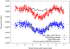 |
Fig. 1 Detrending process. The figure shows the evolution of the transit photometry during the fitting procedure. Raw data are plotted in red circles. The detrending model is plotted as a black continuous line. Artificially shifted, the detrended data are plotted as blue squares, along with primary transit models whose transit parameters are determined by the posterior distributions of the MCMC chains. |
4 Analysis and results
4.1 Transit timing variations
We computed the TTVs for the HAT-P-26b system by subtracting observed mid-transit times from mid-transit times obtained from a constant (best-fit) orbital period. The derived values can be found in Fig. 3and the lower part of Table 4. We note that in the figure the zeroth epoch does not lie over the abscissas axis. This is due to the improvement of its value between Hartman et al. (2011) and Wakeford et al. (2017).
In the absence of any timing variations we expect no significant deviations of the derived O–C values from zero. We used a  test to test the null hypothesis of O–C = 0. For 20 degrees of freedom the value raises up to
  = 177, with a p-value of P < 1 × 10⁻⁵. For this, the significance level is chosen to be 1%. This simple statistical analysis,
  , and its corresponding p-value indicate that the mid-transit times of HAT-P-26b are inconsistent with a constant period. Visual inspection of the O–C diagram for HAT-P-26b suggests that the TTVs are strongly dependent on the last three data points. To test these assumptions we excluded the three last epochs and re-computed our statistics:
  = 102, P < 1 × 10⁻⁵.
For completeness, assuming TTVs with a sinusoidal variability we fitted a simple sinusoidal function with the following expression to our timing residuals:
![Mathematical equation: \begin{equation*} \mathrm{TTVs}(E)\,{=}\,A_{\mathrm{TTVs}} \sin[2\pi(E/\textrm{Per}_{\mathrm{TTVs}} - \phi_{\mathrm{TTVs}})], \end{equation*}](/articles/aa/full_html/2019/08/aa31966-17/aa31966-17-eq12.png) (4)
(4)
where E corresponds to the epoch, ATTVs corresponds to the semi-amplitude of the timing residuals, PerTTVs to the periodicity, and ϕTTVs to the phase. From our analysis,we obtain ATTVs ~ 2.1 min, while the best-fit periodicity would correspond to around 270 epochs. This is equivalent to almost 1100 days. Comparing the semi-amplitude with the average error bars for the timings we find ATTVs ~ 3 × ɛ, ɛ being the averaged value of the timing errors. Our best-fit sinusoidal function is plotted in Fig. 3 as a black dashed line. Mainly due to possible aliasing effects, and due to the complications that single-transiting planets with TTVs convey, we believe any analysis on the TTVs reported in this work is subject to strong speculation. More spectroscopic and photometric data are required to characterize the body causing these TTVs.
4.2 Transit timing variations induced by stellar activity
Due to the high photometric quality provided by space-based observations such as CoRoT (Auvergne et al. 2009) and Kepler, stellar magnetic activity and its impact on transit light curves have been studied in great detail. Dark spots and bright feculae on the stellar photosphere move as the star rotates, producing a time-dependent variation of the stellar flux. The currently obtainable photometric precision is so high that the small imprints of occulted spots on transit data have been used to characterize stellar surface-brightness profiles and spot migration and evolution (see e.g., Carter et al. 2011; Sanchis-Ojeda et al. 2011; Sanchis-Ojeda & Winn 2011; Huber et al. 2010). When transit fitting is performed, an incorrect treatment of these “bumps” can have a significant impact on the computation of planetary and stellar parameters (see e.g., Czesla et al. 2009; Lanza 2011).
Occulted and unocculted spots can asymmetrically modify the shape of the transit light curves, and thus affect the true locations of the mid-transit times. Actually, the deformations that stellar activity produces on primary transits have been studied in detail and pinpointed in some cases as a misleading identification of TTVs (see e.g., Rabus et al. 2009). For example, Maciejewski et al. (2011) found TTVs in the WASP-10 system with an amplitude of a few minutes. These latter authors attributed the variability to the gravitational interaction between the transiting planet and a second body of a tenth of a Jupiter mass close to a 5:3 mean-motion resonance. Although Barros et al. (2013) did not find a linear ephemeris as a statistically good fit to the mid-transit times of WASP-10b, they showed that the observed variability could be produced by, for example, spot occultation features.
To quantify stellar activity in our system and support (or overrule) our TTV detection, we carried out a photometric follow-up of HAT-P-26 over three years (see e.g., Mallonn et al. 2015; Mallonn & Strassmeier 2016, Fig. 4 and our Table 2). The data, taken in the Johnson–Cousins B, V, and I filters, show a maximum scatter of 2.3 ppt. To search for any significant periodicity contained in the data we computed Lomb–Scargle periodograms (Lomb 1976; Scargle 1982; Zechmeister & Kürster 2009), finding featureless periodograms within each observing season and within the whole observing run. As a consequence, the photometric follow-up of the host star seems to show no evidence of spot modulation. Nonetheless, the characterization presented in this work is as good as the data are. In other words, if spot-induced modulation were to exist, it would be well contained within the ~2 ppm limit.
Hartman et al. (2011) characterized the chromospheric activity of the star derived from the flux in the cores of the Ca II H and K lines, the so-called S index, SHK = 0.182 ± 0.004. Comparing this value to the relation between the S index and the stellar brightness variation found by Karoff et al. (2016) (their Fig. 5), observational evidence should place the photometric variability of HAT-P-26 at around 1 ppt. Assuming that spot modulation around and below this limit actually exists, and that it might have an impact on the TTVs, Ioannidis et al. (2016) found that the maximum amplitude of TTVs generated by spot crossing events strongly depends on transit duration (among other things). In the case of HAT-P-26b (~143 min), TTVs caused by spots should have a maximum amplitude of ~1 min. This is significantly below the TTV amplitude detected in this work. Therefore, the data presented here seem to support a scenario where TTVs are caused by gravitational interactions instead of being modulated by the potential activity of the star.
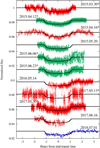 |
Fig. 2 11 transit light curves collected in this work. The transits observed with the Argentinian 2.15 m telescope, CASLEO, are plotted as red circles. The transits taken with the Scandinavian 2.5 m NOT are shown as green squares. The transit observed with STELLA is shown in blue circles. Calender dates are displayed, and asterisks indicate the transits that are complete. Vertical dashed lines indicate the four contact times to guide the reader. Transits have been folded using our best-fit orbital period. In consequence, TTVs can be appreciated by comparing ingress or egress to the vertical dashed lines. |
Fitted instant of minima with 1-σ errors and the O–C data points.
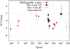 |
Fig. 3 Observed minus calculated (O–C) mid-transit times for HAT-P-26b in minutes. Red circular points show the values obtained from Hartman et al. (2011), Stevenson et al. (2016), and Wakeford et al. (2017). Black filled squares correspond to the values derived in this work considering complete transits, while empty squares are those derived from incomplete transits. The O–C diagram was computed using the best-fit orbital period derived in this work, specified in Table 3. The dashed black line corresponds to our best-fit sinusoidal variability. |
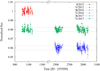 |
Fig. 4 Photometric follow-up of HAT-P-26 using the STELLA photometer. Red circles correspond to the I band, green squares to the V band, and blue triangles to the B band. The fluxes have been artificially shifted, and the time axis has been compressed for improved visualization. Dashed black lines show the averaged standard deviation. |
4.3 Transit timing variations caused by systematic effects
Besides stellar activity, TTVs can be caused by systematic effects not properly accounted for. This has a special relevance when low-amplitude TTVs are being reviewed. A manifestation of this effect is the derivation of underestimated error bars for the mid-transit times. While in this work we have taken special care over the computation of uncertainties, we can only trust that the values reported by other authors have received similar treatment. Nonetheless, as a consistency check we enlarged the error bars of all the observed mid-transit times by a factor and re-computed  for each one of the artificially enlarged O–C diagrams. A factor of 13 was required for
  to be consistent with 1, equivalently, with no TTVs. This marginally relatively large value seems to support our TTV detection.
5 Discussion and conclusions
Since its discovery, indications of variability in both spectroscopic and photometric data have flagged HAT-P-26b as an interesting target for additional photometric follow-up. For the last three years our group has been collecting primary transit data of parts-per-thousand photometric precision, necessary to detect the shallow transits that the planet produces while crossing its host star every ~4.23 days. In this study we reduced all the new data in a homogeneous way, updated and improved the transit parameters and ephemeris, and detected significant variability in the timing residuals. Furthermore, we followed the host star over several years to characterize its activity and, if observed, its impact on mid-transit times. However, light curves taken in three different bands over three years revealed no spot modulation within the precision limit of the data, devaluing the scenario of spot-induced TTVs. Due to the complexity of the analysis of single-transiting systems presenting TTVs, it is hard to make any robust conclusions on the characteristics of the perturbing body. Nonetheless, we understand these results to be relevant and to motivate future photometric and spectroscopic follow-up campaigns that will contribute to disclosing the origin of the observed variability.
Acknowledgements
Visiting Astronomer, Complejo Astronómico El Leoncito operated under agreement between the Consejo Nacional de Investigaciones Científicas y Técnicas de la República Argentina and the National Universities of La Plata, Córdoba and San Juan. C.v.E. acknowledges funding for the Stellar Astrophysics Centre, provided by The Danish National Research Foundation (Grant DNRF106), and support from the European Social Fund via the Lithuanian Science Council grant No. 09.3.3-LMT-K-712-01-0103. This study is based on observations made with the NOT, operated by the Nordic Optical Telescope Scientific Association at the Observatorio del Roque de los Muchachos, La Palma, Spain, of the Instituto de Astrofisica de Canarias. We acknowledge support from the Research Council of Norway’s grant 188910 to finance service observing at the NOT. S.W. acknowledges support for International Team 265 (“Magnetic Activity of M-type Dwarf Stars and the Influence on Habitable Extra-solar Planets”) funded by the International Space Science Institute (ISSI) in Bern, Switzerland, and support by the Research Council of Norway through its Centres of Excellence scheme, project number 262622. V.P. wishes to acknowledge the funding that was provided in part by a J. William Fulbright Grant and the sponsorship of Georg-August-Universitat in Gottingen, Germany. We thank the referee for comments which contributed to improving this work. This work made use of PyAstronomy4.
References
- Agol, E., Steffen, J., Sari, R., & Clarkson, W. 2005, MNRAS, 359, 567 [NASA ADS] [CrossRef] [Google Scholar]
- Auvergne, M., Bodin, P., Boisnard, L., et al. 2009, A&A, 506, 411 [NASA ADS] [CrossRef] [EDP Sciences] [Google Scholar]
- Barros, S. C. C., Boué, G., Gibson, N. P., et al. 2013, MNRAS, 430, 3032 [NASA ADS] [CrossRef] [Google Scholar]
- Barros, S. C. C., Díaz, R. F., Santerne, A., et al. 2014, A&A, 561, L1 [NASA ADS] [CrossRef] [EDP Sciences] [Google Scholar]
- Borucki, W. J., Koch, D., Basri, G., et al. 2010, Science, 327, 977 [NASA ADS] [CrossRef] [PubMed] [Google Scholar]
- Butler, R. P., Wright, J. T., Marcy, G. W., et al. 2006, ApJ, 646, 505 [NASA ADS] [CrossRef] [Google Scholar]
- Carter, J. A., & Winn, J. N. 2009, ApJ, 704, 51 [NASA ADS] [CrossRef] [Google Scholar]
- Carter, J. A., Winn, J. N., Holman, M. J., et al. 2011, ApJ, 730, 82 [NASA ADS] [CrossRef] [Google Scholar]
- Carter, J. A., Agol, E., Chaplin, W. J., et al. 2012, Science, 337, 556 [NASA ADS] [CrossRef] [PubMed] [Google Scholar]
- Charbonneau, D., Brown, T. M., Latham, D. W., & Mayor, M. 2000, ApJ, 529, L45 [NASA ADS] [CrossRef] [PubMed] [Google Scholar]
- Claret, A. 2000, A&A, 363, 1081 [NASA ADS] [Google Scholar]
- Cochran, W. D., Fabrycky, D. C., Torres, G., et al. 2011, ApJS, 197, 7 [NASA ADS] [CrossRef] [Google Scholar]
- Czesla, S., Huber, K. F., Wolter, U., Schröter, S., & Schmitt, J. H. M. M. 2009, A&A, 505, 1277 [NASA ADS] [CrossRef] [EDP Sciences] [Google Scholar]
- Eastman, J., Siverd, R., & Gaudi, B. S. 2010, PASP, 122, 935 [NASA ADS] [CrossRef] [Google Scholar]
- Fukui, A., Narita, N., Tristram, P. J., et al. 2011, PASJ, 63, 287 [NASA ADS] [Google Scholar]
- Hartman, J. D., Bakos, G. Á., Kipping, D. M., et al. 2011, ApJ, 728, 138 [NASA ADS] [CrossRef] [Google Scholar]
- Høg, E., Fabricius, C., Makarov, V. V., et al. 2000, A&A, 355, L27 [Google Scholar]
- Holman, M. J., Fabrycky, D. C., Ragozzine, D., et al. 2010, Science, 330, 51 [NASA ADS] [CrossRef] [PubMed] [Google Scholar]
- Huber, K. F., Czesla, S., Wolter, U., & Schmitt, J. H. M. M. 2010, A&A, 514, A39 [NASA ADS] [CrossRef] [EDP Sciences] [Google Scholar]
- Ioannidis, P., Huber, K. F., & Schmitt, J. H. M. M. 2016, A&A, 585, A72 [NASA ADS] [CrossRef] [EDP Sciences] [Google Scholar]
- Jones, E., Oliphant, T., Peterson, P., et al. 2001, SciPy: Open source scientific tools for Python, http://www.scipy.org [Google Scholar]
- Karoff, C., Knudsen, M. F., De Cat, P., et al. 2016, Nat. Commun., 7, 11058 [NASA ADS] [CrossRef] [Google Scholar]
- Kjeldsen, H., & Frandsen, S. 1992, PASP, 104, 413 [NASA ADS] [CrossRef] [Google Scholar]
- Koch, D. G., Borucki, W. J., Basri, G., et al. 2010, ApJ, 713, L79 [NASA ADS] [CrossRef] [Google Scholar]
- Lanza, A. F. 2011, in Physics of Sun and Star Spots, eds. D. Prasad Choudhary & K. G. Strassmeier, IAU Symp., 273, 89 [NASA ADS] [Google Scholar]
- Lissauer, J. J., Fabrycky, D. C., Ford, E. B., et al. 2011, Nature, 470, 53 [NASA ADS] [CrossRef] [PubMed] [Google Scholar]
- Lomb, N. R. 1976, Ap&SS, 39, 447 [NASA ADS] [CrossRef] [Google Scholar]
- Maciejewski, G., Dimitrov, D., Neuhäuser, R., et al. 2011, MNRAS, 411, 1204 [NASA ADS] [CrossRef] [Google Scholar]
- Mallonn, M., & Strassmeier, K. G. 2016, A&A, 590, A100 [NASA ADS] [CrossRef] [EDP Sciences] [Google Scholar]
- Mallonn, M., von Essen, C., Weingrill, J., et al. 2015, A&A, 580, A60 [NASA ADS] [CrossRef] [EDP Sciences] [Google Scholar]
- Mandel, K., & Agol, E. 2002, ApJ, 580, L171 [NASA ADS] [CrossRef] [Google Scholar]
- Mazeh, T., Nachmani, G., Holczer, T., et al. 2013, ApJS, 208, 16 [NASA ADS] [CrossRef] [Google Scholar]
- Patil, A., Huard, D., & Fonnesbeck, C. J. 2010, J. Stat. Softw., 35, 1 [CrossRef] [EDP Sciences] [Google Scholar]
- Pont, F., Zucker, S., & Queloz, D. 2006, MNRAS, 373, 231 [NASA ADS] [CrossRef] [Google Scholar]
- Rabus, M., Alonso, R., Belmonte, J. A., et al. 2009, A&A, 494, 391 [NASA ADS] [CrossRef] [EDP Sciences] [Google Scholar]
- Sanchis-Ojeda, R., & Winn, J. N. 2011, ApJ, 743, 61 [NASA ADS] [CrossRef] [Google Scholar]
- Sanchis-Ojeda, R., Winn, J. N., Holman, M. J., et al. 2011, ApJ, 733, 127 [NASA ADS] [CrossRef] [Google Scholar]
- Scargle, J. D. 1982, ApJ, 263, 835 [NASA ADS] [CrossRef] [Google Scholar]
- Southworth, J., Hinse, T. C., Jørgensen, U. G., et al. 2009, MNRAS, 396, 1023 [NASA ADS] [CrossRef] [Google Scholar]
- Stevenson, K. B., Bean, J. L., Seifahrt, A., et al. 2016, ApJ, 817, 141 [NASA ADS] [CrossRef] [Google Scholar]
- Strassmeier, K. G., Granzer, T., Weber, M., et al. 2004, Astron. Nachr., 325, 527 [NASA ADS] [CrossRef] [Google Scholar]
- von Essen, C., Schröter, S., Agol, E., & Schmitt, J. H. M. M. 2013, A&A, 555, A92 [NASA ADS] [CrossRef] [EDP Sciences] [Google Scholar]
- von Essen, C., Cellone, S., Mallonn, M., et al. 2017, A&A, 603, A20 [NASA ADS] [CrossRef] [EDP Sciences] [Google Scholar]
- von Essen, C., Ofir, A., Dreizler, S., et al. 2018, A&A, 615, A79 [NASA ADS] [CrossRef] [EDP Sciences] [Google Scholar]
- Wakeford, H. R., Sing, D. K., Kataria, T., et al. 2017, Science, 356, 628 [NASA ADS] [CrossRef] [Google Scholar]
- Weber, M., Granzer, T., & Strassmeier, K. G. 2012, in Software and Cyberinfrastructure for Astronomy II, Proc. SPIE, 8451, 84510K [CrossRef] [Google Scholar]
- Zechmeister, M., & Kürster, M. 2009, A&A, 496, 577 [NASA ADS] [CrossRef] [EDP Sciences] [Google Scholar]
Visiting Astronomer, Complejo Astronómico El Leoncito operated under agreement between the Consejo Nacional de Investigaciones Científicas y Técnicas de la República Argentina and the National Universities of La Plata, Córdoba and San Juan; www.casleo.gov.ar
All Tables
All Figures
|
Fig. 1 Detrending process. The figure shows the evolution of the transit photometry during the fitting procedure. Raw data are plotted in red circles. The detrending model is plotted as a black continuous line. Artificially shifted, the detrended data are plotted as blue squares, along with primary transit models whose transit parameters are determined by the posterior distributions of the MCMC chains. |
| In the text | |
|
Fig. 2 11 transit light curves collected in this work. The transits observed with the Argentinian 2.15 m telescope, CASLEO, are plotted as red circles. The transits taken with the Scandinavian 2.5 m NOT are shown as green squares. The transit observed with STELLA is shown in blue circles. Calender dates are displayed, and asterisks indicate the transits that are complete. Vertical dashed lines indicate the four contact times to guide the reader. Transits have been folded using our best-fit orbital period. In consequence, TTVs can be appreciated by comparing ingress or egress to the vertical dashed lines. |
| In the text | |
|
Fig. 3 Observed minus calculated (O–C) mid-transit times for HAT-P-26b in minutes. Red circular points show the values obtained from Hartman et al. (2011), Stevenson et al. (2016), and Wakeford et al. (2017). Black filled squares correspond to the values derived in this work considering complete transits, while empty squares are those derived from incomplete transits. The O–C diagram was computed using the best-fit orbital period derived in this work, specified in Table 3. The dashed black line corresponds to our best-fit sinusoidal variability. |
| In the text | |
|
Fig. 4 Photometric follow-up of HAT-P-26 using the STELLA photometer. Red circles correspond to the I band, green squares to the V band, and blue triangles to the B band. The fluxes have been artificially shifted, and the time axis has been compressed for improved visualization. Dashed black lines show the averaged standard deviation. |
| In the text | |
Current usage metrics show cumulative count of Article Views (full-text article views including HTML views, PDF and ePub downloads, according to the available data) and Abstracts Views on Vision4Press platform.
Data correspond to usage on the plateform after 2015. The current usage metrics is available 48-96 hours after online publication and is updated daily on week days.
Initial download of the metrics may take a while.