| Issue |
A&A
Volume 627, July 2019
|
|
|---|---|---|
| Article Number | A161 | |
| Number of page(s) | 15 | |
| Section | Stellar atmospheres | |
| DOI | https://doi.org/10.1051/0004-6361/201935679 | |
| Published online | 17 July 2019 | |
The CARMENES search for exoplanets around M dwarfs
Photospheric parameters of target stars from high-resolution spectroscopy. II. Simultaneous multiwavelength range modeling of activity insensitive lines★
1
Hamburger Sternwarte,
Gojenbergsweg 112, 21029 Hamburg, Germany
e-mail: This email address is being protected from spambots. You need JavaScript enabled to view it.
2
Max Planck Institute for Solar System Research,
Justus-von-Liebig-Weg 3, 37077 Göttingen, Germany
3
Institut für Astrophysik, Georg-August-Universität,
Friedrich-Hund-Platz 1, 37077 Göttingen, Germany
4
Instituto de Astrofísica de Andalucía (IAA-CSIC),
Glorieta de la Astronomía s/n,
18008 Granada, Spain
5
Centro de Astrobiología (CSIC-INTA), ESAC,
Camino Bajo del Castillo s/n,
28692
Villanueva de la Cañada, Madrid, Spain
6
Departamento de Física de la Tierra y Astrofísica and IPARCOS-UCM (Instituto de Física de Partículas y del Cosmos de la UCM), Facultad de Ciencias Físicas, Universidad Complutense de Madrid,
28040
Madrid, Spain
7
Landessternwarte, Zentrum für Astronomie der Universtät Heidelberg,
Königstuhl 12, 69117 Heidelberg, Germany
8
Institut de Ciències de l’Espai (CSIC-IEEC), Campus UAB, c/ de Can Magrans s/n,
08193 Bellaterra, Barcelona, Spain
9
Institut d’Estudis Espacials de Catalunya (IEEC),
08034 Barcelona, Spain
10
Centro Astronómico Hispano-Alemán (CSIC-MPG), Observatorio Astronómico de Calar Alto, Sierra de los Filabres,
04550 Gérgal, Almería, Spain
11
School of Physics and Astronomy, Queen Mary, University of London,
327 Mile End Road,
London E1 4NS, UK
12
Instituto de Astrofísica de Canarias, c/ Vía Láctea s/n,
38205 La Laguna, Tenerife, Spain
13
Departamento de Astrofísica, Universidad de La Laguna,
38206 La Laguna, Tenerife, Spain
14
Thüringer Landessternwarte Tautenburg,
Sternwarte 5,
07778 Tautenburg, Germany
15
Max-Planck-Institut für Astronomie, Königstuhl 17,
69117 Heidelberg, Germany
Received:
12
April
2019
Accepted:
5
June
2019
Abstract
We present precise photospheric parameters of 282 M dwarfs determined from fitting the most recent version of PHOENIX models to high-resolution CARMENES spectra in the visible (0.52–0.96 μm) and NIR wavelength range (0.96–1.71 μm). With its aim to search for habitable planets around M dwarfs, several planets of different masses have been detected. The characterization of the target sample is important for the ability to derive and constrain the physical properties of any planetary systems that are detected. As a continuation of previous work in this context, we derived the fundamental stellar parameters effective temperature, surface gravity, and metallicity of the CARMENES M-dwarf targets from PHOENIX model fits using a χ2 method. We calculated updated PHOENIX stellar atmosphere models that include a new equation of state to especially account for spectral features of low-temperature stellar atmospheres as well as new atomic and molecular line lists. We show the importance of selecting magnetically insensitive lines for fitting to avoid effects of stellar activity in the line profiles. For the first time, we directly compare stellar parameters derived from multiwavelength range spectra, simultaneously observed for the same star. In comparison with literature values we show that fundamental parameters derived from visible spectra and visible and NIR spectra combined are in better agreement than those derived from the same spectra in the NIR alone.
Key words: astronomical databases: miscellaneous / methods: data analysis / techniques: spectroscopic / stars: late-type / stars: fundamental parameters / stars: low-mass
Full Tables B.1 and B.2 are only available at the CDS via anonymous ftp to cdsarc.u-strasbg.fr (130.79.128.5) or via http://cdsarc.u-strasbg.fr/viz-bin/qcat?J/A+A/627/A161
© ESO 2019
1 Introduction
In the last decade M dwarfs enjoyed increasing popularity regarding exoplanet surveys. Due to their smaller masses and radii, compared to Sun-like stars, it is easier to detect orbiting planets with the transit and radial velocity methods. The CARMENES (Calar Alto high-Resolution search for M dwarfs with Exo-earths with Near-infrared and optical Échelle Spectrographs) instrument was built to search for Earth-like planets in the habitable zones of M dwarfs using the radial velocity technique. CARMENES is mounted on the Zeiss 3.5 m telescope at Calar Alto Observatory, located in Almería, in southern Spain and has been taking data since January 2016. The instrument comprises two fiber-fed spectrographs covering the visible (VIS) and NIR (NIR) wavelength regime, from 520 to 960 nm and from 960 to 1710 nm with spectral resolutions of R ≈ 94 600 and 80 500, respectively. With simultaneous observations in two wavelength ranges it is easier to identify false positive planetary signals caused by stellar activity. Each spectrograph is designed to perform high-accuracy radial velocity measurements with a long-term stability (Quirrenbach et al. 2018; Reiners et al. 2018a). Several exoplanets have already been detected with CARMENES. The Neptune-mass planets HD 147379 b (Reiners et al. 2018b) and HD 180617 b (Kaminski et al. 2018) orbit their host stars within the habitable zone. Nagel et al. (2019) also presented a Neptune-mass planet with high eccentricity. Other planetary systems have been detected by Trifonov et al. (2018), Sarkis et al. (2018), Ribas et al. (2018), Luque et al. (2018), Zechmeister et al. (2019).
To be able to characterize a planetary system it is important to determine fundamental stellar parameters such as the stellar mass and radius, effective temperature Teff, surface gravity log g, metallicity, and luminosity. Different ways to determine the first two properties are discussed in Schweitzer et al. (2019, hereafter Schw19). One approach to deriving the photospheric parameters Teff, log g, and [Fe/H] is the analysis of stellar spectra. M-dwarf spectra are more complex than those of Sun-like stars due to the lower temperatures in M-dwarf atmospheres. Molecular lines produce forests of spectral features and make the determination of atmosphericparameters more difficult. This requires a full spectral synthesis instead of analyzing and modeling individual lines independently of the underlying atmosphere as it is done for Sun-like stars (MOOG – Sneden 1973; Sneden et al. 2012, SME – Valenti & Piskunov 2012).
Most recent generations of stellar atmosphere models are capable of accurately reproducing the spectral features present in cool star spectra. The PHOENIX code, developed by Hauschildt (1992, 1993), is one of the most advanced stellar atmosphere codes. This code takes into account molecule formation in cool stellar atmospheres and is, therefore, especially suited to model M-dwarf atmospheres. The code was updated several times and the latest grid of stellar atmospheres was published by Husser et al. (2013).
Fundamental stellar parameters of low-mass M dwarfs have been determined with different methods in different wavelength ranges throughout the literature. Gaidos & Mann (2014, hereafter GM14) observed low-resolution spectra of 121 M dwarfs in the NIR JHK bands and around half of them in the visible range using SpeX, and the SuperNova Integral Field Spectrograph (SNIFS), respectively.To determine effective temperatures for stars with NIR spectra, they calculated spectral curvature indices from the K-band. For stars with VIS spectra they fit BT-Settl models (Allard et al. 2011), which were calculated from the PHOENIX code and describe atmospheres of cool M, L, and T dwarfs. Both the VIS and NIR ranges were used to derive metallicities from relations of atomic line strength as described in Mann et al. (2013). The same relations were also used by Rodríguez Martínez et al. (2018) to determine metallicities from mid-resolution K-band spectra for 35 M dwarfs of the K2 mission. The NIR K-band was also investigated by Rojas-Ayala et al. (2012, hereafter RA12,) to determine effective temperatures and metallicities of 133 M dwarfs from low-resolution TripleSpec spectra (R ~ 2700). They calculated the H2 O-K2 index to quantify the absorption from H2O opacity and derive effective temperatures. The calibration was done using BT-Settl models (Allard et al. 2012) of solar metallicity. Newton et al. (2014) derived metallicity relations based on equivalent widths using JHK-band low-resolution spectra (R ~ 2000), calibrated with multiple systems containing at least an M-dwarf secondary and a main-sequence primary of spectral type F, G, or K. Birky et al. (2017) used PHOENIX models for modeling the stellar parameters Teff, log g, and metallicity for late-M and early-L dwarfs from high-resolution, NIR SDSS/APOGEE spectra (R ~ 22 500). High-resolution APOGEE spectra have also been used by Souto et al. (2017), who fit MARCS models to determine abundances for thirteen elements of the exoplanet-host M dwarfs Kepler-138 and Kepler-186. Souto et al. (2018) derived Teff, log g, and chemical abundances of eight elements of the exoplanet-host Ross 128 (M4.0 V) by fitting MARCS and BT-Settl models (Allard et al. 2013). Using the NIR Y -band Veyette et al. (2017) derived precise effective temperatures as well as Ti and Fe abundances from high-resolution spectra of 29 M dwarfs by combining spectral synthesis, empirical calibrations, and equivalent widths. With the same method, using BT-Settl models, Veyette & Muirhead (2018) determined Teff, log g, and [Ti/Fe] of eleven planet-host M dwarfs from CARMENES Y -band spectra. However, they convolved the CARMENES spectra to match a resolution of 25 000 instead of the original 80 500, which led to a loss of spectral information. Passegger et al. (2018, hereafter Pass18) derived the parameters Teff, log g, and [Fe/H] for the CARMENES sample from fitting PHOENIX-ACES (Husser et al. 2013) models to high-resolution CARMENES spectra in the VIS. More recently, Schw19 used the same method to provide updated parameters for this sample together with stellar mass and radius. A work by Rajpurohit et al. (2018, hereafter Raj18) combined the VIS and the NIR wavelength ranges of the publicly available CARMENES spectra of Reiners et al. (2018a) to determine stellar parameters from BT-Settl model fits.
A widely neglected property in spectroscopic parameter determination so far is the stellar magnetic field. In M dwarfs, the stellar magnetic field plays an important role as a driver for activity. A typical, averaged surface strength of these fields, Bs, is about 1–2 kG in the majority of active M dwarfs, but can go well beyond 4 kG in some of them (Shulyak et al. 2017). Generally, the magnetic field affects the shapes of spectral lines according to their magnetic sensitivity, described by the Landé g-factors, and the number and strength of individual Zeeman components (so-called Zeeman pattern, Landi Degl’Innocenti & Landolfi 2004). Due to a finite spectral resolution and non-zero stellar rotation, the individual Zeeman components are normally not resolved and the magnetic field manifests itself as a Zeeman broadening. The magnitude of the Zeeman broadening scales as  , where geff is the effective Landé-factor, λ0 is the central wavelength of the line, and Bs is the strength of the magnetic field. Given the quadratic dependence on the wavelength, the effect of Zeeman broadening can be comparable to or even stronger than the rotation broadening in slow and moderately rotating M dwarfs (v sin i < 10 km s−1) in the NIR wavelength domain, in contrast to the lines in the VIS spectral range. In addition, when the stellar rotation is very fast (v sin i > 10 km s−1), and the rotational broadening is the dominant broadening mechanism, the magnetic field can still affect the line depths and corresponding equivalent widths via magnetic intensification (Landi Degl’Innocenti & Landolfi 2004; Shulyak et al. 2017). As fast rotating stars always host strong magnetic fields according to the rotation-activity relation (Reiners et al. 2009), the effect of the magnetic field cannot be fully ignored in the analysis of spectral lines even in these stars. Therefore, additional care should be taken in the analysis to exclude lines that demonstrate high magnetic sensitivity.
So far, stellar parameters have been determined either from the VIS or the NIR. Although Raj18 combined both wavelength regimes, no direct comparison between parameters derived separately from the VIS and from the NIR has been made. In this work, we analyze high signal-to-noise ratio (S/N), high-resolution CARMENES spectra in the VIS, NIR, and VIS+NIR ranges of 342 M dwarfs. We fit an updated version of the PHOENIX-ACES models (Husser et al. 2013), the so-called PHOENIX-SESAM models, to derive Teff, log g, and [Fe/H]. We compare results for the CARMENES sample stars derived from different wavelength ranges with each other and with literature values and discuss our findings.
2 Observations
We observed 342 stars of spectral types between M0.0 V and M9.0 V with CARMENES in the VIS and NIR channels. These observations were obtained between January 2016 and 2019.
For wavelength calibration, the CARMENES VIS spectrograph is equipped with U-Ne, U-Ar, and Th-Ne hollow-cathode lamps, and the NIR spectrograph with U-Ne hollow-cathode lamps. In addition, a temperature- and pressure-stabilized Fabry–Pérot etalon (Schäfer et al. 2018) is used as a calibration source and to measure nightly drifts of the spectrographs (Bauer et al. 2015). The spectrum extraction is performed automatically by the CARMENES data reduction pipeline CARACAL (Caballero et al. 2016a; Zechmeister et al. 2014). The process is based on the REDUCE package from Piskunov & Valenti (2002) and includes bias subtraction, flat fielding, and cosmic ray detection. For the CARMENES planet search survey, radial velocities are derived using the radial velocity pipeline SERVAL (SpEctrum Radial Velocity AnaLyser; Zechmeister et al. 2018). The code corrects each spectrum for barycentric motion (Wright & Eastman 2014) and secular acceleration (Zechmeister et al. 2009) before co-adding them to construct a high-S/N template spectrum of every target star. The radial velocities of each single spectrum are then computed by least-squares fitting against the template spectrum. A template spectrum is generated for each target star from at least five individual spectra. Due to the high S/N, we used these template spectra to determine stellar parameters. As Pass18 showed, spectra with S/N < 75 can lead to unrealistically high or low temperatures and metallicities during the fitting process due to bad quality spectra. However, not all template spectra satisfy this criterion of S/N > 75, which is why we excluded 34 templates from the VIS channel, 15 templates from the NIR channel, and 18 combined templates in VIS+NIR of the 342 stars from our sample. We also excluded nine double-line spectroscopic binaries found in the CARMENES data by Baroch et al. (2018).
The telluric contamination in the spectral range that we investigated with the VIS channel is mainly dominated by O2 and H2O absorption bands (Passegger 2017). However, the contamination is concentrated around the K I doublet at around 768 nm and the Na I doublet at around 819 nm, where we used masks to exclude telluric lines. Other contributions of telluric lines are negligible in the VIS wavelength range. For the NIR the situation is different as strong bands of telluric features contaminate almost the entire stellar spectrum. A common method for telluric correction is the observation of a hot star with few and broad stellar lines. If observations of a telluric standard are not possible, because of a lack of suitable stars in the observed region on the sky or time constraints, the telluric spectrum can also be modeled and subtracted from the observed one. We used the telluric-correction tool Molecfit (Kausch et al. 2014; Smette et al. 2015) to model the atmospheric absorption of individual molecules. The code incorporates a radiative transfer model together with the high-resolution transmission molecular absorption database, HITRAN (Gordon et al. 2017), and atmospheric profiles to calculate synthetic transmission spectra. Using a Levenberg–Marquardt algorithm the transmission model is then adjusted to match the molecular column densities of the atmospheric constituents. The result is the observed spectrum corrected with the best-fit telluric model. We used these telluric-corrected NIR-channel spectra to calculate telluric-free high-S/N templates with SERVAL. Further details on the telluric absorption correction will be provided in a forthcoming publication of the CARMENES series.
3 Method
We followedthe method described in Pass18. In that study, we derived the effective temperature Teff, surface gravity log g, and metallicity [Fe/H] for 300 stars from high-resolution spectra in the visible wavelength range by fitting the latest PHOENIX-ACES model grid presented by Husser et al. (2013) to the observed spectra using a two-step procedure described in the following. We used the iron abundance [Fe/H] that is closely related to the metal abundance [M/H], which is a proxy for metallicity Z. In the first step a coarsely spaced model grid was explored around the expected parameters of the target star. The χ2 was calculated to get a rough global minimum, which served as starting point for the second step. There the model grid was linearly interpolated to explore the global minimum on a finer grid. We analyzed the quadratic interpolation of the model grid, but found no improvement compared to linear interpolation. Hence, we linearly interpolated our model grid to save computation time. To calculate the χ2 from the observed spectrum and the model, the model spectra were convolved with a Gaussian function to adapt them to the instrumental resolution. The wavelength grid of the models was linearly interpolated to match the wavelength grid of the observed spectrum. Both, the average observed flux and the model flux were normalized to unity using a linear fit to the pseudo-continuum. We included rotational broadening for different v sin i values of our sample stars, taken from Reiners et al. (2018a). To do so we used a broadening function that estimates the effect on the line-spread function due to stellar rotation. The model spectrum was then convolved with the resulting line-spread function.
As suggested in Pass18 we determined log g from evolutionary models to break degeneracies between the parameters. In contrast to that work, we used evolutionary models from the PARSEC v1.2S library (Bressan et al. 2012; Chen et al. 2014, 2015; Tang et al. 2014), which provide, among other parameters, Teff and log g for different stellar ages and metallicities in the range −2.2 < [M/H] < +0.7. In contrast, the models from Baraffe et al. (2015) provided only solar-metallicity isochrones. The large range of metallicities provided by the PARSEC models avoids extrapolation beyond +0.7 dex in most cases. Also, the finer sampling rate of metallicities reduces the error from interpolation, which is why the PARSEC models were preferred for this work. Figure 1 shows a comparison between the Baraffe et al. (1998) evolutionary models used in Pass18, the updated version from Baraffe et al. (2015), and the PARSEC models (left panel), as well as the PARSEC models for different ages (right panel).
Additionally, we included age estimates for our target stars. Cortés-Contreras (2016) gathered proper motions from the literature or computed them where not available, and calculated Galactic space velocities for all Carmencita target stars with radial velocity measurements in order to kinematically identify their membership in young moving groups, and thin and thick disk populations as in Montes et al. (2001). Following their method, we updated kinematics of the target stars with the latest Gaia DR2 proper motions and parallaxes (Gaia Collaboration 2016, 2018). The results of this study will be published in a subsequent paper.
From this, we used the mean age for each of these kinematic populations and associations. As most of our sample are stars not belonging to the young disk, we assumed an average age of 5 Gyr. For stars belonging to the young disk or young moving groups with ages younger than 1 Gyr we used the corresponding PARSEC models at young ages. Based on Teff and metallicity chosen by our algorithm, log g was calculated from the Teff -log g relations. As described in Pass18, the relations were linearly interpolated for metallicities between −1.0 and +0.7. With these three parameters we interpolated the corresponding PHOENIX models and calculated the χ2. We applied this procedure with an updated PHOENIX model grid to high-resolution and high-S/N CARMENES template spectra in the VIS andthe NIR, as well as the VIS+NIR combined. A short description of the new PHOENIX grid follows in Sect. 3.1.
We investigated a method for reducing the dependency on evolutionary models. For this, we determined the stellar parameters for a subsampleof stars as described above. Then we followed the approach described by Schw19 by calculating the radius from Teff and the total luminosity using the Stefan-Boltzmann law and the mass from a linear mass-radius relation (Schw19). From mass and radius we derived log g and insertedthis value as a fixed parameter into our algorithm, which left two free parameters. With this we determined Teff and metallicity. The procedure can be repeated iteratively until the parameters converge. However, after the first iteration the differences between the parameters were not significant. For this reason we followed the procedure mentioned before.
We analyzed the effects on the resulting stellar parameters when using a finer model grid from which we can interpolate. It also served to test if linear interpolation of the standard model grid is acceptable. Hence, we calculated model atmospheres with finer grid spacing in the framework of the grid published by Husser et al. (2013, hereafter referred to as standard step-size grid). The finer grid ranges from 2800 to 4300 K in steps of 50 K (instead of 100 K), from 3.0 to 6.0 dex in log g and from –1.0 to+1.0 in [Fe/H] with a step size of 0.2 (instead of 0.5). This grid was used in our algorithm as described above to derive the stellar parameters from interpolation between the grid points for a subsample of 100 stars. We find no significant difference between the parameters calculated from the finer grid and the parameters from the standard step-size grid. The maximum deviations are still smaller than the estimated errors of the fitting procedure (see Table 1). Thus, we conclude that for our purpose linear interpolation of the standard step-size grid is sufficient and a finer model grid is not required.
For error estimation, we applied the method from Passegger et al. (2016). We generated 1400 model spectra with randomly distributed parameters and added Poisson noise to simulate S/N ~ 100. These spectra served as input for our algorithm with which we recovered the input parameters. The errors were determined as the standard deviations from the mean value in the residual parameter distributions. For this work, we also calculated errors using different rotational velocities, since this value can have a large influence on the derived stellar parameters. Our derived uncertainties for the VIS, NIR, and VIS+NIR combined are presented in Table 1. For log g the uncertainty is mainly dominated by the fitting procedure, given that the error coming from interpolation or extrapolation of the Teff -log g relations is smaller than 0.05 dex and therefore negligible.
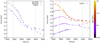 |
Fig. 1 Surface gravity log g as a functionof effective temperature Teff. Left panel: comparison of Lyon group’s BCAH98 (Baraffe et al. 1998), BHAC15 (Baraffe et al. 2015) models, and PARSEC models for [M/H] = 0 and fixed age of 5 Gyr. Right panel: PARSEC models for [M/H] = 0 and variable age from 0.01 to10 Gyr. The gray vertical lines indicate the temperature range of our PHOENIX-SESAM grid from 2900 to 4500 K. |
Uncertainties for stellar parameters for different wavelength ranges and v sin i.
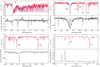 |
Fig. 2 Comparison of PHOENIX-ACES (blue) and PHOENIX-SESAM (red) models for a selection of lines. The parameters of the models are Teff = 3500 K, log g = 5.0 dex, and [Fe/H] = 0.0 dex. The models are broadened corresponding to the spectral resolution in the VIS (R ≈ 94 600) and NIR (R ≈ 80 500) channel. For each wavelength region the residual between the two models are shown. |
3.1 Models
The PHOENIX atmosphere models we used for our analysis are based on the PHOENIX code developed by Hauschildt (1992, 1993). The code has undergone continuous improvement as shown in Hauschildt et al. (1997), Hauschildt & Baron (1999), Claret et al. (2012), Husser et al. (2013). It computes one-dimensional (1D) model atmospheres for plane-parallel and spherically symmetric stars such as main sequence stars and brown dwarfs down to L and T spectral types; and white dwarfs as well as giants, including accretion disks and expanding envelopes of novae and supernovae. It can be executed in radiative transfer mode in local or non-local thermodynamic equilibrium, and synthetic spectra can be calculated in 1D or 3D. The PHOENIX code serves as a basis for several model grids of cool stars, for example, the NextGen models (Hauschildt et al. 1999); the AMES models (Allard et al. 2001) accounting for condensation and dust formation in two different approximations (AMES-dusty and AMES-cond); the BT-Settl models (Allard et al. 2011) using yet another dust approximation for very low temperature atmospheres down to the planetary mass regimes; and the PHOENIX-ACES models (Husser et al. 2013) using an updated equation of state for cool dwarfs. This last grid used a new equation of state, especially designed for molecule formation inside the coolest known stellar atmospheres.
Most recently, we calculated a new grid for temperature range between 2900 and 4500 K following Husser et al. (2013) using our latest equation of state SESAM (Meyer 2017). We used solar abundances as reported by Asplund et al. (2009), updated with values from Caffau et al. (2011), as well as updated atomic and molecular line lists. This new PHOENIX-SESAM grid was incorporated in our procedure for parameter determination. An extended grid including a detailed description will be presented ina subsequent paper. Figure 2 presents a comparison between the PHOENIX-ACES (blue) and PHOENIX-SESAM (red) models for a selection of lines. Some differences can be seen in the TiO-band (λ > 705 nm) and Ca II line (λ 866.45 nm), whereas other Ti- and Fe-lines are not significantly influenced.
3.2 Line selection
An appropriate set of spectral lines is crucial for the accurate determination of stellar parameters. Unlike studies by Raj18, who used all strong lines available in the spectra, we carefully selected the lines that we used by the following criteria. We investigated the sensitivity in Teff and metallicity of several atomic and molecular lines in the NIR by calculating the deviation between models with different parameters. For this purpose, we selected reference model spectra with Teff between 2800 K and 4000 K, [Fe/H] between –1.0 and +1.0, and with log g fixed to 5.0 for simplicity, and because we constrain this parameter from the PARSEC evolutionary models. Each reference spectrum was compared to all model spectra of the selected grid, and we calculated the deviations for each line. Then, we selected lines that showed high deviations, which is high sensitivity over a wide parameter range. As discussed in Pass18 we excluded the Ca II lines at 850.05 and 866.45 nm due to possible chromospheric emission, and the Na I doublet around 819 nm because of degeneracies in the strength and width of the lines. We also excluded some atomic and molecular lines for which the models showed shortcomings in accurately fitting the line shape.
As described above, the telluric lines in the CARMENES spectra are corrected by modeling atmospheric transmission spectra. This method, like others, suffers from imperfections due to inaccurate weather data or uncertainties in the atmospheric molecular line list. To avoid these imperfections we chose spectral lines that are not heavily affected by telluric features. Finally, yet importantly, we specifically excluded atomic lines with large Landé-factors (geff > 1.5) in the NIR and lines that are blended with lines having large Landé-factors. The factors were computed using transition parameters extracted from the current edition of the Vienna Atomic Line Database (VALD, Ryabchikova et al. 2015) or using the LS coupling approximation when this information was not available. In this way we minimized (but not completely exclude) the impact of the magnetic field on our determination of atmospheric parameters. As shown before, the Zeeman broadening scales with the square of the wavelength, so although lines in the VIS are not noticeably affected, lines with the same Landé-factors in the NIR can be broader, which might have an impact on the parameter determination. The lines of molecular species in NIR are generally very weakly magnetic sensitive or not magnetic sensitive at all, and many of them could be safely used in the analysis of atmospheric properties provided that their transition parameters are accurately known. Unfortunately, this is often not the case, as for OH (λ > 1510 nm) where we found that the models fit only poorly. The only exception is the Wing-Ford band of FeH lines around 980 nm, whose transition parameters are well known but their magnetic sensitivity is extremely high (Berdyugina & Solanki 2002; Shulyak et al. 2014), which limits using these lines in spectroscopic parameter determinations. On these grounds, we found only a few suitable lines, some of them in the NIR range, which makes them interesting for parameter determination.
Selecting spectral lines according to their magnetic sensitivity makes our analysis of NIR spectra superior to other similar works. We expect that at least one third of our sample stars have kG level magnetic fields according to their activity indicators (Schöfer et al. 2019) and we aim at minimizing possible biases in the derived stellar parameters. In Fig. 3 all lines that we used in the VIS and NIR are identified together with their Landé factors when available. Table 2 summarizes the 28 lines and molecular bands we used for parameter determination.
4 Results and discussion
We visually inspected the best fits for all stars in our sample to ensure a good fit quality and reliable stellar parameters. During this process we removed more stars from our final parameter list, because strong stellar activity or high rotational velocity led to an insufficient model fit to the spectra. Due to the fact that magnetic broadening has a larger effect on lines in the NIR range, as discussed before, we excluded more stars with parameters derived from the NIR range alone. This results in final stellar parameters derived in the VIS for 275 M dwarfs, in the NIR for 271 M dwarfs, and in VIS+NIR for 276 M dwarfs. The final sample of 282 M dwarfs is presented in Table B.1 showing the name, coordinates (Gaia DR2), spectral type (Carmencita, Caballero et al. 2016b), assumed age according to their kinematics, v sin i (Reiners et al. 2018a, if not indicated otherwise), and an activity flag. The derived parameters are listed in Table B.2 for the different wavelength ranges. In the following we compare our results derived from multiple wavelength ranges, as well as to values from the literature, and discuss outliers.
4.1 Comparison of different wavelength ranges
Figure 4 shows comparison plots for the different parameters. The upper panel presents Teff, with the stellar age color-coded. In general, the temperatures derived from the VIS and NIR wavelength ranges follow the 1:1 relation within their errors. A group of outliers is located above the 1:1 relation between 3300 K and 3600 K, showing slightly higher temperatures compared to the VIS. For temperatures higher than ~3800 K values derived from the NIR seem to be about 100–200 K lower. However, temperatures determined from VIS+NIR for the same stars almost perfectly correspond to their values in the VIS. This is shown in Fig. A.1.
Also log g (middle panel) corresponds very well in the two wavelength ranges. Young stars with ages less than 0.1 Gyr are mainly located at the lower end. Most of them have ages less than 50 Myr and are still contracting (e.g., Palla et al. 2002), which explains their lower log g. We find some trend toward lower log g values for the NIR range, where we see a group with values about 0.1–0.2 dex lower. They are related to the outlier group found in temperature, since our determination of log g depends on Teff and [Fe/H]. A clear outlier can be seen at log g 5.11 dex in the NIR. This value is about 0.5 dex higher compared to log g derived from the VIS and VIS+NIR, and belongs to J21152+257. The star also exhibits a 100 K higher temperature and 0.3 dex higher metallicity in the NIR. The deviation of its parameters might be explained by the model fit being worse in the NIR range. There are no literature values for this star, but the spectral type of M3.0 V agrees better with the temperatures derived in VIS and VIS+NIR.
The bottom panel of Fig. 4 shows the comparison in metallicity. While most stars lie on the 1:1 relation within their errorbars, there is a large group with values larger in the NIR compared to the VIS. This corresponds to what is shown in Figs. 6 and 7, where we find most of our sample to be slightly more metal-rich compared to literature.
4.2 Literature comparison
We compare our results for different wavelength ranges to literature values Maldonado et al. (2015, hereafter Mald15), RA12, GM14, Mann et al. (2015, hereafter Mann15,) and Raj2018. Teff and metallicities of Mald15 were derived using pseudo-equivalent widths in optical spectra. They used photometric relations to derive stellar masses and obtained stellar radii from empirical mass-radius relations from interferometry (Boyajian et al. 2012; von Braun et al. 2014) and eclipsing binaries (Hartman et al. 2015) to derive radii. From that they determined log g for their sample. Mann15 derived Teff by fitting BT-Settl models (Allard et al. 2013) to optical spectra. Metallicities were determined from NIR spectra using empirical relations between equivalent widths of atomic features and metallicity (Mann et al. 2013, 2014). In the latter, they obtained stellar masses using the mass-luminosity relation of Delfosse et al. (2000) and stellar radii by calculating the angular diameter from Teff and the bolometric flux, and then by using the trigonometric parallax for each star. We calculated log g for the samples of GM14 and Mann15 from the stellar masses and radii they provided. Figures 5–7 show the comparisons between our parameters in the VIS, NIR, and VIS+NIR, respectively,and literature values for the stars in common. For better readability in the figures we plotted the uncertainties of our work and of Raj18 separately in the lower right corner of each panel.
Temperatures derived by GM14 from VIS spectra are slightly higher than temperatures determined by Mann15, which are generally cooler than our results. This can be seen very well for our NIR spectra in Fig. 6 (top panel). Both authors used BT-Settl models to obtain Teff. Values fromRaj18 show a large spread of sometimes up to 300 K compared to our results. Generally, our Teff values for all wavelength ranges follow the literature very well. In log g and metallicity the plots look somewhat different. For both parameters, results from Raj18 do not correlate with our values nor with the other literature, spreading across the whole parameter range. For the other literature the plots are significantly different from the corresponding ones presented in Pass18, which can be explained by the use of different evolutionary and synthetic models, and the incorporation of different stellar ages. Concerning metallicity (bottom panels in Figs. 5–7) we find a split relation, with the majority of our values being more metal-rich than the literature. We will discuss outliers in more detail on the basis of Fig. 8 (top panel), where we include ages and activity in the plots.
Since the comparisons of VIS, NIR, and VIS+NIR follow about the same pattern in Figs. 5–7, we will focus on the values of VIS+NIR for further discussion. Due to the large spread of results from Raj18 over the whole parameter range, we will exclude them from the following analysis.
We calculated the mean absolute difference (MAD) between our results in different wavelength ranges and literature values. The results are summarized in Table 3. The highest MAD in temperature over all wavelength ranges is found for RA12. The other MADs correspond to our estimated uncertainties, some being only 10–20 K higher. For log g the MADs are at least twice as high as our uncertainties. This is different for metallicity, where MADs for VIS+NIR and VIS lie mostly within our errorbars for these wavelength ranges. In the NIR the MADs are generally higher, which can be seen as well when comparing Figs. 5 and 6, where the deviation from the 1:1 relation is larger in the NIR. Comparing MADs from Raj18 to those of other works shows much higher values, especially for log g and metallicity. Therefore, and for reference, we also calculated a total MAD excluding Raj18. In summary, it is shown that differences in the NIR for log g and metallicity are slightly higher than for VIS+NIR and VIS.
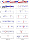 |
Fig. 3 CARMENES template spectrum of GJ 133 = J03213+799 (black) with best-fit model (blue and red). The fitting regions are marked in red. All lines are identified together with their Landé factors when available. |
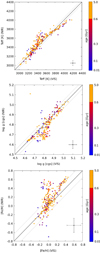 |
Fig. 4 Comparison of stellar parameters derived from VIS and NIR ranges. The assumed stellar age is color-coded. The black line indicates the 1:1 relation, the gray lines represent the 1σ deviations for VIS of 51 K, 0.04 log g, and 0.16 [Fe/H]. Error bars for VIS and NIR are plotted in the lower right corner of each plot. |
Wavelength regions and lines used for parameter determination.
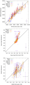 |
Fig. 5 Comparison between results from VIS and literature values for Teff (top panel), log g (middle panel), and [Fe/H] (bottom panel). The 1:1 relation is indicated by the black line. The uncertainties of this work (black) are shown in the lower right corner of each panel together with the uncertainties of Rajpurohit et al. (2018) (purple). |
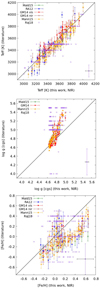 |
Fig. 6 Comparison between results from NIR and literature values for Teff (top panel), log g (middle panel), and [Fe/H] (bottom panel). The 1:1 relation is indicated by the black line. The uncertainties of this work (black) are shown in the lower right corner of each panel together with the uncertainties of Rajpurohit et al. (2018) (purple). |
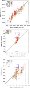 |
Fig. 7 Comparison between results from VIS+NIR and literature values for Teff (top panel), log g (middle panel), and [Fe/H] (bottom panel). The 1:1 relation is indicated by the black line. The uncertainties of this work (black) are shown in the lower right corner of each panel together with the uncertainties of Rajpurohit et al. (2018) (purple). |
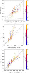 |
Fig. 8 Comparison of [Fe/H] (top panel), log g (middle panel), and Teff (bottom panel) between values of this work in VIS+NIR and literature. The age is color-coded; active star are plotted as asterisks. Outliers are identified with numbers; the green lines connect their different literature values. The black line indicates the 1:1 relation, the gray lines the 1σ deviation. |
Mean absolute difference between literature and results of this work for different wavelength ranges.
4.3 Discussion of outliers
In the following we will discuss some outliers from Fig. 7, mainly considering metallicity and log g. Figure 8 shows the same plots as Fig. 7, with the estimated age of the stars color-coded. Additionally, active stars are plotted as asterisks. We define a star to be active if the Hα pseudo-equivalent width is less than –0.3 Å as described in Schöfer et al. (2019), or if the star shows Ca II emission (see Pass18). Active stars are identified in Table B.1 with an activity flag 1. Furthermore, we define outliers if our value deviates by more than our estimated uncertainties from the literature values. For guidance, these 1σ deviations are plotted as gray lines.
First, we point out general trends seen in the plots. As mentioned above, the metallicity comparison shows a split correlation. In the top panel of Fig. 8 we see that mainly stars located below the 1:1 relation have values deviating more than 1σ. Most active stars correspond very well to literature values, which supports our method of line selection since we found this parameter to be most influenced by activity.
In log g (Fig. 8, middle panel) we find several young stars with lower values compared to literature. As explained above, they might still be contracting due to their young age of less than 50 Myr. Even though we carefully selected magnetically less sensitive lines, there are several stars in our sample that are considerably active, and therefore also less sensitive lines are affected. For metallicity (Fig. 8, top panel) all but a few of these star values coincide with the literature. However, in log g we can see them clearly as outliers at the upper end of the plot. They represent values mainly determined from masses and radii derived by Mann15. The same offset was also found by Schw19 for log g > 5.0. Additionally, we see many stars located above the 1:1 relation, meaning smaller log g compared to those from the literature. This might be explained by the use of the PARSEC evolutionary models, which provide smaller values than the Baraffe models used in Pass18 and Schw19. In the bottom panel of Fig. 8 a small group of outliers at the cool end is represented by results from RA12 and Mann15, and was also found by Pass18. In addition we find these stars to be active.
In the following discussion we will not include active stars and stars younger than 5 Gyr. For some stars our values derived from VIS, NIR, and VIS+NIR coincide within their errors, however they deviate by more than 1σ from literature values. Their fits and spectra are of good or very good quality, therefore we are very confident of our resulting parameters and cannot find any explanation for their deviation from the literature. For this reason, these stars are not identified with a number and not considered as outliers. For stars with multiple literature values, we consider only those for which all literature values deviate more than 1σ from our value to be outliers. For identification we connect these points using a green line. Also all stars listed in the following have very good quality spectra and fits in all wavelength ranges, unless stated otherwise.
(1) J12248-182, (2) J23492+024, (3) J11033+359
These stars appear more metal-poor in the NIR than in the VIS and VIS+NIR ranges. The NIR values coincide with literature values within 1σ. Teff obtained from all three wavelength ranges agree with each other. Schw19 speculated if (1) was a subdwarf and therefore labeled it an outlier. (3) was also claimed to be an outlier in Schw19 due to a mismatch of photometric and interferometric radii. All three stars might be members of the thick disk according to their kinematics and therefore more than 5 Gyrs old.
(4) J16581+257
The VIS metallicity of this star is lower than those derived from NIR and VIS+NIR. However, with a value of +0.17 dex it is still higher than literature values from RA12 (–0.04 dex) and Mann15 (+0.03 dex). At this point we cannot explain the differences between our values and the literature.
(5) J17578+046 (Barnard’s star)
Since Barnard’s star is claimed to be old (7–10 Gyr Ribas et al. 2018), we assumed an age of 8 Gyr, using older evolutionary models resulting in smaller log g. However, the final stellar parameters do not change significantly compared to the 5 Gyr model. Teff and metallicities in all wavelength ranges coincide within their errors, but the metallicity seems to be a bit too high compared to the literature. Because the measurement of RA12 lies within 1σ, the star is not considered an outlier in metallicity. Assuming a more metal-poor value would translate into a ~0.1 dex higher log g, which would still be considerably smaller than literature values.
(6) J11509+483
Although the quality of the spectrum and the fit for this star is moderate, the temperatures and metallicities obtained from different wavelength ranges coincide and are comparable with the literature (Mann15). One explanation for the deviation in log g (see Fig. 8, middle panel) might be that Mann15 determined too low of a stellar mass from the mass-luminosity relation (Delfosse et al. 2000), which results in too high of a log g. Using an updated mass-luminosity relation (Mann et al. 2019) Schw19 derived a slightly higher mass for this star. This would lead to a lower, but still too high log g, which makes it more likely that the reason lies in the use of PARSEC models, where all log g values tend to be slightly smaller.
(7) J11477+008
For this star there are literature values from Mald15, RA12, GM14, and Mann15. The star appears as an outlier only in log g, where we measure values about 0.1–0.3 dex smaller than in the literature. Our metallicity values in all wavelength ranges agree with the literature within their errors. RA12 measured a temperature about 200 K cooler (3065 K), whereas Mald15 determined a value of about 100 K hotter (3382 K). The other measurements agree very well with ours in all wavelength ranges.
(8) J22115+184
Schw19 derived an almost 200 K cooler temperature for this star, as well as a considerably lower metallicity (–0.13 dex). GM14 measured a temperature and metallicity of 3653 K and +0.26 dex, which both agree with our values from the VIS and VIS+NIR. In the NIR we measure a slightly higher temperature and considerably higher metallicity of +0.58 dex. Since the spectrum and the fit are of very good quality, both in the VIS and NIR, we cannot pin down the reason for this discrepancy.
(9) J22503-070, (11) J04290+219, (12) J05127+196
For these stars temperatures measured from the NIR correspond better to the literature, however they all lie within 100 K.
(10) J02222+478
Literature values for this star are controversial, with 4058 K derived by GM14 and 3785 K obtained by Mann15. In the NIR we measured a temperature of 3840 K, which is about 100 K cooler than in VIS+NIR. However, our derived values lie well between the literature values, which is why we consider them as good measurements.
5 Summary
The CARMENES instrument at Calar Alto Observatory performs high-accuracy radial velocity measurements in the VIS and NIR wavelength range simultaneously. We used the high-S/N template spectrum for each CARMENES sample M-dwarf to derive photospheric stellar parameters in the VIS, NIR, and VIS+NIR wavelength ranges for 282 stars. We calculated a new grid of PHOENIX model atmospheres incorporating a new equation of state, and new atomic and molecular line lists. Additionally, we carefully selected lines in the NIR that are sensitive to changes in stellar parameters, but insensitive to Zeeman-broadening caused by magnetic activity. Stellar activity is a crucial stellar property, influencing line profiles, which other studies did not consider. Furthermore, we involved different evolutionary models for deriving log g to account for stellar ages younger than 5 Gyr.
For thefirst time we directly compared stellar parameters such as Teff, log g, and [Fe/H] determined from multiple wavelength ranges simultaneously. There we find that Teff is mainly consistent over all wavelength ranges, although we find a little larger offset in the NIR. This might be because the TiO-bands in the VIS are a very strong indicator for temperature. A direct comparison of log g shows that this parameter also corresponds very well in all wavelength ranges. A trend toward lower log g in the NIR canbe found compared to values derived for the same stars in the VIS and VIS+NIR. Because the determination of log g depends on Teff and metallicity, an explanation for that might be found in the metallicity. For this property we see a clear trend toward more metal-rich values in the NIR than in the VIS. Also some values in VIS+NIR are slightly higher, which indicates a rise in metallicity toward longer wavelengths. Since metallicity is a basic property of the star and therefore wavelength independent, the cause for this most probably lies in the determination method or the synthetic models. Fitting synthetic spectra to derive stellar parameters has already been used in several studies (e.g., Gaidos & Mann 2014; Lindgren & Heiter 2017; Passegger et al. 2016, 2018; Rajpurohit et al. 2018). While the fitting process itself is less crucial for the final result, the use of different synthetic model grids could lead to significant differences. However, a discussion on this topic is beyond the scope of this work.
As mentioned by other works before (e.g., Passegger et al. 2016, 2018) synthetic model spectra considerably improved over the last years, however they still suffer from some deficiencies. In the VIS, these shortcomings have been pointed out by Passegger et al. (2018), concerning Ti I (λ 846.9 and 867.77 nm) and Fe I (λ 867.71 and 882.6 nm). In the NIR we find similar deficiencies in the K I lines where the models cannot fit the line cores. Moreover, due to the different spatial radial velocity and heliocentric correction for each star, the Fe I line at λ 1112.3 nm is for some stars contaminated by telluric lines and therefore cannot be used.
Comparisons of our derived parameters to literature values shows good agreement for the effective temperature. Although most of our values are consistent with the literature in log g and metallicity, there is a trend toward lower log g (most likely due to the use of PARSEC evolutionary models) and higher metallicity. As for now we cannot be absolutely certain about the reason for finding more metal-rich values in the NIR. Results from Rajpurohit et al. (2018) exhibit a large spread over the whole parameter range, with high deviations of up to 400 K in temperature and 1.0 dex in log g and metallicity compared to our work. We cannot find any correlations with our values or other literature. The overall distribution of the Rajpurohit et al. (2018) parameters is similar to what we found in early studies on stellar parameter determination by leaving log g as a free fit parameter. That method might reduce biases in the parameter space, but it also is more susceptible to degeneracies between the parameters, especially log g and metallicity, as described in Passegger et al. (2018).
Precise determination of the metallicity is still a challenging task. Different methods and synthetic models can lead to different results. In the literature we sometimes find very diverse measurements for the same star (e.g., GJ 205: 0.0 Maldonado et al. 2015, +0.49 Mann et al. 2015). Our comparison of stellar parameters determined from multiple wavelength ranges shows that deviations from the literature are smallest for the VIS, followed by the VIS+NIR, and highest in the NIR, especially concerning metallicity. This might be explained by continuing shortcomings in synthetic models and the lower number of useful and parameter-sensitive lines in the NIR compared to the VIS. However, the differences between VIS and VIS+NIR are marginal. For that reason, we emphasize the use of both ranges for parameter determination in order to maximize the amount of spectral information available and minimize possible effects caused by imperfect modeling.
Acknowledgements
We thank an anonymous referee for helpful comments that improved the quality of this paper. CARMENES is an instrument for the Centro Astronómico Hispano-Alemń de Calar Alto (CAHA, Almería, Spain). CARMENES is funded by the German Max-Planck-Gesellschaft (MPG), the Spanish Consejo Superior de Investigaciones Científicas (CSIC), the European Union through FEDER/ERF FICTS-2011-02 funds, and the members of the CARMENES Consortium (Max- Planck-Institut für Astronomie, Instituto de Astrofísica de Andalucía, Landessternwarte Königstuhl, Institut de Ciències de l’Espai, Insitut für Astrophysik Göttingen, Universidad Complutense de Madrid, Thüringer Landessternwarte Tautenburg, Instituto de Astrofísica de Canarias, Hamburger Sternwarte, Centro de Astrobiología, and Centro Astronómico Hispano- Alemán), with additional contributions by the Spanish Ministry of Economy, the German Science Foundation through the Major Research Instrumentation Programme, and DFG Research Unit FOR2544 “Blue Planets around Red Stars”, the Klaus Tschira Stiftung, the states of Baden-Württemberg and Niedersachsen, and by the Junta de Andalucía. This work is based on data from the CARMENES data archive at CAB (INTA-CSIC). We acknowledge financial support from the Agencia Estatal de Investigación of the Ministerio de Ciencia, Innovación y Universidades, and the European FEDER/ERF funds through projects AYA2018-84089, ESP2017-87676-C5-1-R, ESP2016-80435-C2-1-R, AYA2016-79425-C3-1/2/3-P, AYA2015-69350-C3-2-P, and the Centre of Excellence “Severo Ochoa” and “María de Maeztu” awards to the Instituto de Astrofísica de Canarias (SEV-2015-0548), Instituto de Astrofísica de Andalucía (SEV-2017-0709), and Centro de Astrobiología (MDM-2017-0737), and the Generalitat de Catalunya/CERCA programme. Some of the calculations presented here were performed at the RRZ of the Universität Hamburg, at the Höchstleistungs Rechenzentrum Nord (HLRN), and at the National Energy Research Supercomputer Center (NERSC), which is supported by the Office of Science of the U.S. Department of Energy under Contract No. DE-AC03-76SF00098. We thank all these institutions for a generous allocation of computer time. P.H.H. gratefully acknowledges the support of NVIDIA Corporation with the donation of a Quadro P6000 GPU used in this research. This work has made use of the VALD database, operated at Uppsala University, the Institute of Astronomy RAS in Moscow, and the University of Vienna. This work has made use of data from the European Space Agency (ESA) mission Gaia (https://www.cosmos.esa.int/gaia), processed by the Gaia Data Processing and Analysis Consortium (DPAC, https://www.cosmos.esa.int/web/gaia/dpac/consortium). Funding for the DPAC has been provided by national institutions, in particular the institutions participating in the Gaia Multilateral Agreement.
Appendix A Additional figures
Figure A.1 presents the same comparison plots as in Fig. 4, including values for the combined wavelength ranges VIS+NIR. The behavior of the NIR values compared to VIS+NIR is very similar to what was already shown in Fig. 4, where we compared the NIR with the VIS results. A small group of outliers from the VIS is found between 3600 and 3800 K that exhibit about 200 K cooler temperatures compared to the NIR and VIS+NIR. About half of them have ages younger than 0.15 Gyr. The same stars are also outliers in log g (middle panel) and metallicity (bottom panel).
For log g (middle panel) it is shown that most values coincide very well over all wavelength ranges. The small group of outliers in the VIS can be found with log g of about 0.1–0.2 dex higher compared to the NIR and VIS+NIR.
The comparison in metallicity is presented in the bottom panel of Fig. A.1. The VIS outlier group exhibits up to 0.4 dex lower metallicities compared to VIS+NIR, whereas values for other stars perfectly agree in VIS and VIS+NIR. We will discuss the properties of the VIS outlier group in more detail in the following.
The VIS outlier group
This group consists of nine stars, for which we derive cooler Teff, larger log g, and lower metallicities compared to the NIR and VIS+NIR. Hence, their parameters in the latter two wavelength ranges agree with each other within 1σ. Four of these stars are younger than 0.15 Gyr and two are magnetically active (identified with an asterisk in Fig. A.1). However, all fits to the spectra in either wavelength range are of good or very good quality, which cannot explain the deviations in the parameters. For two stars, which we marked with letters a and b, there are literature values available.
- (a)
J02358+202: literature values for Teff and log g from Mann15 perfectly agree with our VIS values, however, they measured a metallicity of +0.12 dex, which lies between our values for VIS (–0.15 dex) and VIS+NIR (+0.38 dex). The estimated age for this star is 0.1 Gyr.
- (b)
J04429+189: for this star there are four different literature references from Mald15, RA12, GM14, and Mann15. Temperatures are spread between 3581 K (RA12) and 3721 K (GM14). Metallicities range from +0.03 dex (Mald15) and +0.14 dex (GM14, Mann15) and lie between our measurements in the VIS (–0.08 dex) and VIS+NIR (+0.33 dex).
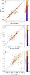 |
Fig. A.1 Comparison of stellar parameters derived from different wavelength ranges. Values from VIS+NIR are plotted on the x-axis, values for VIS (filled circles) and NIR (open squares) are shown on the y-axis with the age color-coded. The black line indicates the 1:1 relation, the gray lines represent the 1σ deviations for VIS+NIR of 54 K, 0.06 log g, and 0.19 [Fe/H]. |
Appendix B Additional tables
Tables B.1 and B.2 are available in their entirety in a machine-readable form at the CDS. An excerpt is shown here for guidance regarding their form and content.
CARMENES sample stars investigated in this work.
Basic astrophysical parameters of investigated stars for different wavelength regimes.
References
- Allard, F., Hauschildt, P. H., Alexander, D. R., Tamanai, A., & Schweitzer, A. 2001, ApJ, 556, 357 [NASA ADS] [CrossRef] [Google Scholar]
- Allard, F., Homeier, D., & Freytag, B. 2011, in 16th Cambridge Workshop on Cool Stars, Stellar Systems, and the Sun, eds. C. Johns-Krull, M. K. Browning, & A. A. West, ASP Conf. Ser., 448, 91 [NASA ADS] [Google Scholar]
- Allard, F., Homeier, D., & Freytag, B. 2012, Phil. Trans. R. Soc. London, Ser. A, 370, 2765 [Google Scholar]
- Allard, F., Homeier, D., Freytag, B., et al. 2013, Mem. Soc. Astron. It. Supp., 24, 128 [Google Scholar]
- Asplund, M., Grevesse, N., Sauval, A. J., & Scott, P. 2009, ARA&A, 47, 481 [NASA ADS] [CrossRef] [Google Scholar]
- Baraffe, I., Chabrier, G., Allard, F., & Hauschildt, P. H. 1998, A&A, 337, 403 [NASA ADS] [Google Scholar]
- Baraffe, I., Homeier, D., Allard, F., & Chabrier, G. 2015, A&A, 577, A42 [NASA ADS] [CrossRef] [EDP Sciences] [Google Scholar]
- Baroch, D., Morales, J. C., Ribas, I., et al. 2018, A&A, 619, A32 [NASA ADS] [CrossRef] [EDP Sciences] [Google Scholar]
- Bauer, F. F., Zechmeister, M., & Reiners, A. 2015, A&A, 581, A117 [NASA ADS] [CrossRef] [EDP Sciences] [Google Scholar]
- Berdyugina, S. V., & Solanki, S. K. 2002, A&A, 385, 701 [NASA ADS] [CrossRef] [EDP Sciences] [Google Scholar]
- Birky, J. L., Aganze, C., Burgasser, A. J., et al. 2017, Am. Astron. Soc. Meet. Abstr., 229, 240 [Google Scholar]
- Boyajian, T. S., von Braun, K., van Belle, G., et al. 2012, ApJ, 757, 112 [NASA ADS] [CrossRef] [Google Scholar]
- Bressan, A., Marigo, P., Girardi, L., et al. 2012, MNRAS, 427, 127 [NASA ADS] [CrossRef] [Google Scholar]
- Caballero, J. A., Guàrdia, J., López del Fresno, M., et al. 2016a, Proc. SPIE, 9910, 99100E [Google Scholar]
- Caballero, J. A., Cortés-Contreras, M., Alonso-Floriano, F. J., et al. 2016b, 19th Cambridge Workshop on Cool Stars, Stellar Systems,and the Sun (Berlin: Springer), 148 [Google Scholar]
- Caffau, E., Ludwig, H.-G., Steffen, M., Freytag, B., & Bonifacio, P. 2011, Sol. Phys., 268, 255 [NASA ADS] [CrossRef] [Google Scholar]
- Chen, Y., Girardi, L., Bressan, A., et al. 2014, MNRAS, 444, 2525 [NASA ADS] [CrossRef] [Google Scholar]
- Chen, Y., Bressan, A., Girardi, L., et al. 2015, MNRAS, 452, 1068 [NASA ADS] [CrossRef] [Google Scholar]
- Claret, A., Hauschildt, P. H., & Witte, S. 2012, A&A, 546, A14 [NASA ADS] [CrossRef] [EDP Sciences] [Google Scholar]
- Cortés-Contreras, M. 2016, PhD Thesis, Universidad Complutense de Madrid, Spain [Google Scholar]
- Delfosse, X., Forveille, T., Ségransan, D., et al. 2000, A&A, 364, 217 [NASA ADS] [Google Scholar]
- Gaia Collaboration (Prusti, T., et al.) 2016, A&A, 595, A1 [NASA ADS] [CrossRef] [EDP Sciences] [Google Scholar]
- Gaia Collaboration (Brown, A. G. A., et al.) 2018, A&A, 616, A1 [NASA ADS] [CrossRef] [EDP Sciences] [Google Scholar]
- Gaidos, E., & Mann, A. W. 2014, ApJ, 791, 54 [NASA ADS] [CrossRef] [Google Scholar]
- Gordon, I. E., Rothman, L. S., Hill, C., et al. 2017, J. Quant. Spectr. Rad. Transf., 203, 3 [Google Scholar]
- Hartman, J. D., Bayliss, D., Brahm, R., et al. 2015, AJ, 149, 166 [NASA ADS] [CrossRef] [Google Scholar]
- Hauschildt, P. H. 1992, J. Quant. Spectr. Rad. Transf., 47, 433 [Google Scholar]
- Hauschildt, P. H. 1993, J. Quant. Spectr. Rad. Transf., 50, 301 [Google Scholar]
- Hauschildt, P. H., & Baron, E. 1999, J. Comput. Appl. Math., 109, 41 [NASA ADS] [CrossRef] [Google Scholar]
- Hauschildt, P. H., Baron, E., & Allard, F. 1997, ApJ, 483, 390 [NASA ADS] [CrossRef] [Google Scholar]
- Hauschildt, P. H., Allard, F., & Baron, E. 1999, ApJ, 512, 377 [NASA ADS] [CrossRef] [Google Scholar]
- Husser, T.-O., Wende-von Berg, S., Dreizler, S., et al. 2013, A&A, 553, A6 [NASA ADS] [CrossRef] [EDP Sciences] [Google Scholar]
- Kaminski, A., Trifonov, T., Caballero, J. A., et al. 2018, A&A, 618, A115 [NASA ADS] [CrossRef] [EDP Sciences] [Google Scholar]
- Kausch, W., Noll, S., Smette, A., et al. 2014, ASP Conf. Ser., 485, 403 [NASA ADS] [Google Scholar]
- Landi Degl’Innocenti, E., & Landolfi, M. 2004, Astrophys. Space Sci. Lib., 307 [Google Scholar]
- Lindgren, S., & Heiter, U. 2017, A&A, 604, A97 [NASA ADS] [CrossRef] [EDP Sciences] [Google Scholar]
- Luque, R., Nowak, G., Pallé, E., et al. 2018, A&A, 620, A171 [NASA ADS] [CrossRef] [EDP Sciences] [Google Scholar]
- Maldonado, J., Affer, L., Micela, G., et al. 2015, A&A, 577, A132 [NASA ADS] [CrossRef] [EDP Sciences] [Google Scholar]
- Mann, A. W., Brewer, J. M., Gaidos, E., Lépine, S., & Hilton, E. J. 2013, AJ, 145, 52 [NASA ADS] [CrossRef] [Google Scholar]
- Mann, A. W., Deacon, N. R., Gaidos, E., et al. 2014, AJ, 147, 160 [NASA ADS] [CrossRef] [Google Scholar]
- Mann, A. W., Feiden, G. A., Gaidos, E., Boyajian, T., & von Braun, K. 2015, ApJ, 804, 64 [NASA ADS] [CrossRef] [Google Scholar]
- Mann, A. W., Dupuy, T., Kraus, A. L., et al. 2019, ApJ, 871, 63 [NASA ADS] [CrossRef] [Google Scholar]
- Martínez-Rodríguez, H. 2014, PhD Thesis, Universidad Complutense de Madrid, Spain [Google Scholar]
- Meyer, M. 2017, PhD Thesis, Universität Hamburg, Germany [Google Scholar]
- Montes, D., López-Santiago, J., Fernández-Figueroa, M. J., & Gálvez, M. C. 2001, A&A, 379, 976 [NASA ADS] [CrossRef] [EDP Sciences] [Google Scholar]
- Nagel, E., Czesla, S., Schmitt, J. H. M. M., et al. 2019, A&A, 622, A153 [NASA ADS] [CrossRef] [EDP Sciences] [Google Scholar]
- Newton, E. R., Charbonneau, D., Irwin, J., et al. 2014, AJ, 147, 20 [NASA ADS] [CrossRef] [Google Scholar]
- Palla, F., Zinnecker, H., Maeder, A., & Meynet, G., eds. 2002, Physics of star formation in galaxies (Berlin: Springer-Verlag) [CrossRef] [Google Scholar]
- Passegger, V. M. 2017, PhD Thesis, Georg-August-Universität Göttingen, Germany [Google Scholar]
- Passegger, V. M., Wende-von Berg, S., & Reiners, A. 2016, A&A, 587, A19 [NASA ADS] [CrossRef] [EDP Sciences] [Google Scholar]
- Passegger, V. M., Reiners, A., Jeffers, S. V., et al. 2018, A&A, 615, A6 [NASA ADS] [CrossRef] [EDP Sciences] [Google Scholar]
- Piskunov, N. E., & Valenti, J. A. 2002, A&A, 385, 1095 [NASA ADS] [CrossRef] [EDP Sciences] [Google Scholar]
- Quirrenbach, A., Amado, P. J., Ribas, I., et al. 2018, SPIE Conf. Ser., 10702, 107020W [Google Scholar]
- Rajpurohit, A. S., Allard, F., Rajpurohit, S., et al. 2018, A&A, 620, A180 [NASA ADS] [CrossRef] [EDP Sciences] [Google Scholar]
- Reiners, A., Basri, G., & Browning, M. 2009, ApJ, 692, 538 [NASA ADS] [CrossRef] [Google Scholar]
- Reiners, A., Zechmeister, M., Caballero, J. A., et al. 2018a, A&A, 612, A49 [NASA ADS] [CrossRef] [EDP Sciences] [Google Scholar]
- Reiners, A., Ribas, I., Zechmeister, M., et al. 2018b, A&A, 609, L5 [Google Scholar]
- Ribas, I., Tuomi, M., Reiners, A., et al. 2018, Nature, 563, 365 [NASA ADS] [CrossRef] [Google Scholar]
- Rodríguez Martínez, R., Ballard, S., Mayo, A., et al. 2018, ArXiv e-prints [arXiv:1808.03652] [Google Scholar]
- Rojas-Ayala, B., Covey, K. R., Muirhead, P. S., & Lloyd, J. P. 2012, ApJ, 748, 93 [NASA ADS] [CrossRef] [Google Scholar]
- Ryabchikova, T., Piskunov, N., Kurucz, R. L., et al. 2015, Phys. Scr, 90, 054005 [NASA ADS] [CrossRef] [Google Scholar]
- Sarkis, P., Henning, T., Kürster, M., et al. 2018, AJ, 155, 257 [NASA ADS] [CrossRef] [Google Scholar]
- Schäfer, S., Guenther, E. W., Reiners, A., et al. 2018, SPIE Conf. Ser., 10702, 1070276 [Google Scholar]
- Schöfer, P., Jeffers, S. V., Reiners, A., et al. 2019, A&A, 623, A44 [NASA ADS] [CrossRef] [EDP Sciences] [Google Scholar]
- Schweitzer, A., Passegger, V. M., Cifuentes, C., et al. 2019, A&A, 625, A68 [NASA ADS] [CrossRef] [EDP Sciences] [Google Scholar]
- Shulyak, D., Reiners, A., Seemann, U., Kochukhov, O., & Piskunov, N. 2014, A&A, 563, A35 [NASA ADS] [CrossRef] [EDP Sciences] [Google Scholar]
- Shulyak, D., Reiners, A., Engeln, A., et al. 2017, Nat. Astron., 1, 0184 [NASA ADS] [CrossRef] [Google Scholar]
- Smette, A., Sana, H., Noll, S., et al. 2015, A&A, 576, A77 [NASA ADS] [CrossRef] [EDP Sciences] [Google Scholar]
- Sneden, C. 1973, ApJ, 184, 839 [NASA ADS] [CrossRef] [Google Scholar]
- Sneden, C., Bean, J., Ivans, I., Lucatello, S., & Sobeck, J. 2012, Astrophysics Source Code Library [record ascl:1202.009] [Google Scholar]
- Souto, D., Cunha, K., García-Hernández, D. A., et al. 2017, ApJ, 835, 239 [NASA ADS] [CrossRef] [Google Scholar]
- Souto, D., Unterborn, C. T., Smith, V. V., et al. 2018, ApJ, 860, L15 [NASA ADS] [CrossRef] [Google Scholar]
- Tang, J., Bressan, A., Rosenfield, P., et al. 2014, MNRAS, 445, 4287 [NASA ADS] [CrossRef] [Google Scholar]
- Trifonov, T., Kürster, M., Zechmeister, M., et al. 2018, A&A, 609, A117 [NASA ADS] [CrossRef] [EDP Sciences] [Google Scholar]
- Valenti, J. A., & Piskunov, N. 2012, Astrophysics Source Code Library [record ascl:1202.013] [Google Scholar]
- Veyette, M. J., & Muirhead, P. S. 2018, ApJ, 863, 166 [NASA ADS] [CrossRef] [Google Scholar]
- Veyette, M. J., Muirhead, P. S., Mann, A. W., et al. 2017, ApJ, 851, 26 [NASA ADS] [CrossRef] [Google Scholar]
- von Braun K., Boyajian, T. S., van Belle, G. T., et al. 2014, MNRAS, 438, 2413 [NASA ADS] [CrossRef] [Google Scholar]
- Wright, J. T., & Eastman, J. D. 2014, PASP, 126, 838 [NASA ADS] [CrossRef] [EDP Sciences] [Google Scholar]
- Zechmeister, M., Kürster, M., & Endl, M. 2009, A&A, 505, 859 [NASA ADS] [CrossRef] [EDP Sciences] [Google Scholar]
- Zechmeister, M., Anglada-Escudé, G., & Reiners, A. 2014, A&A, 561, A59 [NASA ADS] [CrossRef] [EDP Sciences] [Google Scholar]
- Zechmeister, M., Reiners, A., Amado, P. J., et al. 2018, A&A, 609, A12 [CrossRef] [Google Scholar]
- Zechmeister, M., Dreizler, S., Ribas, I., Reiners, A., & Caballero, J. A. 2019, A&A, 627, A49 [NASA ADS] [EDP Sciences] [Google Scholar]
All Tables
Uncertainties for stellar parameters for different wavelength ranges and v sin i.
Mean absolute difference between literature and results of this work for different wavelength ranges.
Basic astrophysical parameters of investigated stars for different wavelength regimes.
All Figures
|
Fig. 1 Surface gravity log g as a functionof effective temperature Teff. Left panel: comparison of Lyon group’s BCAH98 (Baraffe et al. 1998), BHAC15 (Baraffe et al. 2015) models, and PARSEC models for [M/H] = 0 and fixed age of 5 Gyr. Right panel: PARSEC models for [M/H] = 0 and variable age from 0.01 to10 Gyr. The gray vertical lines indicate the temperature range of our PHOENIX-SESAM grid from 2900 to 4500 K. |
| In the text | |
|
Fig. 2 Comparison of PHOENIX-ACES (blue) and PHOENIX-SESAM (red) models for a selection of lines. The parameters of the models are Teff = 3500 K, log g = 5.0 dex, and [Fe/H] = 0.0 dex. The models are broadened corresponding to the spectral resolution in the VIS (R ≈ 94 600) and NIR (R ≈ 80 500) channel. For each wavelength region the residual between the two models are shown. |
| In the text | |
|
Fig. 3 CARMENES template spectrum of GJ 133 = J03213+799 (black) with best-fit model (blue and red). The fitting regions are marked in red. All lines are identified together with their Landé factors when available. |
| In the text | |
|
Fig. 4 Comparison of stellar parameters derived from VIS and NIR ranges. The assumed stellar age is color-coded. The black line indicates the 1:1 relation, the gray lines represent the 1σ deviations for VIS of 51 K, 0.04 log g, and 0.16 [Fe/H]. Error bars for VIS and NIR are plotted in the lower right corner of each plot. |
| In the text | |
|
Fig. 5 Comparison between results from VIS and literature values for Teff (top panel), log g (middle panel), and [Fe/H] (bottom panel). The 1:1 relation is indicated by the black line. The uncertainties of this work (black) are shown in the lower right corner of each panel together with the uncertainties of Rajpurohit et al. (2018) (purple). |
| In the text | |
|
Fig. 6 Comparison between results from NIR and literature values for Teff (top panel), log g (middle panel), and [Fe/H] (bottom panel). The 1:1 relation is indicated by the black line. The uncertainties of this work (black) are shown in the lower right corner of each panel together with the uncertainties of Rajpurohit et al. (2018) (purple). |
| In the text | |
|
Fig. 7 Comparison between results from VIS+NIR and literature values for Teff (top panel), log g (middle panel), and [Fe/H] (bottom panel). The 1:1 relation is indicated by the black line. The uncertainties of this work (black) are shown in the lower right corner of each panel together with the uncertainties of Rajpurohit et al. (2018) (purple). |
| In the text | |
|
Fig. 8 Comparison of [Fe/H] (top panel), log g (middle panel), and Teff (bottom panel) between values of this work in VIS+NIR and literature. The age is color-coded; active star are plotted as asterisks. Outliers are identified with numbers; the green lines connect their different literature values. The black line indicates the 1:1 relation, the gray lines the 1σ deviation. |
| In the text | |
|
Fig. A.1 Comparison of stellar parameters derived from different wavelength ranges. Values from VIS+NIR are plotted on the x-axis, values for VIS (filled circles) and NIR (open squares) are shown on the y-axis with the age color-coded. The black line indicates the 1:1 relation, the gray lines represent the 1σ deviations for VIS+NIR of 54 K, 0.06 log g, and 0.19 [Fe/H]. |
| In the text | |
Current usage metrics show cumulative count of Article Views (full-text article views including HTML views, PDF and ePub downloads, according to the available data) and Abstracts Views on Vision4Press platform.
Data correspond to usage on the plateform after 2015. The current usage metrics is available 48-96 hours after online publication and is updated daily on week days.
Initial download of the metrics may take a while.