| Issue |
A&A
Volume 627, July 2019
|
|
|---|---|---|
| Article Number | A9 | |
| Number of page(s) | 9 | |
| Section | The Sun | |
| DOI | https://doi.org/10.1051/0004-6361/201834125 | |
| Published online | 25 June 2019 | |
Comparing extrapolations of the coronal magnetic field structure at 2.5 R⊙ with multi-viewpoint coronagraphic observations
1
INAF-Osservatorio Astronomico di Capodimonte, Salita Moiariello 16, 80131 Napoli, Italy
e-mail: csasso@oacn.inaf.it
2
Institut de Recherche en Astrophysique et Planétologie, University of Toulouse, CNRS, UPS, CNES, 9 Avenue Colonel Roche, BP 44346, 31028 Toulouse Cedex 4A, France
3
Space Science Division, US Naval Research Laboratory, Washington, DC, USA
4
Johns Hopkins University Applied Physics Laboratory, Laurel, MD, USA
5
INAF-Turin Astrophysical Observatory, Via Osservatorio 20, 10025 Pino Torinese (TO), Italy
6
INAF-Catania Astrophysical Observatory, Via Santa Sofia 78, 95123 Catania, Italy
7
CNR-Institute of Photonics and Nanotechnologies, Via Trasea 7, 35131 Padova, Italy
8
INAF-Arcetri Astrophysical Observatory, Largo Enrico Fermi 5, 50125 Firenze, Italy
9
University of Padova, Department of Physics and Astronomy “Galileo Galilei”, Via Marzolo, 8, 35131 Padova, Italy
10
University of Florence, Dept. of Physics and Astronomy, Largo Enrico Fermi 2, 50125 Firenze, Italy
Received:
23
August
2018
Accepted:
20
May
2019
The magnetic field shapes the structure of the solar corona, but we still know little about the interrelationships between the coronal magnetic field configurations and the resulting quasi-stationary structures observed in coronagraphic images (such as streamers, plumes, and coronal holes). One way to obtain information on the large-scale structure of the coronal magnetic field is to extrapolate it from photospheric data and compare the results with coronagraphic images. Our aim is to verify whether this comparison can be a fast method to systematically determine the reliability of the many methods that are available for modeling the coronal magnetic field. Coronal fields are usually extrapolated from photospheric measurements that are typically obtained in a region close to the central meridian on the solar disk and are then compared with coronagraphic images at the limbs, acquired at least seven days before or after to account for solar rotation. This implicitly assumes that no significant changes occurred in the corona during that period. In this work, we combine images from three coronagraphs (SOHO/LASCO-C2 and the two STEREO/SECCHI-COR1) that observe the Sun from different viewing angles to build Carrington maps that cover the entire corona to reduce the effect of temporal evolution to about five days. We then compare the position of the observed streamers in these Carrington maps with that of the neutral lines obtained from four different magnetic field extrapolations to evaluate the performances of the latter in the solar corona. Our results show that the location of coronal streamers can provide important indications to distinguish between different magnetic field extrapolations.
Key words: Sun: corona / Sun: heliosphere / Sun: magnetic fields
© ESO 2019
1. Introduction
It is well-known that the magnetic field of the Sun drives the dynamics and structure of the solar corona. Eclipses and coronagraphic images reveal that the plasma in the corona is organized in long-lived structures, such as streamers, coronal holes, and plumes, which follow the configuration of the large-scale magnetic field. However, the details of the interplay between plasma and magnetic field are often hard to establish. One way to obtain information on the large-scale structure of the coronal magnetic field is to extrapolate it from photospheric data and compare the results with coronagraphic images. Usually these extrapolations are based on photospheric field measurements that are acquired in a region close to the central meridian on the solar disk and are then compared with coronal structures that are observed above the limbs. Nevertheless, this comparison requires the assumption that no significant changes occurred in the global distribution of large-scale features in the solar corona for about seven days to account for one quarter of solar rotation.
The purpose of this work is to show how coronagraphic white-light images might provide (or fail to do so) additional boundary conditions for the extrapolated fields. This determination is particularly important for space missions, for which the connectivity problem is crucial. Quick but reliable checks like the one that we discuss here will help observation planning, even with relatively little data (i.e., “low-latency data” or “beacon”) and short computational time. The work described here was indeed part of the activities performed for the Modeling and Data Analysis Working Group (MADAWG), which aims to optimize the coronal magnetic field extrapolations to establish the magnetic connectivity of the Solar Orbiter spacecraft (Müller & Marsden 2013) with the Sun, to relate future remote-sensing and in situ observations. Alternative and more sophisticated methods such as tomography would of course provide a more complete view of the distribution of the white-light features. We need, however, to minimize the computational time and the amount of data that is to be analyzed routinely (on a daily basis).
It has long been recognized that the streamers seen in white-light coronagraphic images represent edgewise views of the coronal plasma surrounding the coronal current sheet, which rotates with the Sun (e.g., Howard & Koomen 1974; Bruno et al. 1982; Wilcox & Hundhausen 1983). This position of the current sheet can be estimated by a potential field calculation for a source surface at 2.5 R⊙ (Hoeksema et al. 1983). The source surface is defined as the region where currents in the corona cancel the transverse magnetic field (Schatten et al. 1969). Koomen et al. (1998) used images of the corona beyond 2.5 R⊙ from March 1979 (before solar maximum) to September 1985 (beginning of solar minimum) and potential field extrapolations to confirm this idea. In that case, the computed magnetic neutral line at a source surface of 2.5 R⊙ defined a relatively flat current sheet at the minimum period, when the solar magnetic field was dipole-like, but also near solar maximum, when they reported a current sheet that was strongly tilted to the heliographic equator.
Wang et al. (1997) compared white-light Carrington maps obtained with the Large Angle and Spectrometric COronagraph (LASCO; Brueckner et al. 1995) on board the SOlar and Heliospheric Observatory (SOHO; Domingo et al. 1995) to potential field source surface (PFSS) extrapolations during the 1996 solar minimum activity phase. They found that the topological appearance and evolution of the coronal streamer belt can be described as the line-of-sight viewing of a warped plasma sheet encircling the Sun and not as localized enhancements of the coronal density. At larger heliospheric distances, this current sheet is observed in situ as the heliospheric current sheet (HCS). Wang et al. (2000) repeated the analysis for observations close to solar maximum, providing further support for the idea that the coronal streamer belt beyond 2.5 R⊙ is a narrow plasma sheet seen in projection that outlines the HCS. With the emergence of strong non-axisymmetric fields in the sunspot latitudes during 1998, the HCS became progressively more tilted and warped. Liewer et al. (2001) addressed the same question of whether the streamers are the results of scattering from regions of enhanced density or the result of line-of-sight viewing of a warped current sheet. They analyzed 1.5 months of coronagraphic observations to determine the 3D location of several bright stable streamers in the outer corona and their relationship to the coronal magnetic field through potential field extrapolations from photospheric field measurements. The comparison of the streamer locations with the location of the current sheet showed that all of the streamers lie on or near the heliospheric current sheet. To explain the presence of discrepancies between synthetic maps and observations, the authors proposed that additional fine streamers result from flux tubes containing plasma of higher density and not from folds in the plasma sheet.
Working on the same observations as Wang et al. (1997), and Zhao et al. (2002) compared the magnetic neutral line computed from coronal magnetic field extrapolations with the position of the coronal streamer belt, finding a good match at various heights. Saez et al. (2005) also investigated the 3D structure of the solar corona by comparing synoptic maps of the streamer belt that were obtained with the LASCO-C2 coronagraph and the simulated synoptic maps constructed from a model of the warped plasma sheet. The position of the neutral line at the source surface (2.5 R⊙) was determined using a PFSS model. Through this analysis they generally confirmed the earlier findings of Wang et al. (1997) that the streamers are associated with folds in the plasma sheet. For the fine features visible in the LASCO synoptic maps that cannot be reproduced with a model like that of Wang et al. (2000), they proposed that two types of large-scale structures take part in the formation of these additional features. The first feature is an additional fold of the neutral line, which does not appear in the modeled source surface neutral line, but is well visible in photospheric magnetograms. The second feature is a plasma sheet with a ramification in the form of a secondary short plasma sheet.
More recently, Wang et al. (2007) identified a new streamer-like structure in the corona, the so-called pseudostreamers, that separate coronal holes of the same polarity, overlying twin loop arcades without a current sheet in the outer corona, while helmet streamers overlie a single (or an odd number of) loop arcade in the lower corona, and they have an oppositely oriented open magnetic field in the upper corona, such that a current sheet is present between the two open field domains (see Fig. 1 of Rachmeler et al. 2014). In other words, pseudostreamers do not represent folds of the large-scale coronal magnetic field.
One great limitation of these studies is their reliance on synoptic magnetic maps that have accumulated over a solar rotation. Obviously, the assumption that the corona remains unchanged over 27 days becomes weaker away from solar cycle minimum, leading to the discrepancies with the white-light observations we discussed earlier. With the operation of the two Sun-Earth Connection Coronal and Heliospheric Investigation (SECCHI; Howard et al. 2008) COR1 coronagraphs on board the twin Solar TErrestrial RElations Observatory (STEREO; Kaiser et al. 2008) spacecraft, Ahead and Behind in 2007, and the continuing LASCO operations, it has become possible to obtain an almost instantaneous picture of the corona with a minimum amount of temporal evolution, by combining the coronagraphic images from different viewing angles. These maps could then be used to evaluate the results of magnetic field extrapolations.
As mentioned earlier, similar previous studies that compared extrapolations with coronal features had normally to face the additional uncertainties introduced by the need of using synoptic coronal maps built over an entire solar rotation. In this work, we aim to reduce at least the uncertainties on the observational side of the comparison by exploiting a particularly favorable configuration of the SOHO and the two STEREO spacecraft. Therefore, we combine images from the COR1s and LASCO/C2 instruments for the Carrington rotation (CR) 2091 (7 December 2009 – 3 January 2010) and compare the Carrington map obtained with magnetic field extrapolations. In the following, we use the names of the three spacecraft SOHO, STEREO-A (STA), and STEREO-B (STB) to refer to the respective coronagraphic observations.
The paper is organized as follows: in Sect. 2 we describe the data we used and the method adopted to merge multi-spacecraft Carrington maps into near-synchronic maps of the corona at a given date; in Sect. 3 we describe how we calculated the position of the neutral line at the source surface; in Sect. 4 we compare the observations and the calculations and discuss the main results. We draw our conclusions in Sect. 5.
2. Observations and data analysis
To make our analysis more relevant to the Solar Orbiter mission, which is currently scheduled for launch in 2020 by the European Space Agency (ESA), we tested our technique on a coronal configuration similar to the coronal structure that is expected for the early phase of the Solar Orbiter mission. In particular, we chose CR 2091 as a representative time frame of the rising phase of solar cycle 24. The selected time interval also had the advantage that it occurred around the minimum of solar activity cycle, and no major solar eruptions (that might modify the large-scale coronal configuration) occurred during this period. In addition, during this Carrington rotation, an active region (NOAA 11039) emerged on 27 December 2009 around Carrington longitude ∼90°, thus allowing us to test the assumption commonly made in this type of studies that the global configuration of the corona varies little in the time frame of about one solar rotation.
In Fig. 1 we show the relative positions of the three spacecraft and their planes of sky (PoS, red lines) for CR 2091, with the Sun at the center of the graph. The STEREO-SOHO separation angles (θ) were 64° (STA) and −67° (STB) on 20 December 2009, 20:20 UT. The relative positions of the three spacecraft were therefore particularly favorable for scanning the full corona in a time shorter than a full rotation: after about five days, the same structures that are seen by SOHO are observed by STA and were observed about five days before by STB.
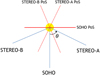 |
Fig. 1. Relative positions of the spacecraft SOHO, STA, and STB and their PoS (red) with the Sun at the center of the graph. θ is the separation angle between the SOHO and STEREO spacecraft. |
The extrapolations were compared with the observations (see Sect. 4) at the source surface, commonly placed at a height of rSS = 2.5 R⊙. At this source-surface radius, the geometry of the extrapolated magnetic field matches the shapes of the coronal structures observed in white-light during solar eclipses best, especially the size of the streamers and coronal hole boundaries (Wang 2009; Wang et al. 2010). Some authors (e.g., Lee et al. 2011) have shown that using smaller source surface heights gives improved agreement between the EUV images and the modeled open field regions during low solar activity periods. They also suggested that the source surface height changes over time and that the energy balance may be different from one solar minimum to the next, depending on both the polar and overall photospheric field strengths and on the open field topology. We nevertheless decided to perform the PFSS extrapolations at 2.5 R⊙ to better compare our work with most of the previous efforts.
In Fig. 2 we show the CR 2091 Carrington maps at 2.5 R⊙ from STB/COR1, SOHO/C2, and STA/COR1 data (from top to bottom) for the east and the west limb of the Sun (left and right column, respectively). In this work we represent images in a reverse color scale, so that brighter coronal features, which correspond to regions of higher electron density, are displayed in darker colors. We combined these maps in a single near-synchronic synoptic map of the corona as described in the following section, thus facilitating a comparison with the results of the photospheric extrapolations described in Sect. 3.
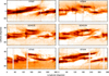 |
Fig. 2. Carrington maps at 2.5 R⊙ for CR 2091 from STB/COR1 (top), SOHO/C2 (middle), and STB/COR1 (bottom) for the east and west limb of the Sun (left and right column, respectively). Images are displayed in a reverse color scale, i.e., brighter coronal features are shown in darker colors. |
2.1. Coronagraphic CR maps
Coronagraphic CR maps result from synoptic maps that are built by extracting from each image a circular profile at a given heliocentric height. These annular slices are then piled up, each column representing one circular profile in the original image. In the synoptic maps, the X-axis gives the time of the observations. The differences with the CR maps lie in the parameterization of the axis: the X-axis gives the Carrington longitude, and the Y-axis the Carrington latitude. Thus, we have a map of the solar corona at a certain radial distance from the solar center.
2.2. Combined CR maps
To combine the six CR maps from the three spacecraft, we first normalized each image to its maximum value; in the case of STA and STB images, it was necessary to subtract a constant value before the normalization process. This background value was estimated at the 10th percentile of the image histogram. Even so, a noticeable asymmetry between the two poles remains in the CR images from both STEREO spacecraft (see, e.g., the top right panel in Fig. 2, where the intensities between the positive and negative latitudes are clearly different). Inspection of some of the original coronal images reveals that the asymmetry likely indicates an asymmetry of the instrumental straylight. Because we are interested in the brightest features of these CR maps, we did not attempt to further correct for this effect.
We then resampled all images to a common longitude and latitude grid. Because each Carrington longitude in a CR map corresponds to a given observing time of the corona, the six CR maps can be displayed on a common time line, as shown in Fig. 3, by means of the temporal distance, Δt, of each longitude slice with respect to a reference time. We chose 20 December 2009 20:00 UT (the center date of CR 2091) as the reference time. With this representation, it is easy to verify that the entire corona is observed by the three instruments over a time range of little more than four days around the reference date of 20 December 2009. In the blue boxes we highlight the coronal sections observed by each instrument.
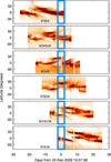 |
Fig. 3. Normalized Carrington maps (same as Fig. 2) at 2.5 R⊙ for CR 2091 from STB, SOHO, and STA, aligned to a common reference time. The blue box indicates the parts of the maps observed within ±2 days from the center date of CR 2091. By collating these six boxes (starting from STB east and ending with STA west), we can obtain a near-synchronic (to within about five days) map of the entire corona. |
We wish to determine a CR map representing the configuration of the corona in as short a time interval as possible (a “near-synchronic” CR map), thus minimizing the effect of the evolution of coronal structures. With the three spacecraft in the favorable configuration shown in Fig. 1, it is indeed possible to scan the entire corona in about 1/6th of a Carrington rotation (with an average angle of 66° between the spacecraft and an average rotation time of 27.3 days, the time needed to span that angle is 27.3 × 66/360 = 5.00 days) is an already significant improvement over the assumption underlying the typical usage of CR maps from a single vantage point, that is, that the corona does not significantly change during a solar rotation.
In this context, it is also useful to note that a polarized brightness (pB) observation at 2.5 R⊙ of an axisymmetric coronal structure at the solar equator is the result of the integration along of the line of sight of a kernel with a full width at half-maximum FWHM ∼ 45°. This angular extent is spanned by the PoS rotating with the Sun in about five days. We can consider this value as an upper limit of the intrinsic ambiguity in longitude of a CR map in the equatorial regions. More realistic values have been determined for instance by Thernisien & Howard (2006), who presented a 3D reconstruction of the electron density of a streamer, and also characterized its length and thickness. For a streamer observed by LASCO on January 2004 during CR 2012, they found that the FWHM of the streamer normalized brightness along the line of sight was ∼8° at 2.5 R⊙, a value corresponding to ∼0.6 days. More importantly, they also found that observed changes in the streamer appearance were due to changes in the viewing geometry, while the intrinsic properties of the streamer did not significantly change over the time interval (about seven days) needed to observe the streamer from edge-on to face-on. With these considerations in mind, and with the obvious exception of events like coronal mass ejections (CMEs), we can reasonably expect that a CR map built over about five days, as is the case of our present study, is as close to a snapshot of the corona around a given date as it could be obtained with this approach.
After the six Carrington maps were scaled to common intensity and coordinate ranges, we used the following two methods to obtain a combined Carrington map representing a near-synchronic map of the solar corona around a chosen reference time, in this case, the middle time of the time interval considered (CR 2091):
-
“Joined map”. At each Carrington longitude, the slice of a normalized CR map whose observing time is closest to the reference time is selected. The advantage of this method is its simplicity; the resulting combined map, however, exhibits noticeable discontinuities at the times where two spacecraft observe the same longitude at similar temporal distance from the reference time.
-
“Merged map”. At each Carrington longitude, the weighted average of all the normalized CR maps for that longitude is computed, where the weight assigned to the ith map is a function of the temporal distance to the reference time of the observation of that slice at that longitude, Δti. In particular, we chose weights proportional to 1/[1+(16 Δti)2], where the time distance is measured in units of the mean synodic period of the Carrington system (27.2753 days). The advantage of this method is that it produces smoother maps that are easier to analyze (data gaps in CR maps are also filled in by other maps). The choice of the kernel width (6.8 days = 1/4 of a CR) is dictated by the considerations of the intrinsic longitudinal uncertainty of the CR maps discussed above and by the mean angular distance between the spacecraft. The FWHM of any kernel, after the weights are normalized, has as a lower limit the difference in time before one spacecraft has the same view as another. Figure 4 illustrates the weighted averaging of this second method for a single longitude (45°). Because the chosen kernel width is longer than about five days, we would need about two more days of observations with respect to those needed to obtain a combined near-synchronic map with the first method, the joined map. Even so, as Fig. 4 shows, the CR map slice that contributes most to the merged-map slice (black line) is the one with only 1.1 days distance from the reference time (slice of STB/E, cyan line), thus inside five days.
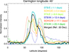 |
Fig. 4. Normalized intensity of the slices at 45° longitude of the six Carrington maps represented in Fig. 2 at 2.5 R⊙ for CR 2091 (color-coding given in the figure legend), together with the weighted averaged intensity computed as described in Sect. 2.2, shown as a solid black line and indicated as “Merged” in the legend. The slices closest in time to the reference time (Δti at 45° longitude, for each map, as indicated in the legend) are also shown using thicker lines. The slice contributing mostly to the merged slice (black line) is the one with Δti at that longitude of 1.1 days (slice of STB/E, cyan line). |
The maps resulting from the application of these two methods are shown in Fig. 5. In our analysis, we did not take into account that the two STEREO spacecraft have a non-zero inclination angle (∼3°) to the ecliptic plane with respect to SOHO. However, these angular differences are too small to affect the brightness of the white-light observations and/or line-of-sight integrations (see discussion above).
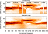 |
Fig. 5. CR 2091 maps, at 2.5 R⊙ obtained by combining the west and east limb Carrington maps for all the three spacecraft with the two methods described in Sect. 2.2. |
To compare these near-synchronic maps with the solutions of the magnetic field extrapolations described in Sect. 3, we need to define which visible structures in the combined maps of Fig. 5 are good proxies for the position of the magnetic neutral line at 2.5 R⊙. As already mentioned in the introduction, it is generally accepted that streamers are the result of the line-of-sight viewing of the heliospheric plasma sheet centered at the magnetic neutral line (Koomen et al. 1998). We therefore compared the position of the streamers in the observed Carrington maps by taking the peaks of absolute and relative maximum values of intensity above a fixed threshold at each date with the extrapolated neutral lines, assuming that the density enhancements corresponding to the intensity peaks track the position of the magnetic neutral line. In Fig. 6 we show the Carrington maps for the east and west limb from the three different coronagraphs on STA, SOHO, and STB, as well as the resulting merged combined map (bottom panel). The cyan lines in the bottom panel mark the intensity peaks. The blue contour defines the part of the maps that is observed at the same time by the instruments and merged in the bottom map. The positions of the main intensity peaks identified in the joined combined map are not significantly different, and thus are not shown here.
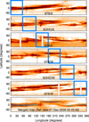 |
Fig. 6. East and west limb Carrington maps observed by the STA/COR1, SOHO/C2, and STB/COR1 coronagraphs for the CR 2091, at 2.5 R⊙ and the merged map obtained by their combinations (bottom panel); the position of the streamer cusps (cyan lines) are overplotted. The blue box defines the part of the maps that is observed at the same time by the instruments. |
2.3. Data analysis
Figure 6 shows that at many longitudes (i.e., between ∼0 − 140°), two observed streamers exist at different latitudes. In addition to the rotational effects (arc-like features as in Fig. 2 at ∼40° latitude and between ∼240 ° −290° longitude), where individual structures appear to move to higher or lower apparent latitudes as they rotate away from or toward the plane of the sky (Liewer et al. 2001), we have to consider that some of the observed features may not correspond to a classic helmet streamer but to a pseudostreamer (Wang et al. 2007). Both helmet streamers and pseudostreamers contribute to the brightness of the K corona, but only the former are associated with interplanetary sector boundaries and the heliospheric current sheet. The way to distinguish between a streamer or a pseudostreamer is through coronal magnetic field extrapolations. Other characteristic features of pseudostreamers that are more difficult to observe, however, are low-lying cusps and two underlying filament channels (Wang et al. 2007). In the case of our data set, we do not see any of these observational signatures that could have helped distinguishing between a streamer or a pseudostreamer without resorting to extrapolations. Because we are unable to determine observationally whether one of the two cyan lines in the bottom panel of Fig. 6 represents a pseudostreamer, we compared both lines with the extrapolated neutral lines.
For the completeness of the discussion, we report that Noci et al. (1997) have previously observed streamers with a bifurcated aspect in the O VI image with the UltraViolet Coronagraph Spectrometer (UVCS, Kohl et al. 1995) on board SOHO, which appeared to consist of two substreamers, or rather three at lower heliocentric distances (∼2 R⊙). They suggested and observed in the Fe XIV line a quadrupolar magnetic configuration at the coronal base with three associated current sheets that gave a signature in the O VI observations but not in Ly-α (except, perhaps, at very low heights).
From now on, we refer to the enhancements observed in the Carrington maps as observed peaks of intensity, generically. Fig. 6 also shows other features such as the CMEs, which appear as vertical and sudden brightenings (see, e.g., at ∼75° or ∼140°).
3. Extrapolations
A variety of magnetic field extrapolation techniques exists, such as PFSS, nonlinear force-free field (NLFFF), magneto-frictional, and full magnetohydrodynamics (MHD) approaches. A detailed description of these techniques can be found in Mackay & Yeates (2012). Here, we perform PFSS extrapolations, starting from different sets of photospheric data (described in detail later in this section), and evaluate their performance by comparing the extrapolations with near-synchronic coronagraphic white-light CR maps of the corona near the source surface. We compare the position of the streamers in the Carrington maps with the neutral lines obtained from four different sets of calculations: methods 1−4. The characteristics of the four models are summarized in Table 1.
Characteristic of the four extrapolation methods used in this work.
The first two methods (methods 1 and 2) use magnetic field extrapolation of synoptic magnetograms and give as result a unique source surface synoptic chart for a Carrington rotation, that is, we have one neutral line for each of these two methods to compare with the observations. The other two methods, methods 3 and 4, instead use synchronic (or time-evolved) photospheric maps of the magnetic field and can produce instantaneous or six-hour maps of the coronal magnetic field. Hence, it is possible to have a coronal map for each instant of the Carrington rotation. We chose to retrieve the magnetic neutral line with methods 3 and 4 on three days during the CR as explained below.
For method 1, we used the magnetic neutral line from the Wilcox Solar Observatory (WSO) online archive1. For the other methods, we derived the neutral line via extrapolations. The four extrapolation methods work as follows.
Method 1 uses a PFSS extrapolation from the WSO synoptic maps and is described in Schatten et al. (1969), Altschuler & Newkirk (1969), and Hoeksema et al. (1983). It assumes that the field in the photosphere is radial and forced to be radial at the source surface (placed at 2.5 R⊙) to approximate the effect of the accelerating solar wind on the field configuration. The result of this extrapolation is a source surface synoptic chart for each Carrington rotation. The range of dates on which the synoptic photospheric map is built is the range of CR 2091 (7 December 2009 – 3 January 2010). In particular, the days of contributing magnetograms are 17−20 and 22−24 December 2009, and 3−4 January 2010. The missing data are interpolated.
Method 2 starts again with the WSO synoptic photospheric maps, but uses a slightly different PFSS extrapolation following the general method and polar-field correction of Wang & Sheeley (1992). This correction enhances the polar field strength, which is meant to better reproduce the open flux in the interplanetary medium, and it also allows the surface field to depart from strict radiality.
Method 3 performs the same PFSS extrapolation as in method 2, but starting from the Michelson Doppler Imager (MDI) observations of the photosphere. To obtain a more realistic estimate of the global photospheric magnetic field distribution, method 3 applies a flux transport model to the photospheric data described in Schrijver & De Rosa (2003). With this extrapolation method, we produced a unique map of the solar corona every six hours, and we chose three days, one at the beginning, one at the middle, and one at the end of the CR 2091 to obtain a neutral line to compare with the observations. The chosen dates are 7 December 2009, 20 December 2009, and 3 January 2010.
Method 4 uses a PFSS extrapolation as in methods 2 and 3 from the Air Force Data Assimilative Photospheric Flux Transport model (ADAPT, Arge et al. 2013). The ADAPT model generates more realistic global solar photospheric magnetic field maps, starting from NSO/GONG data, in our case. ADAPT produces ensemble synchronic predictions (i.e., multiple maps), and in particular, for our work, it produced 12 solutions (depending on different choices of the physical parameters in the simulation, to cover the uncertainty related to those parameters) for each predicted day of the Carrington map. We chose to have extrapolated data for the same three days as for method 3.
4. Results and discussion
We start with the comparison between the streamer intensity peaks and the neutral lines calculated with method 4. As we explained in Sect. 3, this method produces 12 solutions for the coronal magnetic field and accordingly, 12 neutral lines for each day for which an extrapolation was performed. In Fig. 7 we show the neutral lines (black lines) obtained for the 20 December 2009 extrapolation. We plot the peaks of streamer intensity (cyan lines) on the merged Carrington map from the bottom panel of Fig. 6. The differences among the 12 extrapolated neutral lines are no more than 20°. Although we show the results for only one of the three days of extrapolations, the same finding holds for the other two days. We therefore show only one of these extrapolations from now on. To measure the difference between streamers and calculated HCS, we used the absolute value of the latitudinal difference, |Latobs − Latext|, between the two features at each longitude. Because there are two streamers belts between ∼0 and 140°, we performed the calculation of these differences for two cases, one considering the points with the highest latitudes (Latobs1, case 1), and the other considering the points with the lowest latitudes (Latobs2, case 2). For method 4, we then plot the extrapolated neutral line that has the best fit with one of the two lines representing the observations, calculated as the mean value of |Latobs − Latext|.
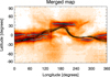 |
Fig. 7. Merged Carrington map with the streamer axes (cyan lines) and calculated neutral lines (black lines) from method 4 for 20 December 2009. |
In Fig. 8 we compare the streamer axes with the neutral lines derived from all four extrapolation methods on the merged Carrington map. For methods 1 and 2, we plot one neutral line (solid green and magenta lines, respectively), while for methods 3 and 4, we plot three neutral lines corresponding to the three days chosen to perform the extrapolations (three dashed lines for method 3 and three dash-dotted lines for method 4, plotted with different colors to distinguish among the days: black for 7 December 2009, white for 20 December 2009, and blue for 3 January 2010).
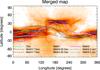 |
Fig. 8. Merged Carrington map. The observed intensity peaks (cyan lines) and the neutral lines obtained from the four methods of extrapolation described in Sect. 3 are overplotted. The color-coding is given in the figure legend. |
Even though the extrapolations use the same photospheric magnetic field data (WSO synoptic maps) and the PFSS methods are very similar, methods 1 and 2 provide different results. The main difference lies between 0 and 100° longitudes, where we also have two streamer axes, one at ∼0° latitude and the other at ∼ − 20°: the neutral line from method 1 overlaps the observation at ∼0° latitude, while the neutral line from method 2 overlaps the one at ∼ − 20° latitude.
Regarding methods 3 and 4, we note that the neutral lines obtained from the extrapolations computed on three different days can be very different because the magnetic field in the photosphere can change during one solar rotation. A strong bipolar region indeed emerges between (60 ° , − 60 ° ) Carrington coordinates at the end of the Carrington rotation.
To evaluate the longitudinal dependence of the accuracy of the extrapolations, we plot in Fig. 9 the quantity Latobs − Latext as a function of the longitude for the two streamer axes, Latobs1 (top panels) and Latobs2 (bottom panels). Table 2 summarizes the means of the absolute value of the differences, and the standard deviations of these differences. We note that the two metrics are very well correlated.
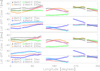 |
Fig. 9. Latitudinal differences between the extrapolated neutral lines and the two streamer axes as a function of the longitude. The color-coding is given in the figure legend. |
Means of the absolute value of the differences between the extrapolated neutral line latitudes and that of the observed streamers and the standard deviation of these differences for the two streamer axes.
We see that four neutral lines (method 1 for case 1, method 2 for case 2, and method 4 (20 December) for both cases 1 and 2) give a good approximation of the streamers position with a mean error of ∼9 − 12° and a standard deviation of ∼11 − 12° with respect to the other methods. Of these four, method 1 is the method that gives the neutral line with the absolute best agreement with the observations, assuming that the streamer between 0 and 120° longitude has a latitude of ∼0°. When we compare the values of the means and the standard deviations in Table 2 for cases 1 and 2 for all the methods, there is no evidence of a better agreement of the extrapolated neutral lines with one or the other streamer we observe between 0 and 120° longitude. Thus, neither the observations nor the extrapolations allow us to discern the presence of a pseudostreamer in this CR.
We find a good agreement with the neutral lines extrapolated from methods 1 and 2 (based on synoptic maps) but also from method 4 (based on the synchronic map for 20 December 2009). When we consider the photospheric synoptic maps used in the first two methods in detail, we see that the days of magnetogram observations contributing to the synoptic map are 17−20 and 22−24 December 2009 and 3−4 January 2010, with the missing data interpolated. This means that we have a synoptic map of the photospheric magnetic field that was built mainly using data that were acquired around 20 December, which is the date we chose as the reference time to build the near-synchronic coronal map. The main uncertainties in the comparison of the neutral lines from methods 1 and 2 and the observed streamers are at small longitudes (30 − 90°, which correspond to the dates of 3−4 January 2010), where the photospheric magnetic field changes due to the emergence of a strong bipolar region.
5. Conclusions
The aim of this study was to find a fast and reliable method to systematically validate the various methods of coronal magnetic field extrapolations. For this purpose, we determined the position of the coronal streamers by their intensity peaks and compared them with the location of the magnetic neutral lines obtained from four different coronal magnetic field extrapolation methods. The comparison was based on the assumption that the intensity enhancements track the position of the streamers and the associated magnetic neutral line at 2.5 R⊙. This assumption is not always true because a denser sheet of plasma that is visible as a bright enhancement in the white-light observations can also be related to a pseudostreamer that does not enclose a current sheet. Observationally, at least for CR 2091, we cannot distinguish between streamers and pseudostreamers, but we can still derive useful information about the reliability of the extrapolations.
The improvement of our study with respect to the previous attempts of comparing the position of the streamers in white-light Carrington maps and extrapolated neutral lines (see Sect. 1) is in the combination of SOHO/LASCO-C2, STA, and STB/SECCHI-COR1 Carrington maps at 2.5 R⊙ for Carrington rotation CR 2091 to obtain a synoptic map of the solar corona with the minimum amount of temporal evolution and then compare the coronal structures visible in this coronagraphic map with magnetic field extrapolations.
The four extrapolation methods are described in Sect. 3. The first two methods are based on synoptic photospheric maps and provide one neutral line to be compared with the observations. Methods 3 and 4 instead produce instantaneous coronal magnetic field maps starting from synchronic photospheric maps for each instant of the CR. For these two methods, we chose the extrapolated magnetic neutral line for three days during the CR. Moreover, method 4 produced 12 neutral lines for each day. We find that the differences among these neutral lines are too small to let us distinguish among them through a comparison with the observations. We do not need such a high resolution in the extrapolations for this type of analysis.
Considering the results of methods 3 and 4, we find that the neutral lines obtained from three different days during the Carrington rotation can be very different because the photospheric field data may change on a timescale shorter than 13 days (minimum temporal distance between the dates chosen). This result underlines the importance of reducing the time needed to scan the corona, for example, by combining images from instruments that scan the Sun from different viewing angles. After Solar Orbiter is launched, there will be several coronagraphs in space: Metis (Antonucci et al. 2012) on Solar Orbiter itself, and ASPIICS on PROBA-3 (Lamy et al. 2010; Renotte et al. 2016) to coordinate for joint observation campaigns. We have to take into account that for some instruments such as Metis, which will also observe out of the ecliptic plane, other techniques may be required, such as tomography, to compare the data with the other coronagraphs. Tomography is of course a valid approach also from inside the ecliptic, but its use is beyond the scope of this work. Solar Orbiter will also host a magnetograph, the Polarimetric and Helioseismic Imager (PHI, Gandorfer et al. 2011; Solanki et al. 2015), which will provide magnetograms of the solar photosphere. In this way, we will also have simultaneous maps of the photospheric magnetic field available over more than just the solar surface that is visible from Earth.
Comparing the neutral lines resulting from the four methods and the positions of the streamers, we find a good agreement for methods 1, 2, and 4 (performed on 20 December 2009). We note that all three methods start from photospheric maps of the magnetic field (synoptic or synchronic) built with data acquired around the same day we have chosen as the reference time to build the merged coronal map from the contributions of the Carrington maps of the three spacecraft. This is not a necessary condition, however, to have a good extrapolation, because the magnetic neutral line extrapolated using method 3 (on 20 December 2009) gives a larger error than the observations (see Table 2), at least for CR 2091. A detailed comparison of the different extrapolation methods will be the subject of a subsequent paper.
The method described in this paper has clear advantages in its simplicity and in the availability of the observations and extrapolations, but it can fail in some situations, for instance, when there are many white-light features at different latitudes that make an interpretation ambiguous. We achieved a decent overall agreement at the Carrington longitudes for which the position of the streamers is unique and a significant disagreement at Carrington longitudes where many white-light features arise. The current set of extrapolations is not useful beyond a top-level comparison with the coronagraphic images (i.e., the existence of a streamer at a given position angle). They seem to lack reliable information on the field to go beyond this. This study furthermore shows that different magnetogram sources may also disagree.
We plan to repeat the multi-viewpoint analysis presented in this paper with other CR maps to cover at least one solar cycle. It would also be interesting to compare the combined quasi-synchronic maps with results from other extrapolations than those we used for this work. We also plan to identify other visible structures in the white-light maps (e.g., the position of the coronal holes) to compare them with the extrapolation results.
Acknowledgments
The Wilcox Solar Observatory data used in this study were obtained via the web site http://wso.stanford.edu at 2016:12:09_03:10:30 PST courtesy of J.T. Hoeksema. The Wilcox Solar Observatory is currently supported by NASA. The SOHO/LASCO data used here are produced by a consortium of the Naval Research Laboratory (USA), Max-Planck-Institut for Sonnensystemforschung (Germany), Laboratoire d’Astrophysique Marseille (France), and the University of Birmingham (UK). SOHO is a project of international cooperation between ESA and NASA. C.S., V.A., A.B., S.D., D.S., R.S., E.A., V.D.D., S.F., F.F., F.L., G.Na., G.Ni., P.N., M.P., M.R., D.T. and R.V. acknowledge the support of the Italian Space Agency (ASI) to this work through contract ASI/INAF No. I/013/12/0. A.V. is supported by NRL N00173-16-1-G029 and NASA NNX16AH70G grants.
References
- Altschuler, M. D., & Newkirk, Jr., G. 1969, Sol. Phys., 9, 131 [Google Scholar]
- Antonucci, E., Fineschi, S., Naletto, G., et al. 2012, SPIE, 8443, 9 [Google Scholar]
- Arge, C. N., Henney, C. J., Hernandez, I. G., et al. 2013, AIP Conf. Proc., 1539, 11 [NASA ADS] [CrossRef] [Google Scholar]
- Brueckner, G. E., Howard, R. A., Koomen, M. J., et al. 1995, Sol. Phys., 162, 357 [NASA ADS] [CrossRef] [Google Scholar]
- Bruno, R., Burlaga, L. F., & Hundhausen, A. J. 1982, J. Geophys. Res., 87, 10339 [NASA ADS] [CrossRef] [Google Scholar]
- Domingo, V., Fleck, B., & Poland, A. I. 1995, Sol. Phys., 162, 1 [NASA ADS] [CrossRef] [Google Scholar]
- Gandorfer, A., Solanki, S. K., Woch, J., et al. 2011, J. Phys. Conf. Ser., 271, 012086 [NASA ADS] [CrossRef] [Google Scholar]
- Hoeksema, J. T., Wilcox, J. M., & Scherrer, P. H. 1983, J. Geophys. Res., 88, 9910 [NASA ADS] [CrossRef] [Google Scholar]
- Howard, R. A., & Koomen, M. J. 1974, Sol. Phys., 37, 469 [NASA ADS] [CrossRef] [Google Scholar]
- Howard, R. A., Moses, J. D., Vourlidas, A., et al. 2008, Space Sci. Rev., 136, 67 [NASA ADS] [CrossRef] [Google Scholar]
- Kaiser, M. L., Kucera, T. A., Davila, J. M., et al. 2008, Space Sci. Rev., 136, 5 [NASA ADS] [CrossRef] [Google Scholar]
- Kohl, J. L., Esser, R., Gardner, L. D., et al. 1995, Sol. Phys., 162, 313 [NASA ADS] [CrossRef] [Google Scholar]
- Koomen, M. J., Howard, R. A., & Michels, D. J. 1998, Sol. Phys., 180, 247 [NASA ADS] [CrossRef] [Google Scholar]
- Lamy, P., Damé, L., Vivès, S., & Zhukov, A. 2010, SPIE, 7731, 18 [Google Scholar]
- Lee, C. O., Luhmann, J. G., Hoeksema, J. T., et al. 2011, Sol. Phys., 269, 367 [Google Scholar]
- Liewer, P. C., Hall, J. R., De Jong, M., et al. 2001, J. Geophys. Res., 106, 15903 [NASA ADS] [CrossRef] [Google Scholar]
- Mackay, D. H., & Yeates, A. R. 2012, Sol. Phys., 9, 6 [Google Scholar]
- Müller, D., Marsden, R. G., & St. Cyr, O. C. & Gilbert, H. R., 2013, Sol. Phys., 285, 25 [NASA ADS] [CrossRef] [Google Scholar]
- Noci, G., Kohl, J. L., Antonucci, E., et al. 1997, Adv. Space Res., 20, 2219 [NASA ADS] [CrossRef] [Google Scholar]
- Rachmeler, L. A., Platten, S. J., Bethge, C., Seaton, D. B., & Yeates, D. B. 2014, ApJ, 787, L3 [NASA ADS] [CrossRef] [EDP Sciences] [Google Scholar]
- Renotte, E., Buckley, S., Cernica, I., et al. 2016, SPIE, 9904, 3D [Google Scholar]
- Saez, F., Zhukov, A. N., Lamy, P., & Llebaria, A. 2005, A&A, 442, 351 [Google Scholar]
- Schatten, K. H., Wilcox, J. M., & Ness, N. F. 1969, Sol. Phys., 6, 442 [Google Scholar]
- Schrijver, C. J., & De Rosa, M. L. 2003, Sol. Phys., 212, 165 [Google Scholar]
- Solanki, S. K., del Toro Iniesta, J. C., Woch, J., et al. 2015, in Polarimetry, eds. K. N. Nagendra, S. Bagnulo, R. Centeno, & M. Jesús Martínez González, IAU Symp., 305, 108 [NASA ADS] [Google Scholar]
- Thernisien, A. F., & Howard, R. A. 2006, ApJ, 642, 523 [NASA ADS] [CrossRef] [Google Scholar]
- Wang, Y.-M. 2009, Space Sci. Rev., 144, 383 [NASA ADS] [CrossRef] [Google Scholar]
- Wang, Y.-M., & Sheeley, N. R. 1992, ApJ, 392, 310 [NASA ADS] [CrossRef] [Google Scholar]
- Wang, Y.-M., Sheeley, N. R., Howard, R. A., et al. 1997, ApJ, 485, 875 [Google Scholar]
- Wang, Y.-M., Sheeley, N. R., & Rich, N. B. 2000, Geophys. Res. Lett., 27, 149 [NASA ADS] [CrossRef] [Google Scholar]
- Wang, Y.-M., Sheeley, N. R., & Rich, N. B. 2007, ApJ, 658, 1340 [NASA ADS] [CrossRef] [Google Scholar]
- Wang, Y.-M., Robbrecht, E., Rouillard, A. P., Sheeley, N. R., & Thernisien, A. F. R. 2010, ApJ, 715, 39 [NASA ADS] [CrossRef] [Google Scholar]
- Wilcox, J. M., & Hundhausen, A. J. 1983, J. Geophys. Res., 88, 8095 [NASA ADS] [CrossRef] [Google Scholar]
- Zhao, X. P., Hoeksema, J. T., & Rich, N. B. 2002, Adv. Space Res., 29, 441 [NASA ADS] [CrossRef] [Google Scholar]
All Tables
Means of the absolute value of the differences between the extrapolated neutral line latitudes and that of the observed streamers and the standard deviation of these differences for the two streamer axes.
All Figures
|
Fig. 1. Relative positions of the spacecraft SOHO, STA, and STB and their PoS (red) with the Sun at the center of the graph. θ is the separation angle between the SOHO and STEREO spacecraft. |
| In the text | |
|
Fig. 2. Carrington maps at 2.5 R⊙ for CR 2091 from STB/COR1 (top), SOHO/C2 (middle), and STB/COR1 (bottom) for the east and west limb of the Sun (left and right column, respectively). Images are displayed in a reverse color scale, i.e., brighter coronal features are shown in darker colors. |
| In the text | |
|
Fig. 3. Normalized Carrington maps (same as Fig. 2) at 2.5 R⊙ for CR 2091 from STB, SOHO, and STA, aligned to a common reference time. The blue box indicates the parts of the maps observed within ±2 days from the center date of CR 2091. By collating these six boxes (starting from STB east and ending with STA west), we can obtain a near-synchronic (to within about five days) map of the entire corona. |
| In the text | |
|
Fig. 4. Normalized intensity of the slices at 45° longitude of the six Carrington maps represented in Fig. 2 at 2.5 R⊙ for CR 2091 (color-coding given in the figure legend), together with the weighted averaged intensity computed as described in Sect. 2.2, shown as a solid black line and indicated as “Merged” in the legend. The slices closest in time to the reference time (Δti at 45° longitude, for each map, as indicated in the legend) are also shown using thicker lines. The slice contributing mostly to the merged slice (black line) is the one with Δti at that longitude of 1.1 days (slice of STB/E, cyan line). |
| In the text | |
|
Fig. 5. CR 2091 maps, at 2.5 R⊙ obtained by combining the west and east limb Carrington maps for all the three spacecraft with the two methods described in Sect. 2.2. |
| In the text | |
|
Fig. 6. East and west limb Carrington maps observed by the STA/COR1, SOHO/C2, and STB/COR1 coronagraphs for the CR 2091, at 2.5 R⊙ and the merged map obtained by their combinations (bottom panel); the position of the streamer cusps (cyan lines) are overplotted. The blue box defines the part of the maps that is observed at the same time by the instruments. |
| In the text | |
|
Fig. 7. Merged Carrington map with the streamer axes (cyan lines) and calculated neutral lines (black lines) from method 4 for 20 December 2009. |
| In the text | |
|
Fig. 8. Merged Carrington map. The observed intensity peaks (cyan lines) and the neutral lines obtained from the four methods of extrapolation described in Sect. 3 are overplotted. The color-coding is given in the figure legend. |
| In the text | |
|
Fig. 9. Latitudinal differences between the extrapolated neutral lines and the two streamer axes as a function of the longitude. The color-coding is given in the figure legend. |
| In the text | |
Current usage metrics show cumulative count of Article Views (full-text article views including HTML views, PDF and ePub downloads, according to the available data) and Abstracts Views on Vision4Press platform.
Data correspond to usage on the plateform after 2015. The current usage metrics is available 48-96 hours after online publication and is updated daily on week days.
Initial download of the metrics may take a while.