| Issue |
A&A
Volume 626, June 2019
|
|
|---|---|---|
| Article Number | A26 | |
| Number of page(s) | 12 | |
| Section | Planets and planetary systems | |
| DOI | https://doi.org/10.1051/0004-6361/201935077 | |
| Published online | 06 June 2019 | |
Photometry, spectroscopy, and polarimetry of distant comet C/2014 A4 (SONEAR)
1
Astronomical Institute of the Slovak Academy of Sciences,
05960
Tatranská Lomnica,
Slovak Republic
e-mail: This email address is being protected from spambots. You need JavaScript enabled to view it.
2
Main Astronomical Observatory of the National Academy of Sciences,
27 Akademika Zabolotnoho St.,
03143
Kyiv,
Ukraine
3
Astronomical Observatory, Taras Shevchenko National University of Kyiv,
3 Observatorna St.,
04053
Kyiv,
Ukraine
4
University of Maryland,
College Park,
Maryland,
USA
5
Department of Physics, Assam University,
Silchar
788011,
Assam,
India
6
Special Astrophysical Observatory, Russian Academy of Sciences,
Nizhnii Arkhyz,
Karachay-Cherkessia
369167,
Russia
7
Crimean Astrophysical Observatory,
Nauchnij,
Crimea
8
Ural Federal University,
620083
Ekaterinburg,
Russia
Received:
17
January
2019
Accepted:
4
April
2019
Abstract
Context. The study of distant comets, which are active at large heliocentric distances, is important for a better understanding of their physical properties and mechanisms of long-lasting activity.
Aims. We analyzed the dust environment of the distant comet C/2014 A4 (SONEAR), with a perihelion distance near 4.1 au, using comprehensive observations obtained by different methods.
Methods. We present an analysis of spectroscopy, photometry, and polarimetry of comet C/2014 A4 (SONEAR), which were performed on November 5–7, 2015, when its heliocentric distance was 4.2 au and phase angle was 4.7°. Long-slit spectra and photometric and linear polarimetric images were obtained using the focal reducer SCORPIO-2 attached to the prime focus of the 6 m telescope BTA (SAO RAS, Russia). We simulated the behavior of color and polarization in the coma presenting the cometary dust as a set of polydisperse polyshapes rough spheroids.
Results. No emission features were detected in the 3800–7200 Å wavelength range. The continuum showed a reddening effect with the normalized gradient of reflectivity 21.6 ± 0.2% per 1000 Å within the 4650–6200 Å wavelength region. The fan-like structure in the sunward hemisphere was detected. The radial profiles of surface brightness differ for r-sdss and g-sdss filters, indicating a predominance of submicron and micron-sized particles in the cometary coma. The dust color (g–r) varies from 0.75 ± 0.05m to 0.45 ± 0.06m along the tail. For an aperture radius near 20 000 km, the dust productions in various filters were estimated as Afρ = 680 ± 18 cm (r-sdss) and 887 ± 16 cm (g-sdss). The polarization map shows spatial variations in polarization over the coma from about −3% near the nucleus to −8% at a cometocentric distance of about 150 000 km. Our simulations show that the dust particles are dominated (or covered) by ice and tholin-like organics. Spatial changes in the color and polarization can be explained by particle fragmentation.
Key words: comets: general / comets: individual: C/2014 A4 (SONEAR) / polarization / scattering / methods: miscellaneous
© ESO 2019
1 Introduction
Small ice-rich bodies from the outer regions of the solar system are recognized as remnants of the long-time evolution of protoplanetary nebula. Currently, three main reservoirs of the comets are identified: the trans-Neptunian region, the Oort Cloud, and the Asteroid belt (i.e. main-belt comets and active asteroids) (Dones et al. 2015). Dynamical studies have revealed that (i) the Oort Cloud is a primary source of “nearly isotropic comets,” including long-period (LP) comets and Halley-type comets; (ii) the flattened Kuiper Belt is the source of ecliptic comets and Encke-type comets; and (iii) the Scattered disk is the source of the Jupiter-family comets (JFCs) and Centaurs (Weissman 1990, 1997; Levison et al. 2010). From the dynamical evolutionary scenarios, however, it is not clearly understood if short- and long-period comets formed at distinct places or in the slightly overlapped regions of the primordial planetesimal disk before they were scattered to the outer region of the solar system (Dones et al. 2004, 2015; Levison et al. 2008; Nesvorný et al. 2017).
Remote investigations of primitive matter in the solar system have traditionally been carried out through observations of long-period comets, which are less affected by solar radiation than their short-period counterparts orbiting much closer to the Sun. A dynamically new comet is usually defined as a comet with a semimajor axis of orbit a > 10 000 au, or orbital period P > 1 million yr (Eicher & Levy 2013; Mazzotta Epifani et al. 2014). They reside very far from the Sun and spend the majority of their lifetimes outside the heliosphere. Therefore, these comets are exposed to marginal solar radiation and are modified very little by the solar wind. In spite of this, dynamically new comets are characterized by a higher level of activity on average (Meech et al. 2009; Ivanova et al. 2015b; Sárneczky et al. 2016).
Currently for distant comets, molecular bands in spectra above the underlying continuum have been detected in two comets, 29P/Schwassmann-Wachmann 1 at a heliocentric distance of about 5.9 au, and C/2002 VQ94 (LINEAR) at 7.3 au (Korsun et al. 2006, 2008, and references therein). Tails have not been observed in these comets, and their morphologies are characterized by asymmetric comae with jet features (Stansberry et al. 2004; Korsun et al. 2006, 2008; Trigo-Rodríguez et al. 2008; Ivanova et al. 2016; Picazzio et al. 2019). In other distant comets, gas emission features have not been detected above the reflected solar continuum in the optical spectra, although some of these comets demonstrated long dust tails (Roemer 1962; Belton 1965; Korsun & Chörny 2003; Meech et al. 2009; Ivanova et al. 2015a,b).
The compositional taxonomy of the small icy bodies allows us to establish a possible correlation between physical properties of the distant dwellers and their orbital characteristics, shedding light on the primordial physical conditions at the places of their formation (Mandt et al. 2015). Studies of comets in their active phase can be especially informative. It is especially interesting to trace the activity evolution of the dynamically new comets moving into the inner solar system for the first time and compare it with the activity of returning comets that have had passages through the inner solar system and as a result have their outermost layers differentiated and depleted of volatiles.
The main mechanisms that have been proposed to explain the activity of comets at large heliocentric distances are the phase transition between amorphous and crystalline water ice (Prialnik 1992; Capria et al. 2002), the annealing of amorphous water ice (Meech et al. 2009), and the sublimation of more volatile components like CO and/or CO2. For comets, which are active at heliocentric distances of more than 4 au and where the temperature of the nucleus surface is lower than the H2 O sublimation temperature, the activity is likely supported by the sublimation of more volatile CO2 that was tentatively confirmed by the AKARI observations (Ootsubo et al. 2012) or CO (Jewitt et al. 2019). However, as shown by Ivanova et al. (2011), the upper layers of the cometary nucleus must be peeled off continually in order to satisfy the observational results for a long-term high activity of the comets, and the most popular idea of crystallization of amorphous water ice cannot be responsible for the observed long-term cometary activity at large heliocentric distances.
The volatile molecule abundances do not show any correlation with dynamical families, leading to the conclusion that the two groups of comets were formed in largely overlapping regions (A’Hearn et al. 2012). Contrary to the color diversity in the Kuiper Belt population, no difference was found between the mean colors of the short- and long-period comets, which confirms the absence of significant composition differences between these two groups (Jewitt 2015). Although no difference was found between the mean colors of dynamically new and returning long-period comets (Solontoi et al. 2012), it is very important to continue studying comets from different dynamic groups.
In this work, we investigate one of the new LP comets, C/2014 A4 (SONEAR) (hereafter C/2014 A4). In a circular of the IAU’s Central Bureau for Astronomical Telegrams (CBET #3783), issued on January 16, 2014, a discovery was announced of an apparently asteroidal object (~18.1m) by Cristovao Jacques, Eduardo Pimentel, and Joao Ribeiro de Barros on CCD images obtained on January, 2014, 12.0 UT, with a 0.30 m f/3 reflector of the Southern Observatory for Near Earth Research (SONEAR) at Oliveira, Brazil. The object showed a cometary appearance at perihelion distance 4.18 au (Williams 2014).
We present an analysis of the optical observations of comet C/2014 A4 at a post-perihelion heliocentric distance 4.2 au. The paper is organized as follows. Observations and data reduction are presented in Sect. 2. In Sect. 3 we analyze all the data, including polarimetry. In Sect. 4 we present the modeling of polarization and color. In Sect. 5 we summarize our conclusions.
2 Observations and data reduction
The observations of C/2014 A4 were made with the 6 m telescope known as BTA at the Special Astrophysical Observatoryof the Russian Academy of Sciences (SAO RAS) on November 5, 2015, when the heliocentric and geocentric distance of the comet was 4.2 and 3.3 au, respectively, and the phase angle was 4.7°. The focal reducer SCORPIO-2 attached to the prime focus of the telescope was operated in the photometric, polarimetric, and long-slit spectroscopic modes (Afanasiev & Moiseev 2011). A CCD chip E2V42-90 consisting of 4600 × 2048 px was used as a detector. The size of one pixel is 13.5 × 13.5 μm, which corresponds to 0.18′′ × 0.18′′ on the sky plane.
The photometric data of C/2014 A4 were obtained through the g-sdss (the central wavelength λ0 and FWHM are represented as λ4650/650 Å) and r-sdss (λ6200/600 Å) broadband filters. The seeing was stable around 1.4′′. Performing photometric and polarimetric measurements, we applied a 2 × 2 binning of the original frames. The dimension of the images was 1024 × 1024 px and the scale was 0.36′′ px−1. The full fieldof view of the CCD is 6.1′ × 6.1′. Bias subtraction, flat field correction, and cleaning from cosmic ray tracks were made. The sky background for each individual frame was estimated from those parts of the frame that were not covered by the cometary coma and were free of faint stars, using a procedure of building histogram of counts in the image. Because measurements were differential, we combined the frames of the comet using only the central contour of isophotes closest to the maximum of the comet brightness.
Spectroscopic observations were made with a long-slit mask. The height of the slit was 6.1′ and the width was 1′′. The transparent grism VPHG1200@5401 was used asa disperser in the spectroscopic mode. The spectra covered the wavelength range of 3800–7200 Å and had a dispersion of 0.81 Å px−1. The spectral resolution of the spectra was defined by the width of the slit and was about 5.2 Å. The spectroscopic images were binned along the spatial direction as 1 × 2. We subtracted the bias, performed the flat-fielding, and removed the hits of cosmic rays. The wavelength calibration was performed using the spectrum of a He–Ne–Ar lamp. After that we performed the linearization and summation of the spectra obtained with the same slit position. To estimate a night sky spectrum, we used the peripheral regions of the slit where the comet light contribution was negligible. Then we transformed the peripheral night sky spectrum into the Fourier space and extrapolated it onto the comet position by using the polynomial representation at a given wavelength. The telescope was tracked on the comet to compensate for its apparent motion during the exposure. To provide the absolute photometric and spectral calibration, we observed standard star G191-B2B (Oke 1990) and used the measurements of the spectral atmospherictransparency at the Special Astronomical Observatory provided by Kartasheva & Chunakova (1978). A standard reduction of the obtained spectroscopic data was done. To remove biases from the observed frames, to clean the frames from the cosmic events, and to correct their geometry we used specialized software packages in the IDL environment developed at the SAO RAS. The polarimetric data were obtained with the broadband R (λ6420/790 Å) filter of the Johnson-Cousins photometric system. For measurements of the degree of linear polarization of the comet, we used the dichroic polarization analyzer (POLAROID; Afanasiev & Amirkhanyan 2012). The reduction of the obtained polarimetric images was performed using standard techniques of bias frame subtraction, flat-field correction, and preparation of images for processing. The corrected frames were stacked. We also observed the polarized and non-polarized standard stars from the lists of Hsu & Breger (1982), Schmidt et al. (1992), and Heiles (2000) to determine the instrumental polarization. Typically, the instrumental polarization was less than 0.1%. A detailed description of the data reduction and the method of the calculation of polarization parameters with SCORPIO-2 can be found in Afanasiev & Amirkhanyan (2012), Afanasiev et al. (2014), Ivanova et al. (2009, 2017a), and Rosenbush et al. (2017). The errors in the averaged polarization degree varied from 0.12% in the near-nucleus region to 1.1% in the tail at a projected distance ρ from the coma photocenter ~150 000 km.
The photometric observations of comet C/2014 A4 were also carried out at the 0.4 m MASTER-II-Ural telescope (Kourovka observatory of the Ural Federal University, Russia) on November 7, 2015. The comet was observed through Johnson’s broadband V (λ5510/880 Å) and R (λ6580/1380 Å) filters. The CCD Apogee ALTA U16M CCD was used as the detector with an image size of 4096 × 4096 px and a scale of 1.85′′ px−1.
The viewing geometry and log of observations of comet C/2014 A4 are presented in Table 1, which lists the mid-cycle time; the heliocentric (r) and geocentric (Δ) distances; the phase angle of the comet (α); the position angle of the extended Sun-comet radius vector (ϕ); the filter/grism; the total exposure time during the night (Texp); the number of cycles of observations obtained during night (N); the mode of the observation: Images (Ima), Images of Linear Polarization (ImaLP), or Spectra (SP); and the telescopes.
Log of the observations of comet C/2014 A4 (SONEAR).
3 Photometry: analysis of the observed data
3.1 Morphology
For the morphology analysis, we used the images of comet C/2014 A4 obtained through the broadband g-sdss (λ4650/650 Å) and r-sdss (λ6200/600 Å) filters at the SAO RAS 6 m telescope. Figure 1 shows direct images of comet C/2014 A4 with relative isophots (a) and images treated with digital filters (b–e). To highlight low-contrast structures in the images, we applied a combination of numerical techniques (see Fig. 1): a rotational gradient method (Larson & Sekanina 1984), Gauss blurring, division by azimuthal average, 1/ρ profile method, and median filtering (Samarasinha & Larson 2014). To exclude spurious features when interpreting the obtained images, each of the digital filters was applied with the same processing parameters for all individual exposures. This technique has been used before to pick out structures in several comets with good results (Ivanova et al. 2009, 2016, 2017a, 2018; Rosenbush et al. 2017; Picazzio et al. 2019).
The comet displayed an extended coma with highly condensed material in the near-nucleus area and a long tail in the antisolar direction, typical of most comets active at large heliocentric distances (Korsun & Chörny 2003; Korsun et al. 2008; Ivanova et al. 2015a,b; Sárneczky et al. 2016). We can see in Fig. 1 that there are no features in the tail, butthere is a fan-like structure in the sunward hemisphere, which is labelled J.
3.2 Radial surface brightness profiles
For the analysis of the radial surface brightness profile of the coma and tail, we used the g-sdss and r-sdss images of comet C/2014 A4. The individual curves in Fig. 2 show variations of the average coma flux in the 3 × 3 px size aperture with increasing distance from the nucleus. The cuts across the intensity map of the comet are made in different directions: along (solid line) and perpendicular to (dashed line) the solar direction, and along the tail (dotted line), the position angle of which, measured counterclockwise from north through east, is 121°. Figure 2 shows large differences between the profiles of the tail and coma and between sunward and perpendicular to solar. There is a gentle decline in the surface brightness in the tail, while a sharp drop in brightness is seen in the coma. The values of the slopes for radial profiles of surface brightness of the coma and tail of comet C/2014 A4 are presented inTable 2. In the case of a steady-state and free expansion of long-lived grains, the n value in the dependence I ∝ ρn, which describes the brightness variations with cometocentric distance ρ, should be −1. The table shows that the intensity decrease with distance from the nucleus is not uniform. The slopes change with cometocentric distance, and this change is different for the g-sdss and r-sdss filters. Sincethe slopes differ significantly for the coma and tail, and they also change with increasing distance from the nucleus, we can assume that there is a non-isotropic dust emission from the nucleus, which forms some structures in the innermost coma and tail.
3.3 Color and dust productivity
Using photometric observations, we determined the magnitude, dust color, and dust productivity (in the sense of Afρ) for both observation dates. The cometary magnitude can be computed from the expression
![Mathematical equation: \begin{equation*} m_{\textrm{c}} = -2.5 \log_{10} \left[ \frac{I_{\textrm{c}}(\lambda)}{I_{\textrm{s}}(\lambda)} \right] + m_{\textrm{s}} - 2.5 \log_{10} p(\lambda){\Delta} M ,\, \end{equation*}](/articles/aa/full_html/2019/06/aa35077-19/aa35077-19-eq1.png) (1)
(1)
where mc is the comet integrated magnitude calculated for the aperture of radius ρ; Ic and Is are the measured fluxes of the comet and the standard star in counts, respectively; ms is the star magnitude; p(λ) is the sky transparency, which depends on the wavelength; and ΔM is the difference between the airmasses of the comet and the star.
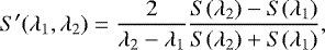
To create a color map of the dust coma and tail (Fig. 3, left), we converted each pixel for summed images g-sdss and r-sdss into the apparent magnitude and created the final (g–r) color map by subtracting the two sets of images from each other. An average error in the magnitude measurements is 0.04m. By analyzing the color map (Fig. 3), we can see that the dust color (g–r) of comet C/2014 A4 is mainly red, especially in the tail direction. The (g–r) color varies from 0.75 ± 0.05m in the near-nucleus area to 0.45 ± 0.06m along the tail; instead, in the anti-tail direction, the comet showed another color distribution. In this region, the color of the dust is mostly neutral (~0.45m) in comparison with the Sun’s color ((g–r) for the Sun2 is 0.44m). Digital processing of the images showed a fan-like structure (see Fig. 1) in this area.
We also estimated the parameter Afρ, which was introduced by A’Hearn et al. (1984). This parameter characterizes the dust production rate of a comet and is determined by the ratio of the effective scattering cross section for all the grains entering the field of view of the detector to the projection of this field of view onto the celestial sphere. To calculate values of Afρ, we used comet magnitudes obtained with different aperture radii. For the aperture radius ~20 000 km, the comet magnitude 15.45 ± 0.05m was derived for g-sdss filter and 16.12 ± 0.03m for r-sdss filter. Using observations performed with the 6 m telescope in the r-sdss band, we calculated Afρ = (680 ± 18) cm for an aperture size of 20 000 km. The dust productions in broadband V and R filters (MASTER-II telescope) were estimated as Afρ = 659 ± 39 cm and 645 ± 36 cm, respectively, for the same aperture radius, which are close to the results obtained via the 6 m telescope.
This value of dust productivity is similar to the value estimated for comet C/2014 A43. Also, our results are close to the data obtained by Mauro Facchini (Cavezzo Observatory and Celado Observatory) and Rolando Ligustri (CAST)4. Their data for comet C/2014 A4, observed on November 7, 2015, indicate that the Afρ parameter varied from 738 to 783 cm with errors from 27 to 29 cm for R filter. Figure 4 shows the variations in Afρ with the apertureradius in the g-sdss and r-sdss filters. In our opinion, this difference results from the difference in the bandwidth and the central wavelength of the filters used; in other words, Afρ reflects the contribution of different dust particles. This conclusion is confirmed by our model calculations (see Sect. 4).
We did not calculate the dust mass production rate in this comet because, as shown in Ivanova et al. (2018), the results of these calculations strongly depend on the physical characteristics of the dust. Variations in the mentioned characteristics can lead to dramatic changes in the evaluation of the dust mass production. Although we obtained some parameters of the dust from modeling (e.g. size and composition), we have no information about the velocity of particles. Also, we do not know about the main gas driver that controls the dust outflow for this distant comet.
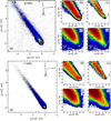 |
Fig. 1 Comet C/2014 A4 (SONEAR) in the g-sdss filter (top panel) and r-sdss filter (bottom panel), obtained at the BTA/SCORPIO-2. (a) direct images of the comet in relative intensity; (b) relative intensity image processed using the division by the 1/ρ profile method (Samarasinha & Larson 2014); (c) image processed by a rotational gradient method (Larson & Sekanina 1984); (d and e) relative intensity images to which a division by azimuthal average and renormalization methods were applied, respectively (Samarasinha & Larson 2014). The relative intensities of adjacent contours of isophotes differ by a factor of
|


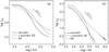 |
Fig. 2 Observed surface brightness profiles of comet C/2014 A4 (SONEAR) for flux calibrated images acquired in g-sdss (a) and r-sdss (b) bands. The individual curves are the scans taken through the photometric center in different directions. |
Radial slopes of profiles, in a log–log scale, measured in the g-sdss and r-sdss images of comet C/2014 A4 (SONEAR) at different ranges of coma distances.
3.4 Spectra
Cometary spectra consist of a continuum caused by the scattering of sunlight by dust particles and emissions due to the reemitting of the solar radiation by molecules in the cometary coma. We used a high-resolution solar spectrum (Neckel & Labs 1984) to separate these components. The solar spectrum was transformed to the resolution of our observations by convolving with the appropriate instrumental profile and normalized to the flux from the comet. Figure 5 shows step-by-stepprocessing of the comet C/2014 A4 spectrum. The convolved solar spectrum is compared with the cometary spectrum in Fig. 5a. We multiplied the solar spectrum by a polynomial (Fig. 5b). Subtracting the calculated continuum from the observed spectrum, we obtained a pure emission spectrum (Fig. 5c) that does not show any emission features.
We determined the upper limits to the emission fluxes of CN, C3, C2, and CO+, and upper limits to their (excluding CO+) production rates. For this, we adopted a Gaussian function having a FWHM equal to the spectral resolution as an equivalent of the minimum measurable signal. The amplitude of the Gaussian was equal to the RMS noise level calculated within wavelength regions associated with the bandpass of the narrowband cometary filters (Farnham et al. 2000). The Haser model (Haser 1957) was used to derive the upper limits to the production rates of the neutrals. The model parameters were taken from Langland-Shula & Smith (2011). The upper limits to the fluxes (F) and gas production rates (Q) are listed in Table 3. These values were computed with aperture of 1.56′′.
We also investigated variations in the reflectivity S(λ) along the dispersion expressed as the comet spectrum Fcom(λ) divided by the scaled solar spectrum: Fsun(λ): S(λ) = Fcom(λ)∕Fsun(λ). We used the polynomial from Fig. 5b to derive the dust reflectivity. The result shows a growth in dust reflectivity with increasing wavelength and can be presented quantitatively as the normalized gradient of reflectivity using the following expression (A’Hearn et al. 1984)
 (2)
(2)
where S(λ2) and S(λ1) correspond to the measurements at the wavelengths λ1 and λ2 (in Å) with λ2 > λ1, and S′(λ1, λ2) is expressed in percent per 1000 Å. With the adopted first degree of the polynomial fitting, the derived reddening is equal to 21.6 ± 0.2% per 1000 Å and is valid for the whole examined wavelength region: 4650–6200 Å. For comparison, Storrs et al. (1992) obtained the mean value of about 22% per 1000 Å (with the minimum and maximum values of 15% per 1000 Å and 37% per 1000 Å, respectively) within the 4400–5600 Å wavelength region for 18 ecliptic comets. For dynamically new distant comets, Kulyk et al. (2018) obtained rather different results: the normalized gradient of reflectivity was about 12% per 1000 Å and about 7% per 1000 Å for BV and VR spectral regions, respectively. Thus, the color of comet C/2014 A4 is comparable with that of ecliptic comets, but significantly redder than that of the distant comets studied by Kulyk et al. (2018). To find out a reason for this difference, a systematic study of the color of distant comets is required, especially because the color of comets may change significantly even on a daily basis (see Fig. 2 in Kolokolova et al. 2004; Ivanova et al. 2017b; Luk’yanyk et al. 2019).
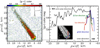 |
Fig. 3 Color map (g–r) of comet C/2014 A4 (SONEAR) derived from the November 5.85, 2015, images in the g-sdss and r-sdss filters (left). The map is color-coded according to the color indexes in magnitudes, as indicated at the top of the left image. The scans across the color map are displayed on the right: along the solar and anti-solar directions; perpendicular to the solar–anti-solar direction, and along and perpendicular to the tail. Positive distance is in the antisolar direction, and negative distance is in the solar direction. The inset shows a larger scale near-nucleus area with the directions of the scans. The vertical dashed lines indicate the spatial extent associated with the seeing. North, east, sunward, and velocity vector directions are indicated. |
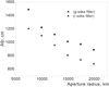 |
Fig. 4 Parameter Afρ vs. aperture radius measured in comet C/2014 A4 (SONEAR) trough the g-sdss and r-sdss filters with the BTA telescope. |
3.5 Polarimetry
The map ofpolarization degree for comet C/2014 A4, obtained in the broadband R (λ6420/790 Å) filter at the 6 m telescope, is presented in Fig. 6a. A fan-shaped region towards the Sun, also observed in photometricimages (Fig. 1), has a higher polarization then the surrounding coma. It seems that there is alsoa structure with a lower polarization extending from the near-nucleus region in the direction of the tail.
Figure 7 shows the observed radial profiles of polarization across the coma in the solar and perpendicularly to the solar–anti-solar directions and in the tail direction. Measurements of the polarization were performed with a 3 × 3 px size aperture along the selected directions in the coma. The maximum degree of polarization along the tail and perpendicular to the sunwarddirection was shifted relative to the photometric center toward the tail.
As can be seen in Fig. 7, there are significant differences in the radial profiles of polarization along the tail, in the solar direction, and perpendicular to the solar direction. In the near-nucleus region, ±10 000 km from the optocenter, all profiles display polarization variations within the range from −2.5 to −3.5%. At the distances 10 000–20 000 km, the polarization dropped sharply (by absolute value), from approximately −3.7 to −1.5%. Then, the degree of polarization increases gradually, although with different gradients, reaching about –5% at cometocentric distance 60 000 km in the solar direction and –8% at about 170 000 km in the tail. We note that the changes in polarization are not symmetrical relative to the photometric center.
The absolute values of the linear polarization for comet C/2014 A4 are significantly higher than those ever observed in the comets at heliocentric distances of less than 2 au where typical values do not exceed 2% (Kiselev et al. 2015). Our previous observationsof distant comets C/2010 S1 (LINEAR), C/2010 R1 (LINEAR), C/2011 KP36 (SPASEWATCH), C/2012 J1 (CATALINA), and C/2013 V4 (CATALINA) (Ivanova et al. 2015a; Ivanova & Afanasiev 2017) also showed the negative polarization degree whose absolute values changed with the distance from the nucleus from approximately −1.5 to −8%.
The distribution of the polarization vector (Fig. 6b) does not indicate any alignment of the dust particles. On average, the polarization vector is approximately PA = 80 ± 4°, i.e. practically parallel to the scattering plane (ϕ = 85°). This orientation of the polarization plane is typical in the case of negative polarization, i.e. for the light scattered by dust at the phase angles <20°.
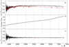 |
Fig. 5 Results of processing the spectrum of comet C/2014 A4 (SONEAR): (a) energy distribution in the observed cometary spectrum (black line) and the normalized spectrum of the Sun (red line); (b) normalized spectral dependence of the dust reflectivity; and (c) emission component in the cometary spectrum. |
Upper limits for the main emissions in comet C/2014 A4 (SONEAR).
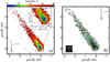 |
Fig. 6 Distribution of linear polarization degree (a) and polarization vectors (b) over the comet C/2014 A4 (SONEAR) coma derived through the R filter. The polarization (in percent) is color-coded (see scale bar above the left-hand image). The location of the optocenter is indicated with a white cross. The orientation of the vectors gives the direction of the local polarization plane, and the length of the vectors the degree of polarization. The projected directions toward the Sun, north, east, and comet velocity vector (V) are indicated. |
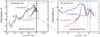 |
Fig. 7 Radial profiles of polarization across the coma of comet C/2014 A4 (SONEAR). Left: full polarization profiles, right: profiles for the near-nucleus area defined by the dashed rectangle. The vertical dotted lines indicate the seeing size. |
Complex refractive index of the materials considered in this study.
4 Modeling of variations of polarization and color over the coma
To interpretthe observational data, we used the rough spheroids model described in Kolokolova et al. (2015). There we found that the model can provide a good fit to the photopolarimetric observational data for comets using realistic characteristics of the dust particles. The rough spheroids model represents the dust as a polydisperse ensemble of spheroids with a range of aspect ratios. Roughness is presented by a normal distribution of the surface slopes, and is defined by the standard deviation of the distribution, which is zero for a smooth surface and greater than zero for a rough surface. A great advantage of the model is that there is a library of pre-calculated kernels for computations of the light scattering characteristics of rough spheroids (Dubovik et al. 2006), which can quickly provide brightness and polarization values for a variety of dust compositions, size distributions, and spheroid shapes.
4.1 Properties of the particles producing the observed negative polarization and red color
Based on the best fit for the cometary data obtained in Kolokolova et al. (2015), we selected a log-normal size distribution of particles with the effective variance veff = 0.1 and the range of aspect ratios of spheroids from 0.3 to 3, thus, covering both prolate and oblate spheroids. We described the spheroid roughness by the standard deviation σ = 0.2 that was the maximum roughness available in the pre-calculated kernels. The refractive indexes m for the materials considered in this study are listed in Table 4. There Halley-like dust represents a composition that was found typical for comet 1P/Halley dust particles based on Giotto mass-spectrometer data (Jessberger et al. 1988). We note that now we have new data on the composition of cometary dust resulted from the Rosetta studies of comet 67P/Churyumov-Gerasimenko (Bardyn et al. 2017), these data do not affect the refractive index of the dust substantially, and our computations show that the light scattering characteristics of the 1P/Halley and 67P/Churyumov-Gerasimenko dust look almost identical (Kolokolova & Kimura 2018).
Based on the success of modeling cometary photopolarimetric data in Kolokolova & Kimura (2010) and Kolokolova et al. (2015), we started with the same model as in those papers, i.e. we considered cometary dust as a mixture of porous Halley-dust and solid silicate particles. Although this model allows us to correctly reproduce the regular polarization phase curve and color (Fig. 8) and, for some size distributions, to reach negative polarization as low as −11% at phase angles ~15–18°, with this composition of cometary dust we could not reach polarization smaller than −0.3% at phase angle ~4° for the size distributions of any effective radius of particles. Numerous simulations for this mixture showed that changing parameters of the size distributions or considering Halley dust of different porosity or containing different silicates from Table 4 did not improve the results. Adding carbon or organics only worsens the situation as those absorptive materials led to vanishing negative polarization.
We accomplished computer simulations of polarization and color for the materials listed in Table 4. Our results showed that none of the absorbing materials (imaginary part of the refractive index > 0.1) produced a negative polarization. Thus, to reproduce the observed negative polarization, we needed some transparent material, i.e. a material with a low imaginary part of the refractive index. Our modeling for the silicates presented in Table 3 did not show negative polarization more negative than −0.7% at phase angle 4°. In addition, it was hard to imagine a comet with dust made of pure silicates. The most applicable candidate for the comets observed at large heliocentric distances is water ice, and our computations showed that particles made of pure water ice produce polarization about −3% at 4°. The lowest polarization at 4° was achieved for porous ice with porosity 55% (Fig. 9a) whose refractive index was calculated for a mixture of ice and voids using the Maxwell Garnett mixing rule. However, this and any other porous or solid ice showed a very blue color (Fig. 9b) at small phase angles. We also tried carbon dioxide ice and obtained similar results. However, since carbon dioxide was not detected in comet C/2014 A4 by NEOWISE observations (Bauer, priv. comm.), we continued our modeling using water ice.
To reproduce the observed red color, we needed a very red material, whose redness could overpower the blue color of ice. However, this material should not produce a significant positive polarization that might cancel the ice negative polarization, i.e. it should have a low imaginary part of the refractive index. After numerous attempts, we found that these characteristics were typical of tholins, and our computations showed (Fig. 10) that Titan’s tholin had the necessary photopolarimetric properties for particles larger than 1 μm. Tholins as acomponent of cometary material has already been considered in a number of publications starting from pioneering papers by Sagan & Khare (1979, and other papers by these authors) to the papers related to the interpretation of the Rosetta data (e.g. Stern et al. 2015; Poch et al. 2016; Frattin et al. 2019). In addition, Bonnet et al. (2015) showed that insoluble organic matter (IOM) found in carbonaceous meteorites and also considered as the organic component in the Rosetta dust (Bardyn et al. 2017) could originate from tholin-like organics. Although tholin in comets may not be identical to Titan’s tholin, we have found that the spectral properties of Titan’s tholin are similar to those of other tholins (e.g. Triton; see McDonald et al. 1994), and Titan’s tholin is the only type with reliably measured optical constants; it has been used in many papers to interpret cometary data, including that from Rosetta (see references above). We also performed computations for tholin ice, and the results were very similar to Titan’s tholin, which is not surprising from the comparison of their refractive indexes in Table 4.
From Figs. 9 and 10, we can see that combining icy particles between 1.5 and 2 μm in size with tholin particles of size >2 μm, we can reach very negative values of polarization and red color. This combination may be unrealistic for the comets observed at the heliocentric distances of about 1 au; however, it appears quite reasonable for distances around 4 au where comet C/2014 A4 was observed.
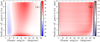 |
Fig. 8 Polarization degree (left) and (g–r) color (right) images computed for a mixture of porous Halley-like particles (porosity 85%) and solid silicate particles (forsterite); the ratio of the constituents in the mixture is 9:1. The figure demonstrates the applicability of the rough spheroid model to modeling polarization and color for regular (not distant) comets. Polarization is given in percent and color in magnitudes, but are calculated for the white-light illumination, i.e. they represent the intrinsic color of the dust or, from the astronomical point of view, the dust color excess. |
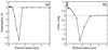 |
Fig. 9 Polarization (panel a) and (g–r) color (panel b) for ice of porosity 55% at phase angle 4°. Polarization was computed for r-sdss filter. Here we use the same definition of color as in Fig. 8, i.e. the presented values are intrinsic colors of the considered particles and are analogous to their color excess. |
Best-fit characteristics of the dust particles from our modeling.
4.2 Simulating the observed polarization and color trends in the coma
For a fair interpretation of our data, the characteristics of the dust particles in the tail should be consistent with the values of polarization and color observed near the nucleus. This means that the polarization should be around −2% and the color should be redder than in the tail, but the composition of the dust particles near the nucleus should be similar to the composition of the particles in the tail and the size of particles near the nucleus should be similar or larger since on the way to the tail particles can only evaporate, fragment, or be sorted by radiation pressure the way that small particles become more abundant in the tail.
An extensive analysis of all the data we obtained during our simulations with the goal of finding a behavior of the dust that can reproduce the values of polarization and the observed trends with realistic types of particles resulted in the following characteristics of the dust in comet C/2014 A4:
- 1.
Polarization in the tail, −8% can be achieved by a combination of tholin particles of radius >3 μm and porous icy particles of radius >0.75 μm (porosity30–50%) with the abundance of icy particles >98% in the mixture.
- 2.
Polarization in the non-tail directions, far from the nucleus, equal to −5%, needs tholin particles of radius >3 μm and porous icy particles of radius >1.0 μm (porosity ~30%). Abundance of icy particles should be 85–90% in the mixture.
- 3.
Polarization near the nucleus, −2.5%, can be reproduced by tholin particles of radius >3 μm, mixed with porous icy particles of radius <1.3 μm (porosity 30–50%). The larger the icy particles, the lower the abundance required. For example, icy particles of radius ~1 μm require 55% of them in the mixture, and even less for larger particles.
In Table 5, the solar color 0.44m was added to the calculated values of color to make them comparable with the observed that ranged from ~0.7 near the nucleus to ~0.4 in the tail; abundance means percent of the icy (or tholin) particles in the dust (i.e. it describes their contribution to the number density of particles). We can see that with our modeling we managed to reproduce the observed values of polarization and color, as well as their changes with the distance from the nucleus. The key result here is the combination of a very negative polarization with a very red color that was the main observational finding for this comet. We also successfully reproduced their significant change with the distance from the nucleus. Since the results were obtained with a rather simple model of rough spheroids, some small deviations from the observed values are not surprising. We note that adding a small amount of silicates (e.g. as a material underlying the tholin layer) can slightly decrease the color (making it even closer to the observed values) without affecting the values of polarization.
It may look doubtful that there was a smaller number of icy particles near the nucleus (e.g. 55%) than in the tail (>98%) if we assume that the particles can only change due to their sublimation. However, if we assume that the particles fragment on their way out of the nucleus, and in the case of the tail direction also sorted by radiation pressure, then we should expect that the number density of small icy particles increases with the distance from the nucleus. This can explain not only the smaller size of icy particles far from the nucleus, but also the larger abundance of icy particles there, especially in the tail. We note that the size of the tholin particles does not change; i.e. their abundance, relative to the icy particles, should decrease with distance.
The conclusion about the fragmentation of the particles in the coma is confirmed by our photometric data. For example, the decrease in Afρ with the distance from the nucleus (Fig. 4) most likely can be explained by the fragmentation of the particles because fragmentation causes a decrease in particle scattering cross section. We also see an indication of fragmentation in the radial profiles (Fig. 2). The profile curves are mostly steeper than 1/ρ, which confirms a decrease in particle size (see Sect. 3.2). Finally, we see a noticeable difference in the radial profiles for the r-sdss and g-sdss filters. Since the light scattering characteristics of particles change quickly when the particle size is comparable to the wavelength, this confirms the predominance of submicron- and micron-sized particles. We can probably claim that the particles size is close to 1 μm as the g-sdss filter profiles are usually flatter than r-sdss filter profiles, indicating that the particle fragmentation affects the r-sdss filter, whose wavelength is closer to 1 μm, stronger than the g-sdss filter. Thus, our photometric data are in good agreement with the results of our modeling.
5 Conclusions
We present the results of photometric, spectroscopic, and polarimetric observations of distant comet C/2014 A4 (SONEAR) carried out at the 6 m (SAO RAS) and 0.4 m telescope (Kourovka observatory, Russia) on November 5–7, 2015. From the analysis of the spectral observations we did not detect any emissions at or above the 3σ level. We estimated an upper limit of the gas production rate in the comet for the main emissions (CN, C3, C2, and CO+), which for C2 is equal to 0.98 × 1024 mol s−1. The continuum shows a reddening effect with the normalized gradient of reflectivity (21.6 ± 0.2)% per 1000 Å within the 4650–6200 Å wavelength range. We characterized the dust production via Afρ=680 ± 18 cm in the r-sdss filter.
Most of our knowledge about the physical properties of cometary dust were obtained based on the observations of comets close to the Sun (less than 2 au). Also, it was considered that the nature of the dust particles presented in the cometary coma does not depend on the heliocentric distance (Dollfus et al. 1988). However, new investigations show differences between the activity of comets close to the Sun and distant comets (see, e.g. Mazzotta Epifani et al. 2007, 2008; Ivanova et al. 2011, 2015b; Dlugach et al. 2018). Most likely the particles that form the comae are different. Ground-based polarimetric observations of distant comets had not been carried out until recently. The first detailed analysis of distribution of linear polarization in cometary coma for distant comets, with perihelion more than 4 au, were published by Ivanova et al. (2015a,c). Our results for comet C/2014 A4 support these results, which show a deeper branch of negative polarization at small phase angles in comparison with that observed for comets close to the Sun. The only case of a large negative polarization equal to −6% was reported by Hadamcik & Levasseur-Regourd (2003) for the circumnucleus halos of comets 81P/Wild 2 and 22P/Kopff. However, these comets were observed at phase angles of 9.7 and 18°, and at these phase angles polarization can reach very negative values even for a rather regular composition of the dust (see Fig. 8). Hines et al. (2014) found that the average (negative) polarization over the coma was −1.6% for the comet C/2012 S1 (ISON) at heliocentric distances 3.81 au. Such negative polarization is unusually low in comparison with that observed in other distant comets, and is perhaps related to the dynamical uniqueness of comet C/2012 S1 (ISON), which ended up as a sungrazing comet. In our observations of comet C/2014 A4, the polarization map shows spatial variations in the degree of polarization over the coma from about −3% near the nucleus to almost −8% in the tail. Analysis of the polarization and color and their change with the distance from the nucleus shows that (1) dust particles in the distant comets are small (<1 μm), which is not surprising as there is too little gas that can lift large particles; (2) dust contains icy particles and particles composed of (or covered by) tholin or similar organics; and (3) icy particles fragment as they move out of the nucleus. The photometric characteristics are consistent with the submicron/micron size of particles and the fragmentation of the dust particles in the coma.
Thus, our results suggest that the dust in distant comets differs from the dust in regular comets in both size and composition. For the regular comets, usually rather large particles made of a mixture of dark Halley-like material and silicates provide the best fit (Kiselev et al. 2015). For the case of distant comet C/2014 A4, we find that the dust particles are in the submicron-micron size range and their composition is characterized by a high abundance of ice and tholin-like organics. These characteristics of the dust in distant comets are quit realistic; far from the Sun we cannot expect that the sublimating gases will be able to lift particles that are as large as those lifted near the Sun. We can also expect that tholin is transformed close to the Sun, as described in Bonnet et al. (2015), for example.
Our results show how much more information can be extracted from observational data if we analyze photometricand polarimetric data together, especially combining polarization and color. Also, we enhance our understanding of the evolution of the dust in the coma if the analysis of polarization and color is complemented by studying variations of other photometric characteristics of the dust, specifically its radial profiles and change in Afρ with the distancefrom the nucleus.
Acknowledgements
The observations at the 6 m BTA telescope were performed with the financial support of the Ministry of Education and Science of the Russian Federation (agreement No. 14.619.21.0004, project ID RFMEFI61914X0004). O.I. thanks the SASPRO Programme No. 1287/03/01 for financial support. The research leading to these results has received funding from the People Programme (Marie Curie Actions) European Union’s Seventh Q12 Framework Programme under REA grant agreement No. 609427. Research has been further co-funded by the Slovak Academy of Sciences grant VEGA 2/0023/18. I.L. thanks the SAIA Programme for financial support. The research by O.I., I.L., and V.R. are supported, in part, by the project 19BF023-02 of the Taras Shevchenko National University of Kyiv. H.S.D. would like to acknowledge SERB, India, for funding a travel grant to UMD for collaborative work. We thank Ivan Mamoutike and Lennard Poliakov who analyzed the modeling data and compared them with the observations. We thank the C.A.R.A. project, and personally Gianantony Milani, Mauro Facchini (Cavezzo Observatory and Celado Observatory), and Rolando Ligustri (CAST) for providing their unpublished Afρ data for comet C/2014 A4 (SONEAR) for use in our manuscript. We thank Ivan Mamoutike and Lennard Poliakov who analyzed the modeling data and compared them with the observations.
References
- Afanasiev, V. L., & Amirkhanyan, V. R. 2012, Astrophys. Bull., 67, 438 [NASA ADS] [CrossRef] [Google Scholar]
- Afanasiev, V. L., & Moiseev, A. V. 2011, Balt. Astron., 20, 363 [NASA ADS] [Google Scholar]
- Afanasiev, V. L., Rosenbush, V. K., & Kiselev, N. N. 2014, Astrophys. Bull., 69, 211 [NASA ADS] [CrossRef] [Google Scholar]
- A’Hearn, M. F., Schleicher, D. G., Millis, R. L., Feldman, P. D., & Thompson, D. T. 1984, AJ, 89, 579 [NASA ADS] [CrossRef] [Google Scholar]
- A’Hearn, M. F., Feaga, L. M., Keller, H. U., et al. 2012, ApJ, 758, 29 [NASA ADS] [CrossRef] [Google Scholar]
- Bardyn, A., Baklouti, D., Cottin, H., et al. 2017, MNRAS, 469, S712 [CrossRef] [Google Scholar]
- Belton, M. J. S. 1965, AJ, 70, 451 [NASA ADS] [CrossRef] [Google Scholar]
- Bonnet, J.-Y., Quirico, E., Buch, A., et al. 2015, Icarus, 250, 53 [NASA ADS] [CrossRef] [Google Scholar]
- Capria, M. T., Coradini, A., & de Sanctis, M. C. 2002, Earth Moon Planets, 90, 217 [NASA ADS] [CrossRef] [Google Scholar]
- Dlugach, J. M., Ivanova, O. V., Mishchenko, M. I., & Afanasiev, V. L. 2018, J. Quant. Spectr. Rad. Transf., 205, 80 [NASA ADS] [CrossRef] [Google Scholar]
- Dollfus, A., Bastien, P., Le Borgne, J.-F., Levasseur-Regourd, A. C., & Mukai, T. 1988, A&A, 206, 348 [NASA ADS] [Google Scholar]
- Dones, L., Weissman, P. R., Levison, H. F., & Duncan, M. J. 2004, Star Formation in the Interstellar Medium: In Honor of David Hollenbach, ASP Conf. Ser., 323, 371 [NASA ADS] [Google Scholar]
- Dones, L., Brasser, R., Kaib, N., & Rickman, H. 2015, Space Sci. Rev., 197, 191 [NASA ADS] [CrossRef] [Google Scholar]
- Dorschner, J., Begemann, B., Henning, T., Jaeger, C., & Mutschke, H. 1995, A&A, 300, 503 [Google Scholar]
- Dubovik, O., Sinyuk, A., Lapyonok, T., et al. 2006, J. Geophys. Res. Atm., 111, D11208 [NASA ADS] [CrossRef] [Google Scholar]
- Egan, W. G., & Hilgeman, T. 1977, Icarus, 30, 413 [NASA ADS] [CrossRef] [Google Scholar]
- Eicher, D. J., & Levy, D. H. 2013, COMETS (Cambridge, UK: Cambridge University Press) [CrossRef] [Google Scholar]
- Fabian, D., Henning, T., Jäger, C., et al. 2001, A&A, 378, 228 [NASA ADS] [CrossRef] [EDP Sciences] [MathSciNet] [Google Scholar]
- Farnham, T. L., Schleicher, D. G., & A’Hearn, M. F. 2000, Icarus, 147, 180 [NASA ADS] [CrossRef] [Google Scholar]
- Frattin, E., Muñoz, O., Moreno, F., et al. 2019, MNRAS, 484, 2198 [NASA ADS] [CrossRef] [Google Scholar]
- Hadamcik, E., & Levasseur-Regourd, A. C. 2003, J. Quant. Spectr. Rad. Transf., 79, 661 [NASA ADS] [CrossRef] [Google Scholar]
- Haser, L. 1957, Bull. Soc. Roy. Sci. Liège, 43, 740 [Google Scholar]
- Heiles, C. 2000, AJ, 119, 923 [NASA ADS] [CrossRef] [Google Scholar]
- Hines, D. C., Videen, G., Zubko, E., et al. 2014, ApJ, 780, L32 [NASA ADS] [CrossRef] [Google Scholar]
- Hsu, J.-C., & Breger, M. 1982, ApJ, 262, 732 [NASA ADS] [CrossRef] [Google Scholar]
- Ivanova, O., & Afanasiev, V. 2017, European Planetary Science Congress, 11, EPSC2017-101 [Google Scholar]
- Ivanova, A. V., Korsun, P. P., & Afanasiev, V. L. 2009, Sol. Syst. Res., 43, 453 [NASA ADS] [CrossRef] [Google Scholar]
- Ivanova, O. V., Skorov, Y. V., Korsun, P. P., Afanasiev, V. L., & Blum, J. 2011, Icarus, 211, 559 [NASA ADS] [CrossRef] [Google Scholar]
- Ivanova, O. V., Dlugach, J. M., Afanasiev, V. L., Reshetnyk, V. M., & Korsun, P. P. 2015a, Planet. Space Sci., 118, 199 [NASA ADS] [CrossRef] [Google Scholar]
- Ivanova, O., Neslušan, L., Krišandová, Z. S., et al. 2015b, Icarus, 258, 28 [NASA ADS] [CrossRef] [Google Scholar]
- Ivanova, O., Shubina, O., Moiseev, A., & Afanasiev, V. 2015c, Astrophys. Bull., 70, 349 [NASA ADS] [CrossRef] [Google Scholar]
- Ivanova, O. V., Luk‘yanyk, I. V., Kiselev, N. N., et al. 2016, Planet. Space Sci., 121, 10 [NASA ADS] [CrossRef] [Google Scholar]
- Ivanova, O., Rosenbush, V., Afanasiev, V., & Kiselev, N. 2017a, Icarus, 284, 167 [NASA ADS] [CrossRef] [Google Scholar]
- Ivanova, O., Zubko, E., Videen, G., et al. 2017b, MNRAS, 469, 2695 [NASA ADS] [CrossRef] [Google Scholar]
- Ivanova, O., Reshetnyk, V., Skorov, Y., et al. 2018, Icarus, 313, 1 [NASA ADS] [CrossRef] [Google Scholar]
- Jessberger, E. K., Christoforidis, A., & Kissel, J. 1988, Nature, 332, 691 [NASA ADS] [CrossRef] [Google Scholar]
- Jewitt, D. 2015, AJ, 150, 201 [NASA ADS] [CrossRef] [Google Scholar]
- Jewitt, D., Agarwal, J., Hui, M.-T., et al. 2019, AJ, 157, 65 [NASA ADS] [CrossRef] [Google Scholar]
- Kartasheva, T. A., & Chunakova, N. M. 1978, Astrofizicheskie Issledovaniia Izvestiya Spetsial’noj Astrofizicheskoj Observatorii, 10, 44 [NASA ADS] [Google Scholar]
- Khare, B. N., Thompson, W. R., Cheng, L., et al. 1993, Icarus, 103, 290 [NASA ADS] [CrossRef] [Google Scholar]
- Kimura, H., Kolokolova, L., & Mann, I. 2003, A&A, 407, L5 [NASA ADS] [CrossRef] [EDP Sciences] [Google Scholar]
- Kiselev, N., Rosenbush, V., Levasseur-Regourd, A.-C., & Kolokolova, L. 2015, Polarimetry of Stars and Planetary Systems (Cambridge, UK: Cambridge University Press), 379 [Google Scholar]
- Kolokolova, L., & Kimura, H. 2010, Earth Planets, Space, 62, 17 [NASA ADS] [CrossRef] [Google Scholar]
- Kolokolova, L., & Kimura, H., 2018 New challenges for cometary dust modeling after Rosetta, presented at “Physics of comets after the Rosetta mission: Unresolved problems”, September 5–7, 2018, Stara Lesna, Slovakia, https://www.astro.sk/AFTERROSETTA/wp-content/uploads/2018/10/Kolokolova.pdf [Google Scholar]
- Kolokolova, L., Hanner, M. S., Levasseur-Regourd, A.-C., & Gustafson, B. Å. S. 2004, Comets II (Tucson: University of Arizona), 577 [Google Scholar]
- Kolokolova, L., Das, H. S., Dubovik, O., Lapyonok, T., & Yang, P. 2015, Planet. Space Sci., 116, 30 [NASA ADS] [CrossRef] [Google Scholar]
- Korsun, P. P., & Chörny, G. F. 2003, A&A, 410, 1029 [NASA ADS] [CrossRef] [EDP Sciences] [Google Scholar]
- Korsun, P. P., Ivanova, O. V., & Afanasiev, V. L. 2006, A&A, 459, 977 [NASA ADS] [CrossRef] [EDP Sciences] [Google Scholar]
- Korsun, P. P., Ivanova, O. V., & Afanasiev, V. L. 2008, Icarus, 198, 465 [NASA ADS] [CrossRef] [Google Scholar]
- Kulyk, I., Rousselot, P., Korsun, P. P., et al. 2018, A&A, 611, A32 [NASA ADS] [CrossRef] [EDP Sciences] [Google Scholar]
- Langland-Shula, L. E., & Smith, G. H. 2011, Icarus, 213, 280 [CrossRef] [Google Scholar]
- Larson, S. M., & Sekanina, Z. 1984, AJ, 89, 571 [NASA ADS] [CrossRef] [Google Scholar]
- Levison, H. F., Morbidelli, A., Van Laerhoven, C., Gomes, R., & Tsiganis, K. 2008, Icarus, 196, 258 [NASA ADS] [CrossRef] [Google Scholar]
- Levison, H. F., Duncan, M. J., Brasser, R., & Kaufmann, D. E. 2010, Science, 329, 187 [NASA ADS] [CrossRef] [Google Scholar]
- Li, A., & Greenberg, J. M. 1997, A&A, 323, 566 [NASA ADS] [Google Scholar]
- Luk’yanyk, I., Zubko, E., Husárik, M., et al. 2019, MNRAS, 485, 4013 [NASA ADS] [CrossRef] [Google Scholar]
- McDonald, G. D., Thompson, W. R., Heinrich, M., Khare, B. N., & Sagan, C. 1994, Icarus, 108, 137 [NASA ADS] [CrossRef] [Google Scholar]
- Mandt, K. E., Mousis, O., Marty, B., et al. 2015, Space Sci. Rev., 197, 297 [NASA ADS] [CrossRef] [Google Scholar]
- Mazzotta Epifani, E., Palumbo, P., Capria, M. T., et al. 2007, MNRAS, 381, 713 [NASA ADS] [CrossRef] [Google Scholar]
- Mazzotta Epifani, E., Palumbo, P., Capria, M. T., et al. 2008, MNRAS, 390, 265 [NASA ADS] [CrossRef] [Google Scholar]
- Mazzotta Epifani, E., Perna, D., Licandro, J., et al. 2014, A&A, 565, A6 [NASA ADS] [CrossRef] [EDP Sciences] [Google Scholar]
- Meech, K. J., Pittichová, J., Bar-Nun, A., et al. 2009, Icarus, 201, 719 [NASA ADS] [CrossRef] [Google Scholar]
- Neckel, H., & Labs, D. 1984, Sol. Phys., 90, 205 [NASA ADS] [CrossRef] [Google Scholar]
- Nesvorný, D., Vokrouhlický, D., Dones, L., et al. 2017, ApJ, 845, 27 [NASA ADS] [CrossRef] [Google Scholar]
- Oke, J. B. 1990, AJ, 99, 1621 [NASA ADS] [CrossRef] [Google Scholar]
- Ootsubo, T., Kawakita, H., Hamada, S., et al. 2012, ApJ, 752, 15 [NASA ADS] [CrossRef] [Google Scholar]
- Picazzio, E., Luk’yanyk, I. V., Ivanova, O. V., et al. 2019, Icarus, 319, 58 [NASA ADS] [CrossRef] [Google Scholar]
- Poch, O., Pommerol, A., Jost, B., et al. 2016, Icarus, 267, 154 [NASA ADS] [CrossRef] [Google Scholar]
- Prialnik, D. 1992, ApJ, 388, 196 [NASA ADS] [CrossRef] [Google Scholar]
- Ramirez, S. I., Coll, P., da Silva, A., et al. 2002, Icarus, 156, 515 [NASA ADS] [CrossRef] [Google Scholar]
- Roemer, E. 1962, PASP, 74, 537 [NASA ADS] [CrossRef] [Google Scholar]
- Rosenbush, V. K., Ivanova, O. V., Kiselev, N. N., Kolokolova, L. O., & Afanasiev, V. L. 2017, MNRAS, 469, S475 [CrossRef] [Google Scholar]
- Rouleau, F., & Martin, P. G. 1991, ApJ, 377, 526 [NASA ADS] [CrossRef] [Google Scholar]
- Sagan, C., & Khare, B. N. 1979, Nature, 281, 708 [NASA ADS] [CrossRef] [Google Scholar]
- Samarasinha, N. H., & Larson, S. M. 2014, Icarus, 239, 168 [NASA ADS] [CrossRef] [Google Scholar]
- Sárneczky, K., Szabó, G. M., Csák, B., et al. 2016, AJ, 152, 220 [NASA ADS] [CrossRef] [Google Scholar]
- Schmidt, G. D., Elston, R., & Lupie, O. L. 1992, AJ, 104, 1563 [NASA ADS] [CrossRef] [Google Scholar]
- Scott, A., & Duley, W. W. 1996, ApJS, 105, 401 [NASA ADS] [CrossRef] [Google Scholar]
- Solontoi, M., Ivezić, Ž., Jurić, M., et al. 2012, Icarus, 218, 571 [NASA ADS] [CrossRef] [Google Scholar]
- Stansberry, J. A., Van Cleve, J., Reach, W. T., et al. 2004, ApJS, 154, 463 [NASA ADS] [CrossRef] [Google Scholar]
- Stern, S. A., Feaga, L. M., Schindhelm, E., et al. 2015, Icarus, 256, 117 [NASA ADS] [CrossRef] [Google Scholar]
- Storrs, A. D., Cochran, A. L., & Barker, E. S. 1992, Icarus, 98, 163 [NASA ADS] [CrossRef] [Google Scholar]
- Trigo-Rodríguez, J. M., García-Melendo, E., Davidsson, B. J. R., et al. 2008, A&A, 485, 599 [NASA ADS] [CrossRef] [EDP Sciences] [Google Scholar]
- Warren, S. G. 1984, Appl. Opt., 23, 1206 [NASA ADS] [CrossRef] [PubMed] [Google Scholar]
- Warren, S. G. 1986, Appl. Opt., 25, 2650 [NASA ADS] [CrossRef] [Google Scholar]
- Weissman, P. R. 1990, Nature, 344, 825 [NASA ADS] [CrossRef] [Google Scholar]
- Weissman, P. R. 1997, Ann. N. Y. Acad. Sci., 822, 67 [NASA ADS] [CrossRef] [Google Scholar]
- Williams, G.V., 2014. MPEC 2014-B03: Comet C/2014 A4 (SONEAR) [Google Scholar]
All Tables
Radial slopes of profiles, in a log–log scale, measured in the g-sdss and r-sdss images of comet C/2014 A4 (SONEAR) at different ranges of coma distances.
All Figures
|
Fig. 1 Comet C/2014 A4 (SONEAR) in the g-sdss filter (top panel) and r-sdss filter (bottom panel), obtained at the BTA/SCORPIO-2. (a) direct images of the comet in relative intensity; (b) relative intensity image processed using the division by the 1/ρ profile method (Samarasinha & Larson 2014); (c) image processed by a rotational gradient method (Larson & Sekanina 1984); (d and e) relative intensity images to which a division by azimuthal average and renormalization methods were applied, respectively (Samarasinha & Larson 2014). The relative intensities of adjacent contours of isophotes differ by a factor of
|
| In the text | |
|
Fig. 2 Observed surface brightness profiles of comet C/2014 A4 (SONEAR) for flux calibrated images acquired in g-sdss (a) and r-sdss (b) bands. The individual curves are the scans taken through the photometric center in different directions. |
| In the text | |
|
Fig. 3 Color map (g–r) of comet C/2014 A4 (SONEAR) derived from the November 5.85, 2015, images in the g-sdss and r-sdss filters (left). The map is color-coded according to the color indexes in magnitudes, as indicated at the top of the left image. The scans across the color map are displayed on the right: along the solar and anti-solar directions; perpendicular to the solar–anti-solar direction, and along and perpendicular to the tail. Positive distance is in the antisolar direction, and negative distance is in the solar direction. The inset shows a larger scale near-nucleus area with the directions of the scans. The vertical dashed lines indicate the spatial extent associated with the seeing. North, east, sunward, and velocity vector directions are indicated. |
| In the text | |
|
Fig. 4 Parameter Afρ vs. aperture radius measured in comet C/2014 A4 (SONEAR) trough the g-sdss and r-sdss filters with the BTA telescope. |
| In the text | |
|
Fig. 5 Results of processing the spectrum of comet C/2014 A4 (SONEAR): (a) energy distribution in the observed cometary spectrum (black line) and the normalized spectrum of the Sun (red line); (b) normalized spectral dependence of the dust reflectivity; and (c) emission component in the cometary spectrum. |
| In the text | |
|
Fig. 6 Distribution of linear polarization degree (a) and polarization vectors (b) over the comet C/2014 A4 (SONEAR) coma derived through the R filter. The polarization (in percent) is color-coded (see scale bar above the left-hand image). The location of the optocenter is indicated with a white cross. The orientation of the vectors gives the direction of the local polarization plane, and the length of the vectors the degree of polarization. The projected directions toward the Sun, north, east, and comet velocity vector (V) are indicated. |
| In the text | |
|
Fig. 7 Radial profiles of polarization across the coma of comet C/2014 A4 (SONEAR). Left: full polarization profiles, right: profiles for the near-nucleus area defined by the dashed rectangle. The vertical dotted lines indicate the seeing size. |
| In the text | |
|
Fig. 8 Polarization degree (left) and (g–r) color (right) images computed for a mixture of porous Halley-like particles (porosity 85%) and solid silicate particles (forsterite); the ratio of the constituents in the mixture is 9:1. The figure demonstrates the applicability of the rough spheroid model to modeling polarization and color for regular (not distant) comets. Polarization is given in percent and color in magnitudes, but are calculated for the white-light illumination, i.e. they represent the intrinsic color of the dust or, from the astronomical point of view, the dust color excess. |
| In the text | |
|
Fig. 9 Polarization (panel a) and (g–r) color (panel b) for ice of porosity 55% at phase angle 4°. Polarization was computed for r-sdss filter. Here we use the same definition of color as in Fig. 8, i.e. the presented values are intrinsic colors of the considered particles and are analogous to their color excess. |
| In the text | |
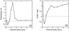 |
Fig. 10 Same as Fig. 9, but for Titan tholins. |
| In the text | |
Current usage metrics show cumulative count of Article Views (full-text article views including HTML views, PDF and ePub downloads, according to the available data) and Abstracts Views on Vision4Press platform.
Data correspond to usage on the plateform after 2015. The current usage metrics is available 48-96 hours after online publication and is updated daily on week days.
Initial download of the metrics may take a while.