| Issue |
A&A
Volume 626, June 2019
|
|
|---|---|---|
| Article Number | A17 | |
| Number of page(s) | 18 | |
| Section | Galactic structure, stellar clusters and populations | |
| DOI | https://doi.org/10.1051/0004-6361/201834957 | |
| Published online | 05 June 2019 | |
Expanding associations in the Vela-Puppis region
3D structure and kinematics of the young population⋆
1
Institut de Ciències del Cosmos, Universitat de Barcelona (IEEC-UB), Martí i Franquès 1, 08028 Barcelona, Spain
e-mail: This email address is being protected from spambots. You need JavaScript enabled to view it.
2
Astrophysics Group, Keele University, Keele ST5 5BG, UK
3
INAF, Osservatorio Astronomico di Padova, Vicolo Osservatorio 5, 35122 Padova, Italy
4
Institut für Astro- und Teilchenphysik, Universität Innsbruck, Technikerstrasse 25/8, 6020 Innsbruck, Austria
Received:
21
December
2018
Accepted:
18
April
2019
Abstract
Context. The Vela-Puppis region is known to host the Vela OB2 association as well as several young clusters featuring OB and pre-main-sequence stars. Several spatial and kinematic subgroups have been identified in recent years.
Aims. By grouping stars based on their positions and velocity, we can address the question of the dynamical history of the region and the mechanisms that drove stellar formation. The Gaia DR2 astrometry and photometry enables us to characterise the 3D spatial and 3D kinematic distribution of young stars and to estimate the ages of the identified components.
Methods. We used an unsupervised classification method to group stars based on their proper motions and parallax. We studied the expansion rates of the different identified groups based on 3D velocities and on corrected tangential velocities. We used theoretical isochrones to estimate ages.
Results. The young stars can be separated into seven main groups of different ages and kinematical distribution. All groups are found to be expanding, although the expansion is mostly not isotropic.
Conclusions. The size of the region, the age substructure, and the anisotropic expansion rates are compatible with a prolonged period of star formation in a turbulent molecular cloud. The current kinematics of the stars cannot be explained by internal processes alone (such as gas expulsion).
Key words: open clusters and associations: individual: Vela OB2 / open clusters and associations: individual: Trumpler 10 / open clusters and associations: individual: NGC 2547 / open clusters and associations: individual: NGC 2451B / stars: pre-main sequence
The list of members of the young populations established in this study is only available at the CDS via anonymous ftp to cdsarc.u-strasbg.fr (130.79.128.5) or via http://cdsarc.u-strasbg.fr/viz-bin/qcat?J/A+A/626/A17
© ESO 2019
1. Introduction
It has been known for a long time that O and B stars are not distributed randomly on the sky (Eddington 1910; Kapteyn 1914; Rasmuson 1921) and that they form sparse groups of co-moving stars. The term “association” was introduced by Ambartsumian (1947). Although OB associations are too sparsely populated to be gravitationally bound (Bok 1934; Mineur 1939), their internal velocity dispersion is small enough that they can be identified as overdensities in velocity space. While the historical name OB association is widely used in the literature, these groupings of young stars are known to include lower-mass stars and pre-main-sequence stars, following a continuous mass function (Briceño et al. 2007).
Significant progress in the description and characterisation of OB associations was made when the HIPPARCOS mission opened a new era in the study of the solar neighbourhood (e.g. Brown et al. 1997, 1999; Comeron et al. 1998; de Zeeuw et al. 1999; Hoogerwerf & Aguilar 1999; Kaltcheva & Hilditch 2000; Elias et al. 2006; Caballero & Dinis 2008; Bouy & Alves 2015) by providing parallaxes and precise proper motions for ∼100 000 stars, most of them brighter than G ∼ 12. More recently, the unprecedented quality of the astrometry provided by the second Gaia data release (Gaia DR2, Gaia Collaboration 2018b) has enabled detailed studies of the spatial and kinematic substructure of stellar associations within several hundreds of parsecs of the Sun (e.g. Kuhn et al. 2019; Kounkel et al. 2018; Damiani 2018; Karnath et al. 2019; Zari et al. 2018; Kos et al. 2018).
The Vela OB2 association was originally reported by Kapteyn (1914). The first description of its kinematics comes from de Zeeuw et al. (1999), who noted that the space motion of the association is not clearly separate from the surrounding stars and the nearby (slightly older) open clusters NGC 2547 and Trumpler 10. Pozzo et al. (2000) identified through X-ray observations a group of pre-main-sequence stars (PMS) that are located around the massive binary system γ2 Vel, which lies at a distance of 350–400 pc from us. This group of young stars (∼10 Myr, Jeffries et al. 2009), sometimes referred to as the Gamma Velorum cluster (or Pozzo 1 in Dias et al. 2002), has been the object of many recent publications. Making use of spectroscopic observations from the Gaia-ESO Survey (Gilmore et al. 2012; Randich et al. 2013; Jeffries et al. 2014), and Sacco et al. (2015) have shown that two kinematic groups exist in the region. In a subsequent study making use of N-body simulations, Mapelli et al. (2015) showed that the spatial and velocity distributions of these stars correspond to a supervirial spatially expanding structure.
Several further studies have been published since the release of the first Gaia catalogue (Gaia Collaboration 2016a,b). Using Gaia DR1 data astrometry, Damiani et al. (2017) noted that the proper motions of the stars located in a few degrees around γ2 Vel are mainly distributed in two groups of different age, with the significantly older one including NGC 2547. Franciosini et al. (2018) have shown that the kinematic populations identified from the Gaia-ESO Survey radial velocities also present distinct proper motions and parallaxes, and Beccari et al. (2018) noted that the region might host not two but at least four non-coeval kinematic groups, with a fragmented spatial distribution. Armstrong et al. (2018) studied the distribution of the stars coeval with the Gamma Velorum cluster, and compared it with the Vela OB2 stars of de Zeeuw et al. (1999), noting that the OB stars are not all located in high-density regions of young PMS stars. Finally, Cantat-Gaudin et al. (2019) identified 11 distinct groups in 3D positional and velocity space, spread over more than a hundred parsecs, and confirmed that their overall structure is expanding. The centre of this structure appears devoid of stars, and its projection on the sky matches the large bubble known as the IRAS Vela Shell (IVS, Sahu 1992). The authors suggested that feedback from a slightly older stellar population might have driven the formation of both the Vela OB2 stars and the IVS.
In this paper we make use of Gaia DR2 to study the 3D spatial and 3D velocity distribution of young stars over a large scale in the direction of the Vela and Puppis constellations. This paper is organised as follows: in Sect. 2 we describe our data selection, in Sect. 3 we characterise the observed radial and tangential velocity distributions, in Sect. 4 we derive ages for the different observed populations, and in Sect. 5 we provide individual comments on the different populations. Sect. 6 contains a discussion, and we conlcude in Sect. 7 with a summary of this study.
2. Data
We queried the Gaia-DR2 archive1 for stars brighter than G = 18 in a large field (31 ° ×20°) and in the parallax range ϖ ∈ [1.8, 4] mas (roughly corresponding to distances from 250 to 550 pc). This spatial selection includes the known clusters Trumpler 10, NGC 2451B, NGC 2547, Collinder 135, Collinder 140, UBC 7, and BH 23, as well as the extended Vela OB2 complex. The investigated region is shown in Fig. 1.
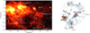 |
Fig. 1. Left: composite of an IRIS 60 μm image (Miville-Deschênes & Lagache 2005) and DSS optical image of the investigated region. Right: distribution of PMS stars projected on the Galactic plane from Zari et al. (2018). The radii of the concentric circles centred on the Sun increase from 100 to 500 pc. |
We followed Eqs. (1) (restriction on the astrometric unit-weight error, UWE) and (2) (on the photometric excess flux) from Arenou et al. (2018) in order to filter out the stars with poor astrometric solutions and poor photometry. This selection is slightly more permissive than the filter introduced by Lindegren (2018), who recommended to discard all sources with a re-normalised unit weight (RUWE) larger than 1.4. In the end (after applying the selections described in Sects. 2.1 and 2.2), we find that about 4% of our final sample has RUWE > 1.4, and 1% has RUWE > 2, while using the RUWE filter would introduce no additional sources. The stars with RUWE > 1.4 exhibit the same patterns in photometric, spatial, and velocity space as the rest of the sample (although often with larger astrometric uncertainties than stars at the same magnitude), and the results presented in this paper do not depend on the choice of filtering.
Throughout this paper we estimate distances to individual stars by inverting their parallax. Although this simple estimation is not recommended for the vast majority of the sources in the Gaia DR2 catalogue (see e.g. Bailer-Jones 2015; Luri et al. 2018), the stars we studied have typical fractional parallax uncertainties of 2% (and are all under 11%), which introduces only a negligible bias. All uncertainties on quantities derived from distances (such as absolute magnitude MG or tangential velocity v2) are estimated by propagating parallax uncertainties (using the covariance matrix between the astrometric measurements μα*, μδ, and ϖ).
We note  (if ϖ expressed in mas) the observed magnitude G corrected for distance, but not for extinction. We added a fixed correction of +0.029 mas to all Gaia DR2 parallaxes. This value corresponds to the parallax zero-point offset reported by Lindegren et al. (2018), and roughly corresponds to a 2 pc offset at a distance of 250 pc, or a 10 pc offset at a distance of 600 pc. We recall that because of the uncertainty on the true value of this zero-point (and its possible dependence on colour and magnitude, Arenou et al. 2018) and local systematics (Lindegren et al. 2018; Arenou et al. 2018; Vasiliev 2018), the uncertainty on the true absolute distance of a source is always larger than the uncertainty on its inverse parallax.
2.1. Photometric selection
We empirically devised a broad photometric selection that is intended to retain the younger stars while rejecting low-mass main-sequence stars and evolved stars where possible. The filter was built using the members of Trumpler 10, NGC 2451B, NGC 2547, Collinder 135, Collinder 140, and the Gamma Velorum cluster (Pozzo 1) as reference stars. The cluster member list for these objects was taken from Cantat-Gaudin et al. (2018a), who performed a selection based on astrometric criteria only.
We defined the blue edge of the filter as the 10th percentile of the GBP − GRP colour of the reference stars in sliding windows of 1 mag in MG, offset by −0.1 mag. The red edge of the filter was arbitrarily chosen to discard evolved stars. Figure 2 shows the location of the retained and discarded stars in a HR diagram. The filter discards about half the stars fainter than MG ∼ 7, and a third of the total sample.
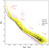 |
Fig. 2. Photometric selection of young stars. The reference stars are the members of the young clusters Trumpler 10, NGC 2451B, NGC 2547, Collinder 135, Collinder 140, and the Gamma Velorum cluster (Pozzo 1). The dashed line corresponds to the zero-age main sequence for a PARSEC isochrone of metallicity Z = 0.019 and AV = 0.15. |
2.2. Astrometric cleaning of the field stars using UPMASK
The Gaia DR2 astrometry allows us to identify groups of stars not solely as overdensities in positional space, but as sharing common proper motions (μα*,μδ) and parallaxes (ϖ) as well. In this study we applied the unsupervised classification scheme of UPMASK (Krone-Martins & Moitinho 2014). This approach does not rely on assumptions on the structure of a group of star in positional or in astrometric space, and only requires that stars with similar properties in astrometric space must occupy less space on the sky than a random uniform distribution (we call this step the veto). In our implementation (as in Cantat-Gaudin et al. 2018b), we used k-means clustering to define small groups of stars in astrometric space, and the total length of a minimum spanning tree (MST) to compare the spatial distribution of each group with a uniform distribution. We consider that a group of stars is clustered if the total branch length of its MST is shorter than the mean MST of a random distribution by at least 1σ.
We repeated the procedure 100 times, each time redrawing a new value for the proper motion and parallax of every star based on the full covariance matrix of its (μα*,μδ,ϖ) uncertainties. In a frequentist approach, the final score (how many times a star was part of a group that passed the veto) can be interpreted as a membership probability ranging from 0 to 100%.
The advantage of this approach is that we do not require groups to be spatially dense, but only that they occupy a smaller area than the whole field of view. This allowed us to retain elongated structures if they are made up of stars with similar proper motions and parallaxes. The approach is independent of the number of clusters present, as it only discards non-clustered stars. It is also entirely unsupervised and does not rely on a threshold density or a maximum distance between points in the parameter space (as in e.g. DBSCAN, Ester et al. 1996), which allowed us to find clusters of various densities, and to keep the low-density tails of the identified groups.
2.3. Splitting the sample into distinct populations
We verified that the stars with membership scores < 50% were uniformly distributed in the field of view and showed no obvious structure in proper motion space. In the rest of this study we only worked with the sample of stars with scores > 50%, whose proper motions (μα*,μδ), tangential velocities (vℓ,vb), and positions (ℓ,b) are shown in Fig. 3.
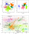 |
Fig. 3. Top left: proper motions of the stars with UPMASK clustering scores larger than 50%. Top right: tangential velocities (in Galactic coordinates) of the same stars. The colours correspond to the seven populations defined from their tangential velocities (see text). Bottom: spatial distribution of the same stars. |
The distribution in proper motion space is partly shaped by the fragmented spatial distribution of the stars, and their distribution in tangential velocity space (accounting for the individual parallax of each star) appears more compact, as shown in Fig. 3. From Monte Carlo propagation of the Gaia DR2 uncertainty on the proper motions and parallaxes, we find the typical uncertainty in tangential velocity to be ∼0.3 km s−1.
We identified seven main groups in (vℓ,vb) space, showing very little overlap. We labelled these groups from population I to population VII (in order of decreasing age, as later estimated in Sect. 4). Their distributions on the sky (ℓ,b) and on the plane of the Milky Way (X,Y) are shown in Figs. A.1–A.7.
We note that our sample includes a few upper main-sequence stars from the nearby (∼278 pc, Cantat-Gaudin et al. 2018a) older cluster Alessi 3 (log t of 8.7 and 8.87 in Dias et al. 2002; Kharchenko et al. 2013, respectively), which is located less than half a degree outside of the southern boundary of the investigated region. These stars can easily be discarded based on their tangential velocity and compact location on the sky.
We tried several approaches in order to provide the final division of the sample into seven populations. We found that the two methods that provide the most satisfying decomposition are (i) performing hard cuts in (vℓ,vb) and (μα*,μδ) space or (ii) agglomerative clustering (Müllner 2011). Gaussian mixture models or k-means clustering performed poorly on this dataset, overfitting the observed structure or grouping together stars with too different velocities. The division we adopted for the rest of this study was obtained from agglomerative clustering. We note that most stars were assigned the same population regardless of the method used, and that the choice of splitting method only concerns a small number of stars. We verified that the results and conclusions of this paper are identical whether supervised agglomerative clustering or purely manual splitting was performed. In particular, the velocities of the five clusters known as Collinder 135, Collinder 140, NGC 2451B, NGC 2547, and UBC 7 are similar enough for the clusters to always be classified as subgroups of the same main kinematic population.
3. Linear expansion rates
In this section we characterise the kinematic structure of the seven populations by establishing whether they exhibit a spatial velocity gradient. A positive correlation between the position along a given axis and the velocity along this axis is interpreted as evidence for expansion. The approach we follow is similar to that applied by Wright & Mamajek (2018) to the Scorpius-Centaurus association.
3.1. From 3D velocities
The most direct way to study the internal kinematics of a group of stars is to independently determine a 3D velocity vector for each member star. In practice, only 10% of the stars in our sample have Gaia DR2 radial velocities, with a typical uncertainty of 3.3 km s−1. Figure 4 shows the observed Gaia DR2 radial velocities as a function of line-of-sight distance for the seven populations. We estimated the uncertainty on the slope by Monte-Carlo redrawings of parallaxes and radial velocities of the Gaussian nominal uncertainties. The observed gradient is only significantly positive (by more than 2σ) for populations II and VII because of the relatively large nominal uncertainties on the radial velocities.
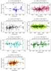 |
Fig. 4. Gaia DR2 radial velocity as a function of distance for the stars in each population identified in this study. κr: slope of the radial velocity gradient with distance (×10−2 km s−1 pc−1). μ: mean radial velocity (km s−1). σ: standard deviation (km s−1). σ/ |

We computed the position (X,Y,Z) in Galactic Cartesian coordinates for each member of each population, and its velocity vector (vX,vY,vZ) from its observed proper motions and radial velocity. For each component we discarded the stars whose velocity was discrepant from the sample mean by more than 3σ, then fit a linear relationship between X and vX (and similarly for the Y and Z axes). The slopes (κX, κY, and κZ) we obtained are listed in Table 1 and are shown in Fig. 5 (for the X and Z axes only). Because the investigated region is located near ℓ = 270°, the velocity component vY is roughly equivalent to the radial velocity and inherits its large uncertainty, while vX and vZ are better constrained.
Linear expansion rates.
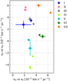 |
Fig. 5. Observed linear expansion rates (as listed in Table 1). Squares: (κX,κZ) from 3D velocities. Dots: (κℓ,κb) from corrected tangential velocities (see Sect. 3.2). The colour-coding is the same as in Figs. 3 and 4. |
We observe that all seven populations exhibit a significant positive correlation between X and vX (κX > 0). Most of them also exhibit signs of expansion along the Z axis (perpendicular to the Galactic plane), with the exception of population V, which exhibits no significant correlation, and population IV, whose velocity gradient κY appears negative. Rather than a sign of contraction, we argue that a simple linear expansion model is not appropriate to describe the internal kinematics of this group, which exhibits a complex substructure, and whose individual components would be better treated separately. We further discuss this population in Sect. 5. Overall, the only groups exhibiting an isotropic expansion (κX ≃ κZ) are populations I and III.
Following the formulation of Blaauw (1964) and Wright & Mamajek (2018), the slopes κ can also be expressed as an expansion age: τ = (γκ)−1 (where γ = 1.0227 is the conversion factor from km s−1 to pc Myr−1. Inverting this relation allows us to derive κ from an estimated age. We find that the observed κX (and κℓ) are slightly lower than expected from the ages derived in Sect. 4, but that they generally follow the expected trend, with the youngest (populations VII and VI) exhibiting the highest expansion rates and populations I and II the slowest.
3.2. From tangential velocities
The precision of the Gaia DR2 astrometry allows us to derive tangential velocities (vℓ,vb) with typical uncertainties under 0.3 km s−1 for a large number of stars. Because most of these stars lack a measurement of their radial velocity, the interpretation of these tangential velocities is not straightforward.
The observed proper motions (and inferred tangential velocities) of the stars that move away from us suffer from a perspective effect that introduces a virtual contraction (for a group of stars with negative radial velocity, a virtual expansion). If the bulk radial velocity of the group of stars is known, the effects of virtual contraction and of true physical contraction can be distinguished. When no physical expansion or contraction is assumed, the mean distance can be inferred from the radial velocity with the so-called moving cluster method (see e.g. Jones 1971; de Bruijne 1999). Alternatively, a mean radial velocity can be derived for a non-expanding cluster of known distance (e.g. Dravins et al. 1999). We corrected the tangential velocities (vℓ,vb) following Eq. (A3) of Brown et al. (1997). The corrected tangential velocities ( ,
, ) are
) are
![Mathematical equation: $$ \begin{aligned} \begin{split} { v}\prime _{\ell }&= { v}_{\ell } - { v}_{\rm rad} \cos b_{\rm c} \sin ( \ell _{\rm c} - \ell ) , \\ { v}\prime _{b}&= { v}_{b} - { v}_{\rm rad} \left[ \sin b_{\rm c} \cos b - \sin b \cos b_{\rm c} \cos \left( \ell _{\rm c} - \ell \right) \right] \end{split} ,\end{aligned} $$](/articles/aa/full_html/2019/06/aa34957-18/aa34957-18-eq5.gif) (1)
(1)
where (ℓc,bc) is the location of the centre of the distribution of each population, and vrad is the mean radial velocity. To a good approximation (ℓc − ℓ < 15°), virtual contraction introduces a linear expansion with angular distance from the distribution centre (see e.g. Blaauw 1952; Lesh 1968).
After applying the correction for virtual expansion using the mean radial velocities derived in Sect. 3.1, we find that all populations exhibit significant residual positive gradients of  with ℓ (and similarly of
  with b). We only illustrate the apparent and perspective-corrected gradients for population II in Appendix C. We show the final velocity maps for all seven populations in Figs. A.1–A.7.
For a meaningful comparison with the linear expansion slopes derived from 3D velocities in Sect. 3.1, we report in Table 1 and show in Fig. 5 the slopes κℓ and κb obtained after converting the angular distance from the distribution (ℓc − ℓ) into a physical distance. Because the centre of the region investigated in this paper is located close to (ℓ,b) = (270°,0°), κℓ and κb roughly correspond to κX and κZ (respectively). We note that in all cases the two methods yield very similar expansion rates, and in particular, the methods show that all groups expand in the ℓ direction. The two groups for which the two results differ most are populations IV and VII, which happen to be the two groups with the most spatial and kinematic substructure.
We attempted to characterise the expansion of the subgroups of populations III, V, and VI, and found that they follow the same expansion pattern as their overall population. The uncertainties on the slopes κ obtained for subsets, however, are larger than for the whole population because we have fewer points for them and the spatial baseline that is available to constrain the velocity gradient is shorter.
4. Ages of the different components
The Hertzsprung–Russel (HR) diagrams of the seven identified populations are shown in Fig. 6. This figure also displays PARSEC (version 1.2S) isochrones (Bressan et al. 2012) of metallicity Z = 0.019, computed for an absorption AV = 0.15 (compatible with the various estimates of absorption found in the literature for the known clusters in the region, see Table 2) with the Gaia-DR2 passbands of Evans et al. (2018).
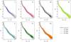 |
Fig. 6. HR diagrams for the seven populations, along with three PARSEC isochrones computed for AV = 0.15 and Z = 0.019. In all panels the light grey points show the entire sample. |
Cluster parameters from the literature.
The sequences of the different populations align with isochrones of different ages. We verified that sources fainter than MG = 5.5 and bluer than a log t = 7.5 isochrone in populations VI and VII are uniformly distributed across the investigated field of view. They therefore mostly correspond to contamination by main-sequence field stars and unresolved binaries. The remaining field star contamination in the older populations unfortunately overlaps too much with the PMS and cannot be easily identified on the basis of photometry.
We spatially divided the components of each population into several subgroups in order to estimate ages individually. For populations II, III, V, and VI, we manually split the population into two (eastern and western) subgroups. For population VI we selected the stars that lie within 1° of the centres of Collinder 135, Collinder 140, NGC 2451B, NGC 2547, and UBC 7 as their own subgroups. To split population VII (Vela OB2), we selected the stars that lie within 1° of the groups A, C, D, G, and H defined in Cantat-Gaudin et al. (2019). These divisions are marked on the maps of Appendix A.
We performed a maximum likelihood fitting of PARSEC isochrones through the observed MG and GBP − GRP for each population using a metallicity of Z = 0.019 and letting extinction and age be free parameters. The isochrones were reddened following the polynomial coefficients given in Gaia Collaboration (2018a). The resulting best-fit values are shown in Fig. 7. The procedure takes into account nominal photometric errors as well as the uncertainty on MG due to the parallax uncertainty. We remark that due to the millimagnitude quality of the photometry, the statistical uncertainty on the result is very small. We estimated the uncertainty on the best-fit age by making different samples of each subgroup, first based on the membership scores of Sect. 2.2 and then by bootstrapping redrawings. In all cases, the uncertainties on the best-fit age are below 0.05 in log t. This value does not reflect our actual uncertainty on the true age of the groups, which is dominated by the uncertainty on stellar evolution models and on the characterisation of the Gaia passbands. We find that using PARSEC isochrones computed with the passbands of Maíz Apellániz & Weiler (2018) increases all estimated log t by ∼0.05 and the passbands of Weiler (2018) by almost 0.1.
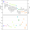 |
Fig. 7. Ages (top) and extinction AV (bottom) of the different subgroups, estimated from isochrone fitting. The error bar represents the statistical uncertainty and is smaller than the marker size for most groups. |
Although the interpretation of colour-magnitude diagrams for PMS stars and the presence of unresolved binaries can imitate age spreads (Hillenbrand et al. 2008; Baraffe et al. 2009), our simple fitting procedure highlights the fact that the different groups identified in this study are not coeval. The age derived here for the youngest groups of population VII are in agreement with the values of 7.5 ± 1 Myr derived by Jeffries et al. (2017) for the Vela OB2 association from optical photometry. The authors have shown, however, that lithium depletion patterns for these stars correspond to an older age (of 18–21 Myr) and that photometric ages of very young stars are likely underestimated. In any case, an age of ∼20 Myr would still make populatoin VII the youngest group in the sample investigated in this paper.
Because the reddening vector is mostly parallel to the pre-main sequence, extinction and age are not strongly degenerate. We remark, however, that the best-fit values of AV can be made lower when isochrones of higher metallicity are employed. This does not strongly affect the ages, in particular not the relative age distribution between the different subgroups.
The eastern groups of populations V and VI (both located farther away than 450 pc) exhibit a significantly higher extinction. This agrees with their position in the maps shown in Appendix D.
5. Comments on each population
5.1. Population I
This is the least populated and appears to be the oldest of the seven identified groups. It is also one of the most distant groups and occupies the north-east quarter of the investigated region in the distance range 450–550 pc (Fig. A.1).
Because its position correlates with the region of higher dust emission that is visible in Fig. 1, it is possible that this group is significantly affected by contamination from reddened zero-age main-sequence (ZAMS) stars. The location of this group in positional space and velocity space does correspond to an overdensity of blue stars (with GBP − GRP < 0.3), however, and the upper main-sequence stars of population I do not appear to be significantly redder than the rest of the sample.
Population I presents a very low contrast against field stars in spatial and astrometric space. Collecting additional information (for instance, additional radial velocities) might allow identifying more sources as associated with population I.
5.2. Population II
This group includes the known cluster Trumpler 10 and many stars that are mostly located in the northern half of the investigated region (b > −5°) at distances larger than 350 pc (Fig. A.2). The distribution appears continuous, with a high overdensity around the location of Trumpler 10 (∼420 pc) and a secondary overdensity in the north-west region (∼460 pc). Although this group is very elongated along the ℓ direction, its expansion rate (as modelled with a linear gradient) appears to be higher in the b direction (Fig. 5).
5.3. Population III
This group is mainly distributed in the southern half of the region (b < −5°) in two main subgroups (Fig. A.3). The eastern subgroup is denser and elongated. The western, sparser subgroup appears to occupy the cavity inside the ring-like structure reported by Cantat-Gaudin et al. (2019). Its projection also coincides with the structure known as the IRAS Vela Shell, and it could be the host population of the supernova that initiated the expansion of the shell.
5.4. Population IV
This group hosts the most stars. It stretches across the whole southern half of the region (Fig. A.4). It contains the known objects NGC 2547, NGC 2451B, Collinder 135, UBC 7, and Collinder 140. The dense clump that is visible in the top panel of Fig. A.4 about two degrees to the south of Collinder 135 is the object reported as UBC 7 by Castro-Ginard et al. (2018), for which the authors suggested a common origin with Collinder 135. The elongated structure that appears to bridge NGC 2547 to NGC 2451B is in fact located ∼100 pc closer than these two clusters. Its proper motions match the group identified as Cluster 6 by Beccari et al. (2018).
Population IV is especially interesting because its five densest clumps correspond to known clusters. Several authors have searched for pairs or multiple systems of open clusters (Piskunov et al. 2006; de la Fuente Marcos & de la Fuente Marcos 2009; Vázquez et al. 2010; Conrad et al. 2017) and proposed groupings based on statistical similarities between observed parameters. Soubiran et al. (2018) have proposed that Collinder 140 and NGC 2451B are related objects. In this study we show that NGC 2547, NGC 2451B, Collinder 135, UBC 7, and Collinder 140 not only share a common space motion, but are still physically connected by a continuous distribution of stars. We also show in Fig. B.1 that the cluster stars and the extended population overlap perfectly in a colour-absolute magnitude diagram and therefore show no appreciable age difference. The middle panel of Fig. A.4 shows that this population exhibits a significant level of kinematic substructure in addition to its radial expansion.
5.5. Population V
This group stretches along the southern border of the region (Fig. A.5) and shows two overdensities in the south-east and south-west corners. The eastern subgroup corresponds to group J from Cantat-Gaudin et al. (2019).
The western subgroup is older, sparser, and is not visible in the final density maps of Cantat-Gaudin et al. (2019) because the photometric selection and proper motion cuts applied in that study were designed to target the youngest known population (Vela OB2), while the slightly younger eastern subgroup is also more reddened. The two subgroups have slightly different vb velocities. The age and vb of the western subgroup are closer to the age and velocity of population IV, while the age and velocity of the eastern group are more similar to those of the younger groups.
Population V exhibits no significant expansion in the b (or Z direction). It appears to expand only along the direction of ℓ (see gradients in Fig. 5 and the middle panel of Fig. A.5).
5.6. Population VI
This group is made up of two main compact subgroups in the northern half of the region (Fig. A.6). The eastern subgroup is labelled I in Cantat-Gaudin et al. (2019), while the western subgroup is known as BH 23. Similarly to population V, this group exhibits a higher expansion rate in the direction of ℓ (or X) than in the vertical (b or Z) direction.
5.7. Population VII
This group is the second most populated after population IV. It is the densest, youngest, and most rapidly expanding group. Most of the stars identified by de Zeeuw et al. (1999) as members of the Vela OB2 association belong to this group.
Its spatial and kinematic substructure was studied in detail by Cantat-Gaudin et al. (2019), who remarked that its location and dimension correlate with the expanding structure known as the IRAS Vela Shell (IV; Sahu 1992; Sahu & Blaauw 1993). The authors suggested a common origin for these two objects in feedback from a supernova from an unidentified slightly older population. The newly discovered group labelled population III in this study is located inside the IVS and is ∼20 Myr older than population VII.
6. Discussion
The main result of this study is that a large portion of the stars in the Vela-Puppis region are not concentrated in the few previously known clusters, but are rather distributed in sparse structures that are elongated along the Galactic plane. They cluster in seven main groups in velocity space (top right panel of Fig. 3). We note a correlation between the age and position of these groups, and their location in (vℓ,vb) space. The youngest group (population VII) is located near (vℓ,vb) ≃ (0 km s−1,−20 km s−1). The two groups with vℓ > −20 km s−1 (populations V and VI) are located at low Galactic latitudes, while the others are located closer to the plane. This difference in velocity might be the result of a Galactic shear or the consequence of a velocity pattern that was already imprinted in the parent molecular cloud from which these young populations formed. We also note that the velocity vb seems to correlate with age, with the youngest group (population VII) having vb ∼ 0 km s−1, while the oldest groups (populations II and IV) reach vb ∼ −12 km s−1. We show that Collinder 135, Collinder 140, and the recently discovered UBC 7 are all part of population IV and are therefore related to the Vela complex, although they lie outside of the area studied by de Zeeuw et al. (1999), who defined the historical boundaries of the region that is referred to as the Vela OB2 association.
All seven groups show clear signs of (mostly non-isotropic) expansion; the youngest group expands most rapidly. A mechanism that is commonly invoked to explain the significant expansion rates of young clusters is residual gas expulsion (e.g. Hills 1980; Lada et al. 1984; Baumgardt & Kroupa 2007), where the gas that has not turned into stars (but still contributes to the total potential well of the stellar cluster) is dispersed by the feedback of the most massive young stars. This mechanism is expected to produce isotropic expansion profiles, however, and therefore cannot be the only mechanism responsible for the observed velocity structure of the populations characterised in this study.
Although we have shown beyond doubt that the overall spatial distribution of all identified populations is expanding, the Gaia DR2 we used is not sufficient to determine whether the denser clumps (the open clusters labelled in Fig. 1 as well as the dense subgroups of the youngest population) are bound, or are themselves slowly dispersing. Combining high-resolution spectroscopy and Gaia-DR1 astrometry, Bravi et al. (2018) have suggested that NGC 2547 might be in a supervirial state. A better characterisation could be obtained with Gaia DR2 data with a similar approach (see in e.g. Karnath et al. 2019, for Cep OB3). Interestingly, the observation that the distribution of young stars is more elongated along the ℓ direction than b has been made by Eggen (1980), who referred to the whole region as the “Vela sheet”. The boundaries of the volume we investigated here were chosen to exclude the extended spur of young stars from the Scorpius-Centaurus complex (see Fig. 1). We did not explore the possibility of a spatial or kinematical continuity between these two structures, although we note that the maps of Zari et al. (2018) report a lack of young stars that would form a bridge from Scorpius-Centaurus to Vela.
The portrait of the region drawn by this study is that of a highly substructured ensemble of young stars, with seven main kinematic groups whose formation is spread over ∼35 Myr. All of these groups physically extend over scales of several hundreds of parsecs. In agreement with Zari et al. (2018) (and at odds with Bouy & Alves 2015), we find no hint of a spatial gradient of age. This mixture of younger and older stars is indicative of multiple episodes of stellar formation over a short timescale. The chaotic aspect of the spatial distribution might reflect the turbulent structure of the primordial molecular cloud it formed from (e.g. Bonnell et al. 2003; Girichidis et al. 2011; Krumholz et al. 2012). The scale of the region as well as the velocity structure resemble the structures observed in numerical simulations of turbulent molecular clouds (e.g. Fujii 2015; Padoan et al. 2016, 2017). The age difference between the different populations is also similar to what is observed in supernovae-driven turbulent clouds (Padoan et al. in prep.). In this paradigm, the last episode of stellar formation (which formed population VII) would have been triggered by supernovae from the slightly older population II, which has the correct age and location for this scenario.
The volume of space investigated in this study is comparable with the dimensions of the nearby well-studied Scorpius–Centaurus (Sco-Cen) association. That region is composed of three main groups (Upper Scorpius, Upper Centaurus Lupus, and Lower Centaurus Crux Blaauw 1946; de Zeeuw et al. 1999; Wright & Mamajek 2018; Damiani 2018) with ages from ∼5 to ∼20 Myr (e.g. Pecaut & Mamajek 2016). It includes the two dense star-forming regions ρ Ophiucus and Lupus (hosting stars younger than ∼1 Myr). In order to explain that these two young groups are surrounded by older populations, Krause et al. (2018) recently proposed a “surround and squash” scenario in which the dispersed population forms first in a dense region of a large elongated molecular cloud. The feedback from its massive stars generates a superbubble of hot pressurised gas that eventually expands and surrounds the residual gas. It finally compresses this residual gas into pockets of young stars that are surrounded by a sparser and older population. This scenario also naturally allows the young subgroups to exhibit different velocities.
The Vela-Puppis region we investigated here presents similarities with Sco-Cen in terms of dimensions. It also features distinct groups of different ages, and its youngest group (population VII) is located at the centre. Vela-Puppis appears to be much more substructured spatially, however. Another difference is that all seven populations we identified show clear signs of expansion and formed as dense clusters (even the older ones), while Wright & Mamajek (2018) have shown that the three main older groups of Sco-Cen are not expanding. Because Vela-Puppis is older than Sco-Cen, it is possible that the previous generation of stars that produced the superbubble that squashed the current populations into existence have now dispersed and can no longer be identified in velocity or positional space. Population I from this study could be the youngest representant of this hypothetical dispersed generation, and Vela-Puppis would be an older, more substructured, and scaled-up version of Sco-Cen.
An argument against the “surround and squash” scenario being at play in Vela-Puppis is that the various groups observed here are not organised in pockets that are isolated from each other, but are instead rather extended and overlap partially. That one group of stars (belonging to population II) inside the ring formed by the younger population VII, which Cantat-Gaudin et al. (2019) have shown to match the projected location of the IRAS Vela Shell, is also an argument in favour of a more standard triggered star formation mechanism such as supernovae explosions or a “collect and collapse” (e.g. Elmegreen & Lada 1977; Zavagno et al. 2006; Dale et al. 2007; Elmegreen 2011) origin for population VII.
7. Conclusion
We used Gaia DR2 data to identify a large number of aggregates of young stars in a ∼600 square degree field in the direction of the Vela-Puppis constellations in the distance range 250–550 pc. We grouped them into seven main kinematic populations. From comparisons with theoretical isochrones, the apparent ages of these groups range from ∼8 to 50 Myr. The spatial structure of the groups extend across hundreds of parsecs, most of them with significant spatial and kinematic substructure. They all show clear signs of expansion along the Galactic X and Z axes (as determined from 3D velocities and from corrected tangential velocities), although this expansion is not isotropic for all groups, indicating that more than just internal mechanisms are at work. We observed no strong correlation between spatial location and age, but found correlations between kinematics (in particular velocity vb) and age, suggesting that star formation took place in a turbulent environment rather than following a monotonic spatial sequence.
The limited number of radial velocities in the Gaia-DR2 data as well as their relatively larger uncertainties prevent us from characterising the internal kinematics of the sub-components of the identified populations in greater detail. We therefore cannot determine whether the denser aggregates (the open clusters known prior to this study) are expanding or will remain gravitationally bound and remain clusters. Ground-based follow-up with high-resolution spectroscopy could provide precise radial velocity for a larger sample of stars and would also better constrain the stellar ages. This would help establish the time line for the stellar formation history of this complex region.
We recall that v ≃ 4.74 μ/ϖ, expressed in km s−1 if proper motion μ in mas yr−1 and parallax ϖ in mas.
Acknowledgments
We thank the anonymous referee for the helpful comments and constructive remarks that helped us to improve this manuscript. TCG thanks E. Zari for providing the map adapted in Fig. 1. TCG acknowledges support from Juan de la Cierva – formación 2015 grant, MINECO (FEDER/UE). This work was supported by the MINECO (Spanish Ministry of Economy) through grant ESP2016-80079-C2-1-R (MINECO/FEDER, UE) and MDM-2014-0369 of ICCUB (Unidad de Excelencia “María de Maeztu”). NJW acknowledges an STFC Ernest Rutherford Fellowship (grant number ST/M005569/1). PP acknowledges support by the Spanish MINECO under project AYA2017-88754-P. VMP acknowledges support by the Spanish MINECO under projects MDM-2014-0369 and AYA2017-88754-P. The preparation of this work has made extensive use of Topcat (Taylor 2005), and of NASA’s Astrophysics Data System Bibliographic Services, as well as the open-source Python packages Astropy (Astropy Collaboration 2013), numpy (Van Der Walt et al. 2011), and scikit-learn (Pedregosa et al. 2011). The figures in this paper were produced with Matplotlib (Hunter 2007). This research has made use of Aladin sky atlas developed at CDS, Strasbourg Observatory, France (Bonnarel et al. 2000; Boch & Fernique 2014). This work presents results from the European Space Agency (ESA) space mission Gaia. Gaia data are being processed by the Gaia Data Processing and Analysis Consortium (DPAC). Funding for the DPAC is provided by national institutions, in particular the institutions participating in the Gaia MultiLateral Agreement (MLA). The Gaia mission website is https://www.cosmos.esa.int/gaia. The Gaia archive website is https://archives.esac.esa.int/gaia.
References
- Ambartsumian, V. A. 1947, Stellar Evolution and Astrophysics (Yerevan: Armenian Acad. of Sci) [Google Scholar]
- Andrae, R., Fouesneau, M., Creevey, O., et al. 2018, A&A, 616, A8 [NASA ADS] [CrossRef] [EDP Sciences] [Google Scholar]
- Arenou, F., Luri, X., Babusiaux, C., et al. 2018, A&A, 616, A17 [Google Scholar]
- Armstrong, J. J., Wright, N. J., & Jeffries, R. D. 2018, MNRAS, 480, L121 [NASA ADS] [CrossRef] [Google Scholar]
- Astropy Collaboration (Robitaille, T. P., et al.) 2013, A&A, 558, A33 [NASA ADS] [CrossRef] [EDP Sciences] [Google Scholar]
- Bailer-Jones, C. A. L. 2015, PASP, 127, 994 [NASA ADS] [CrossRef] [Google Scholar]
- Baraffe, I., Chabrier, G., & Gallardo, J. 2009, ApJ, 702, L27 [NASA ADS] [CrossRef] [Google Scholar]
- Baumgardt, H., & Kroupa, P. 2007, MNRAS, 380, 1589 [NASA ADS] [CrossRef] [Google Scholar]
- Beccari, G., Boffin, H. M. J., Jerabkova, T., et al. 2018, MNRAS, 481, L11 [NASA ADS] [CrossRef] [Google Scholar]
- Blaauw, A. 1946, Publ. Kapteyn Astron. Lab. Gron., 52, 1 [NASA ADS] [Google Scholar]
- Blaauw, A. 1952, Bull. Astron. Inst. Neth., 11, 414 [NASA ADS] [Google Scholar]
- Blaauw, A. 1964, ARA&A, 2, 213 [NASA ADS] [CrossRef] [Google Scholar]
- Boch, T., & Fernique, P. 2014, in Astronomical Data Analysis Software and Systems XXIII, eds. N. Manset, & P. Forshay, ASP Conf. Ser., 485, 277 [NASA ADS] [Google Scholar]
- Bok, B. J. 1934, Harv. Coll. Obs. Circ., 384, 1 [NASA ADS] [Google Scholar]
- Bonnarel, F., Fernique, P., Bienaymé, O., et al. 2000, A&AS, 143, 33 [NASA ADS] [CrossRef] [EDP Sciences] [Google Scholar]
- Bonnell, I. A., Bate, M. R., & Vine, S. G. 2003, MNRAS, 343, 413 [NASA ADS] [CrossRef] [Google Scholar]
- Bossini, D., Vallenari, A., Bragaglia, A., et al. 2019, A&A, 623, A108 [NASA ADS] [CrossRef] [EDP Sciences] [Google Scholar]
- Bouy, H., & Alves, J. 2015, A&A, 584, A26 [NASA ADS] [CrossRef] [EDP Sciences] [Google Scholar]
- Bravi, L., Zari, E., Sacco, G. G., et al. 2018, A&A, 615, A37 [NASA ADS] [CrossRef] [EDP Sciences] [Google Scholar]
- Bressan, A., Marigo, P., Girardi, L., et al. 2012, MNRAS, 427, 127 [NASA ADS] [CrossRef] [Google Scholar]
- Briceño, C., Preibisch, T., Sherry, W. H., et al. 2007, Protostars and Planets V, 345 [Google Scholar]
- Brown, A. G. A., Dekker, G., & de Zeeuw, P. T. 1997, MNRAS, 285, 479 [NASA ADS] [CrossRef] [Google Scholar]
- Brown, A. G. A., Blaauw, A., Hoogerwerf, R., de Bruijne, J. H. J., & de Zeeuw, P. T. 1999, in NATO Advanced Science Institutes (ASI) Series C, eds. C. J. Lada, & N. D. Kylafis, 540, 411 [Google Scholar]
- Caballero, J. A., & Dinis, L. 2008, Astron. Nachr., 329, 801 [NASA ADS] [CrossRef] [Google Scholar]
- Cantat-Gaudin, T., Jordi, C., Vallenari, A., et al. 2018a, A&A, 618, A93 [NASA ADS] [CrossRef] [EDP Sciences] [Google Scholar]
- Cantat-Gaudin, T., Vallenari, A., Sordo, R., et al. 2018b, A&A, 615, A49 [NASA ADS] [CrossRef] [EDP Sciences] [Google Scholar]
- Cantat-Gaudin, T., Mapelli, M., Balaguer-Núñez, L., et al. 2019, A&A, 621, A115 [NASA ADS] [CrossRef] [EDP Sciences] [Google Scholar]
- Castro-Ginard, A., Jordi, C., Luri, X., et al. 2018, A&A, 618, A59 [NASA ADS] [CrossRef] [EDP Sciences] [Google Scholar]
- Comeron, F., Torra, J., & Gomez, A. E. 1998, A&A, 330, 975 [NASA ADS] [Google Scholar]
- Conrad, C., Scholz, R.-D., Kharchenko, N. V., et al. 2017, A&A, 600, A106 [NASA ADS] [CrossRef] [EDP Sciences] [Google Scholar]
- Dale, J. E., Bonnell, I. A., & Whitworth, A. P. 2007, MNRAS, 375, 1291 [NASA ADS] [CrossRef] [Google Scholar]
- Damiani, F. 2018, A&A, 615, A148 [NASA ADS] [CrossRef] [EDP Sciences] [Google Scholar]
- Damiani, F., Prisinzano, L., Jeffries, R. D., et al. 2017, A&A, 602, L1 [NASA ADS] [CrossRef] [EDP Sciences] [Google Scholar]
- de Bruijne, J. H. J. 1999, MNRAS, 306, 381 [NASA ADS] [CrossRef] [Google Scholar]
- de la Fuente Marcos, R., & de la Fuente Marcos, C. 2009, ApJ, 700, 436 [NASA ADS] [CrossRef] [Google Scholar]
- de Zeeuw, P. T., Hoogerwerf, R., de Bruijne, J. H. J., Brown, A. G. A., & Blaauw, A. 1999, AJ, 117, 354 [NASA ADS] [CrossRef] [Google Scholar]
- Dias, W. S., Alessi, B. S., Moitinho, A., & Lépine, J. R. D. 2002, A&A, 389, 871 [NASA ADS] [CrossRef] [EDP Sciences] [Google Scholar]
- Dravins, D., Lindegren, L., & Madsen, S. 1999, A&A, 348, 1040 [NASA ADS] [Google Scholar]
- Eddington, A. S. 1910, MNRAS, 71, 43 [NASA ADS] [CrossRef] [Google Scholar]
- Eggen, O. J. 1980, ApJ, 238, 627 [NASA ADS] [CrossRef] [Google Scholar]
- Elias, F., Cabrera-Caño, J., & Alfaro, E. J. 2006, AJ, 131, 2700 [NASA ADS] [CrossRef] [Google Scholar]
- Elmegreen, B. G. 2011, in EAS Pub. Ser., eds. C. Charbonnel, & T. Montmerle, 51, 31 [CrossRef] [Google Scholar]
- Elmegreen, B. G., & Lada, C. J. 1977, ApJ, 214, 725 [NASA ADS] [CrossRef] [Google Scholar]
- Ester, M., Kriegel, H. P., Sander, J., & Xu, X. 1996, Proceedings of the Second International Conference on Knowledge Discovery and Data Mining, KDD’96 (AAAI Press), 226 [Google Scholar]
- Evans, D. W., Riello, M., De Angeli, F., et al. 2018, A&A, 616, A4 [NASA ADS] [CrossRef] [EDP Sciences] [Google Scholar]
- Franciosini, E., Sacco, G. G., Jeffries, R. D., et al. 2018, A&A, 616, L12 [NASA ADS] [CrossRef] [EDP Sciences] [Google Scholar]
- Fujii, M. S. 2015, PASJ, 67, 59 [NASA ADS] [CrossRef] [Google Scholar]
- Gaia Collaboration (Brown, A. G. A., et al.) 2016a, A&A, 595, A2 [NASA ADS] [CrossRef] [EDP Sciences] [Google Scholar]
- Gaia Collaboration (Prusti, T., et al.) 2016b, A&A, 595, A1 [NASA ADS] [CrossRef] [EDP Sciences] [Google Scholar]
- Gaia Collaboration (Babusiaux, C., et al.) 2018a, A&A, 616, A10 [NASA ADS] [CrossRef] [EDP Sciences] [Google Scholar]
- Gaia Collaboration (Brown, A. G. A., et al.) 2018b, A&A, 616, A1 [NASA ADS] [CrossRef] [EDP Sciences] [Google Scholar]
- Gilmore, G., Randich, S., Asplund, M., et al. 2012, The Messenger, 147, 25 [NASA ADS] [Google Scholar]
- Girichidis, P., Federrath, C., Banerjee, R., & Klessen, R. S. 2011, MNRAS, 413, 2741 [NASA ADS] [CrossRef] [Google Scholar]
- Hillenbrand, L. A., Bauermeister, A., & White, R. J. 2008, in 14th Cambridge Workshop on Cool Stars, Stellar Systems, and the Sun, ed. G. van Belle, ASP Conf. Ser., 384, 200 [NASA ADS] [Google Scholar]
- Hills, J. G. 1980, ApJ, 235, 986 [NASA ADS] [CrossRef] [Google Scholar]
- Hoogerwerf, R., & Aguilar, L. A. 1999, MNRAS, 306, 394 [NASA ADS] [CrossRef] [Google Scholar]
- Hunter, J. D. 2007, Comput. Sci. Eng., 9, 90 [NASA ADS] [CrossRef] [Google Scholar]
- Jeffries, R. D., Naylor, T., Walter, F. M., Pozzo, M. P., & Devey, C. R. 2009, MNRAS, 393, 538 [NASA ADS] [CrossRef] [Google Scholar]
- Jeffries, R. D., Jackson, R. J., Cottaar, M., et al. 2014, A&A, 563, A94 [NASA ADS] [CrossRef] [EDP Sciences] [Google Scholar]
- Jeffries, R. D., Jackson, R. J., Franciosini, E., et al. 2017, MNRAS, 464, 1456 [NASA ADS] [CrossRef] [Google Scholar]
- Jones, D. H. P. 1971, MNRAS, 152, 231 [NASA ADS] [CrossRef] [Google Scholar]
- Kaltcheva, N. T., & Hilditch, R. W. 2000, MNRAS, 312, 753 [NASA ADS] [CrossRef] [Google Scholar]
- Kapteyn, J. C. 1914, ApJ, 40, 43 [NASA ADS] [CrossRef] [Google Scholar]
- Karnath, N., Prchlik, J. J., Gutermuth, R. A., et al. 2019, ApJ, 871, 46 [NASA ADS] [CrossRef] [Google Scholar]
- Kharchenko, N. V., Piskunov, A. E., Schilbach, E., Röser, S., & Scholz, R.-D. 2013, A&A, 558, A53 [NASA ADS] [CrossRef] [EDP Sciences] [Google Scholar]
- Kos, J., Bland-Hawthorn, J., Asplund, M., et al. 2018, A&A, submitted [arXiv:1811.11762] [Google Scholar]
- Kounkel, M., Covey, K., Suárez, G., et al. 2018, AJ, 156, 84 [NASA ADS] [CrossRef] [Google Scholar]
- Krause, M. G. H., Burkert, A., Diehl, R., et al. 2018, A&A, 619, A120 [NASA ADS] [CrossRef] [EDP Sciences] [Google Scholar]
- Krone-Martins, A., & Moitinho, A. 2014, A&A, 561, A57 [NASA ADS] [CrossRef] [EDP Sciences] [Google Scholar]
- Krumholz, M. R., Klein, R. I., & McKee, C. F. 2012, ApJ, 754, 71 [NASA ADS] [CrossRef] [Google Scholar]
- Kuhn, M. A., Hillenbrand, L. A., Sills, A., Feigelson, E. D., & Getman, K. V. 2019, ApJ, 870, 32 [Google Scholar]
- Lada, C. J., Margulis, M., & Dearborn, D. 1984, ApJ, 285, 141 [NASA ADS] [CrossRef] [Google Scholar]
- Lesh, J. R. 1968, ApJ, 152, 905 [NASA ADS] [CrossRef] [Google Scholar]
- Lindegren, L. 2018, Gaia Technical Note, GAIA-C3-TN-LU-LL-124-0 [Google Scholar]
- Lindegren, L., Hernández, J., Bombrun, A., et al. 2018, A&A, 616, A2 [NASA ADS] [CrossRef] [EDP Sciences] [Google Scholar]
- Luri, X., Brown, A. G. A., Sarro, L. M., et al. 2018, A&A, 616, A9 [NASA ADS] [CrossRef] [EDP Sciences] [Google Scholar]
- Maíz Apellániz, J., & Weiler, M. 2018, A&A, 619, A180 [NASA ADS] [CrossRef] [EDP Sciences] [Google Scholar]
- Mapelli, M., Vallenari, A., Jeffries, R. D., et al. 2015, A&A, 578, A35 [NASA ADS] [CrossRef] [EDP Sciences] [Google Scholar]
- Mineur, H. 1939, Ann. Astrophys., 2, 1 [NASA ADS] [Google Scholar]
- Miville-Deschênes, M.-A., & Lagache, G. 2005, ApJS, 157, 302 [NASA ADS] [CrossRef] [Google Scholar]
- Müllner, D. 2011, ArXiv e-prints [arXiv:1109.2378] [Google Scholar]
- Padoan, P., Pan, L., Haugbølle, T., & Nordlund, Å. 2016, ApJ, 822, 11 [NASA ADS] [CrossRef] [Google Scholar]
- Padoan, P., Haugbølle, T., Nordlund, Å., & Frimann, S. 2017, ApJ, 840, 48 [NASA ADS] [CrossRef] [Google Scholar]
- Pecaut, M. J., & Mamajek, E. E. 2016, MNRAS, 461, 794 [NASA ADS] [CrossRef] [Google Scholar]
- Pedregosa, F., Varoquaux, G., Gramfort, A., et al. 2011, J. Mach. Learn. Res., 12, 2825 [Google Scholar]
- Piskunov, A. E., Kharchenko, N. V., Röser, S., Schilbach, E., & Scholz, R.-D. 2006, A&A, 445, 545 [NASA ADS] [CrossRef] [EDP Sciences] [Google Scholar]
- Pozzo, M., Jeffries, R. D., Naylor, T., et al. 2000, MNRAS, 313, L23 [NASA ADS] [CrossRef] [Google Scholar]
- Randich, S., Gilmore, G., & Gaia-ESO Consortium 2013, The Messenger, 154, 47 [NASA ADS] [Google Scholar]
- Rasmuson, N. H. 1921, Meddelanden fran Lunds Astronomiska Observatorium Serie, II, 3 [NASA ADS] [Google Scholar]
- Sacco, G. G., Jeffries, R. D., Randich, S., et al. 2015, A&A, 574, L7 [NASA ADS] [CrossRef] [EDP Sciences] [Google Scholar]
- Sahu, M. S. 1992, PhD thesis, Kapteyn Institute, The Netherlands [Google Scholar]
- Sahu, M., & Blaauw, A. 1993, in Massive Stars: Their Lives in the Interstellar Medium, eds. J. P. Cassinelli, & E. B. Churchwell, ASP Conf. Ser., 35, 278 [NASA ADS] [Google Scholar]
- Sanders, J. L., & Das, P. 2018, MNRAS, 481, 4093 [NASA ADS] [CrossRef] [Google Scholar]
- Soubiran, C., Cantat-Gaudin, T., Romero-Gomez, M., et al. 2018, A&A, 619, A155 [NASA ADS] [CrossRef] [EDP Sciences] [Google Scholar]
- Taylor, M. B. 2005, in Astronomical Data Analysis Software and Systems XIV, eds. P. Shopbell, M. Britton, & R. Ebert, ASP Conf. Ser., 347, 29 [Google Scholar]
- Van Der Walt, S., Colbert, S. C., & Varoquaux, G. 2011, Comput. Sci. Eng., 13, 22 [CrossRef] [Google Scholar]
- Vasiliev, E. 2018, MNRAS, submitted [arXiv:1811.05345] [Google Scholar]
- Vázquez, R. A., Moitinho, A., Carraro, G., & Dias, W. S. 2010, A&A, 511, A38 [NASA ADS] [CrossRef] [EDP Sciences] [Google Scholar]
- Weiler, M. 2018, A&A, 617, A138 [NASA ADS] [CrossRef] [EDP Sciences] [Google Scholar]
- Wright, N. J., & Mamajek, E. E. 2018, MNRAS, 476, 381 [NASA ADS] [CrossRef] [Google Scholar]
- Zari, E., Hashemi, H., Brown, A. G. A., Jardine, K., & de Zeeuw, P. T. 2018, A&A, 620, A172 [NASA ADS] [CrossRef] [EDP Sciences] [Google Scholar]
- Zavagno, A., Deharveng, L., Comerón, F., et al. 2006, A&A, 446, 171 [NASA ADS] [CrossRef] [EDP Sciences] [Google Scholar]
Appendix A: Maps
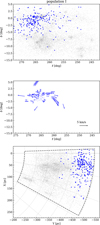 |
Fig. A.1. Top: location of the population I stars on the sky. Middle: vectors represent the local mean tangential velocity in a 0.5° radius (with respect to the group median) if at least three stars are present. The velocities are corrected for virtual contraction through the mean radial velocity of the population. Bottom: location of the same stars projected on the Galactic plane. |
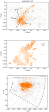 |
Fig. A.7. Same as Fig. A.1 for population VII. The subgroups are labelled as in Cantat-Gaudin et al. (2019). |
Appendix B: Extended component of population IV
The extended distribution of stars around the known open clusters (NGC 2547, NGC 2451B, Collinder 135, UBC 7, and Collinder 140) of population IV might be interpreted at first glance as field contamination. In Fig. B.1 we compare the photometry (in a colour-absolute magnitude diagram) of stars in three density groups: the high-density clusters, the surrounding extended population, and the low-density outskirts.
The extended intermediate-density group perfectly overlaps with the known clusters, suggesting that these stars have the same age and are related to the clusters. The stars in the low-density outskirts, however, exhibit discrepant photometry and can therefore be considered as unrelated field stars that coincidentally share the same velocity as population IV stars. An a priori photometric selection of members is more difficult for population IV than for populations VI and VII, however, because of its older age (and therefore the proximity of the main-sequence field stars to the PMS stars in photometric space).
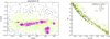 |
Fig. B.1. Left: members of population IV (same as top panel of Fig. A.4), colour-coded by local density (number of neighbours within one degree). Right: colour–absolute magnitude diagram using the same colour code. |
Appendix C: Correcting for virtual contraction
The bulk motion of a group of stars moving away from us introduces a perspective effect that causes an apparent contraction of their spatial distribution, where the proper motion or tangential velocity vectors (when plotted with respect to the mean of the group) point inwards. This also results in a negative gradient of velocity vℓ with respect to Galactic longitude ℓ (and similarly, vb with respect to b). The top panel of Fig. C.1 shows that such apparent velocity gradients are visible in most of the identified populations.
The expected virtual motion of each star can be calculated as a function of the assumed bulk velocity of the group and the position of the star from the centre of the group. The equations we used in this study are those of Brown et al. (1997) and are recalled in Sect. 3.2.
In Fig. C.1 we show that for population II, the observed tangential velocity trend with ℓ is not as steep as expected from its mean radial velocity. In order to match the observed slope, we need to assume a radial velocity of 13 km s−1, which is largely beyond the uncertainty range (23±0.4 km s−1). The positive gradient in the residuals (bottom panel of Fig. C.1) is indicative of expansion along the Galactic plane.
We list in Table 1 the residual slopes observed after correction in the seven identified populations. The middle panels of Figs. A.1–A.7 show that all of them exhibit significant expansion. The expansion rate of population VII is the highest and is stronger than its virtual contraction (Cantat-Gaudin et al. 2019).
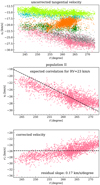 |
Fig. C.1. Top: observed tangential velocity vℓ as a function of Galactic longitude for populations II to VII. Middle: same as top panel, showing only population II. The dashed line is the expected relation for a non-expanding group of stars with systemic velocity 23 km s−1 (shifted vertically to overlap with the observed data). Bottom: corrected velocity (residuals of the observed velocities minus virtual contraction correction). |
Appendix D: Extinction map
In this section we use the values of extinction AG provided in the Gaia DR2 catalogue (Andrae et al. 2018) to map the extinction in difference distances ranges, from 0 to 1 kpc. To perform this experiment, we used all stars available in this volume of space and employed no photometric selection. The result is shown in Fig. D.1. Although the individual values are noisy (with large uncertainties for individual stars) and overestimated for AG lower than ∼0.5 (Andrae et al. 2018; Sanders & Das 2018), these data are sufficient to show that stars within 350 pc are virtually unaffected by interstellar extinction, and that stars with b > −5° are unaffected out to ∼500 pc.
The few pixels of relatively higher extinction near (ℓ,b) = (263,−7.5) in the bottom panel of Fig. D.1 correspond to the Gamma Velorum cluster, whose young PMS stars are interpreted as reddened main-sequence stars by the procedure of Andrae et al. (2018).
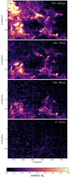 |
Fig. D.1. Median value of extinction (AG) from the Gaia DR2 catalogue for stars in four different distance ranges. |
All Tables
All Figures
|
Fig. 1. Left: composite of an IRIS 60 μm image (Miville-Deschênes & Lagache 2005) and DSS optical image of the investigated region. Right: distribution of PMS stars projected on the Galactic plane from Zari et al. (2018). The radii of the concentric circles centred on the Sun increase from 100 to 500 pc. |
| In the text | |
|
Fig. 2. Photometric selection of young stars. The reference stars are the members of the young clusters Trumpler 10, NGC 2451B, NGC 2547, Collinder 135, Collinder 140, and the Gamma Velorum cluster (Pozzo 1). The dashed line corresponds to the zero-age main sequence for a PARSEC isochrone of metallicity Z = 0.019 and AV = 0.15. |
| In the text | |
|
Fig. 3. Top left: proper motions of the stars with UPMASK clustering scores larger than 50%. Top right: tangential velocities (in Galactic coordinates) of the same stars. The colours correspond to the seven populations defined from their tangential velocities (see text). Bottom: spatial distribution of the same stars. |
| In the text | |
|
Fig. 4. Gaia DR2 radial velocity as a function of distance for the stars in each population identified in this study. κr: slope of the radial velocity gradient with distance (×10−2 km s−1 pc−1). μ: mean radial velocity (km s−1). σ: standard deviation (km s−1). σ/ |
| In the text | |
|
Fig. 5. Observed linear expansion rates (as listed in Table 1). Squares: (κX,κZ) from 3D velocities. Dots: (κℓ,κb) from corrected tangential velocities (see Sect. 3.2). The colour-coding is the same as in Figs. 3 and 4. |
| In the text | |
|
Fig. 6. HR diagrams for the seven populations, along with three PARSEC isochrones computed for AV = 0.15 and Z = 0.019. In all panels the light grey points show the entire sample. |
| In the text | |
|
Fig. 7. Ages (top) and extinction AV (bottom) of the different subgroups, estimated from isochrone fitting. The error bar represents the statistical uncertainty and is smaller than the marker size for most groups. |
| In the text | |
|
Fig. A.1. Top: location of the population I stars on the sky. Middle: vectors represent the local mean tangential velocity in a 0.5° radius (with respect to the group median) if at least three stars are present. The velocities are corrected for virtual contraction through the mean radial velocity of the population. Bottom: location of the same stars projected on the Galactic plane. |
| In the text | |
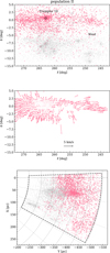 |
Fig. A.2. Same as Fig. A.1 for population II. |
| In the text | |
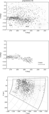 |
Fig. A.3. Same as Fig. A.1 for population III. |
| In the text | |
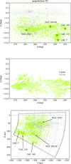 |
Fig. A.4. Same as Fig. A.1 for population IV. |
| In the text | |
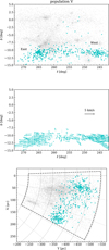 |
Fig. A.5. Same as Fig. A.1 for population V. |
| In the text | |
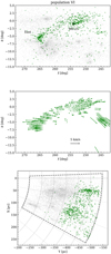 |
Fig. A.6. Same as Fig. A.1 for population VI. |
| In the text | |
|
Fig. A.7. Same as Fig. A.1 for population VII. The subgroups are labelled as in Cantat-Gaudin et al. (2019). |
| In the text | |
|
Fig. B.1. Left: members of population IV (same as top panel of Fig. A.4), colour-coded by local density (number of neighbours within one degree). Right: colour–absolute magnitude diagram using the same colour code. |
| In the text | |
|
Fig. C.1. Top: observed tangential velocity vℓ as a function of Galactic longitude for populations II to VII. Middle: same as top panel, showing only population II. The dashed line is the expected relation for a non-expanding group of stars with systemic velocity 23 km s−1 (shifted vertically to overlap with the observed data). Bottom: corrected velocity (residuals of the observed velocities minus virtual contraction correction). |
| In the text | |
|
Fig. D.1. Median value of extinction (AG) from the Gaia DR2 catalogue for stars in four different distance ranges. |
| In the text | |
Current usage metrics show cumulative count of Article Views (full-text article views including HTML views, PDF and ePub downloads, according to the available data) and Abstracts Views on Vision4Press platform.
Data correspond to usage on the plateform after 2015. The current usage metrics is available 48-96 hours after online publication and is updated daily on week days.
Initial download of the metrics may take a while.