| Issue |
A&A
Volume 625, May 2019
|
|
|---|---|---|
| Article Number | A39 | |
| Number of page(s) | 9 | |
| Section | Stellar atmospheres | |
| DOI | https://doi.org/10.1051/0004-6361/201935352 | |
| Published online | 07 May 2019 | |
High-precision analysis of binary stars with planets
I. Searching for condensation temperature trends in the HD 106515 system★
1
Instituto de Ciencias Astronómicas, de la Tierra y del Espacio (ICATE-CONICET),
C.C 467,
5400 San Juan, Argentina
e-mail: This email address is being protected from spambots. You need JavaScript enabled to view it.
2
Facultad de Ciencias Exactas, Universidad Nacional de San Juan (UNSJ), Físicas y Naturales (FCEFN), San Juan, Argentina
3
Observatorio Astronómico de Córdoba (OAC),
Laprida 854,
X5000BGR
Córdoba, Argentina
4
Departamento de Física y Astronomía, Universidad de La Serena,
Av. Cisternas 1200. 1720236
La Serena, Chile
5
Consejo Nacional de Investigaciones Científicas y Técnicas (CONICET), Argentina
6
Instituto de Astronomía, Universidad Nacional Autónoma de México, Ciudad Universitaria, Ciudad de México
04510, México
Received:
24
February
2019
Accepted:
1
April
2019
Abstract
Aims. We explore for the first time the probable chemical signature of planet formation in the remarkable binary system HD 106515. Star A hosts a massive long-period planet with ~9 MJup detected by radial velocity, while there is no planet detected at the B star. We also refine stellar and planetary parameters by using non-solar-scaled opacities when modelling the stars.
Methods. We carried out a simultaneous determination of stellar parameters and abundances by applying for the first time non-solar-scaled opacities in this binary system, in order to reach the highest possible precision. We used a line-by-line strictly differential approach, using the Sun and then the A star as reference. Stellar parameters were determined by imposing an ionization and excitation balance of Fe lines, with an updated version of the FUNDPAR program, ATLAS12 model atmospheres, and the MOOG code. Opacities for an arbitrary composition were calculated through the opacity sampling method. The chemical patterns were compared with solar-twins condensation temperature Tc trends from the literature and also mutually between both stars. We take the opportunity to compare and discuss the results of the classical solar-scaled method and the high-precision procedure applied here.
Results. Stars A and B in the binary system HD 106515 do not seem to be depleted in refractory elements, which is different when comparing the Sun with solar twins. The terrestrial planet formation would have been less efficient in the stars of this binary system. Together with HD 80606/7, this is the second binary system that does not seem to present a (terrestrial) signature of planet formation, when both systems host an eccentric giant planet. This is in agreement with numerical simulations, where the early dynamical evolution of eccentric giant planets clears out most of the possible terrestrial planets in the inner zone. We refined the stellar mass, radius, and age for both stars and found a notable difference of ~78% in R⋆ compared to previous works. We also refined the planet mass to mp sini = 9.08 ± 0.20 MJup, which differs by ~6% compared with the literature. In addition, we showed that the non-solar-scaled solution is not compatible with the classical solar-scaled method, and some abundance differences are comparable to non-local thermodynamic equilibrium (NLTE) or galactic chemical evolution (GCE) effects especially when using the Sun as reference. Therefore, we encourage the use of non-solar-scaled opacities in high-precision studies such as the detection of Tc trends.
Key words: stars: abundances / planetary systems / binaries: visual / stars: individual: HD 106515
The data presented herein were obtained at the W.M. Keck Observatory, which is operated as a scientific partnership between the California Institute of Technology, the University of California, and the National Aeronautics and Space Administration. The Observatory was made possible by the generous financial support of the W.M. Keck Foundation.
© ESO 2019
1 Introduction
In recent years, the achieved high precision in the derivation of stellar parameters and chemical abundances has allowed us to study in detail possible differences in stars with and without planets (e.g. Meléndez et al. 2009; Ramírez et al. 2011; Bedell et al. 2014; Saffe et al. 2017). For instance, the search for planet formation or accretion signatures in the photospheric composition of the stars was performed by looking at the condensation temperature Tc trends, with an unprecedented dispersion in metallicity below ~0.01 dex (e.g. Meléndez et al. 2009; Liu et al. 2014; Saffe et al. 2015, 2016, 2017). In particular, Meléndez et al. (2009; hereafter M09) detected a deficiency in refractory elements in the Sun with respect to 11 solar twins, suggesting that the refractory elements depleted in the solar photosphere are possibly trapped in terrestrial planets and/or in the cores of giant planets. The same conclusion was also reached by Ramírez et al. (2009, 2010), using larger samples of solar twins and analogues.
The study of binary or multiple systems plays a central role in the detection of the possible chemical signature of planet formation, providing that the stars were born from the same molecular cloud. Differential abundances between the components of these systems greatly diminishes effects such as galactic chemical evolution (GCE) or the galactic birth place of the stars, which could affect Tc trends (see e.g. González Hernández et al. 2013; Adibekyan et al. 2014, 2016). In addition, the analysis of two physically similar starsusing one of them as a reference star allows us to diminish the dispersion in both the derivation of stellar parameters and chemical abundances (e.g. Saffe et al. 2015). Therefore, a binary system with similar stellar components where only one of them is orbited by a planet is an ideal laboratory to look for very small chemical differences that could be attributed to the planet formation process.
To date, although more than ~2990 planetary systems are known1, to find thesekind of systems has proven to be a very difficult task. Examples of these binary systems previously studied in the literature include 16 Cyg, HAT-P-1, HD 80606, and HAT-P-4 (e.g. Ramírez et al. 2011; Liu et al. 2014; Saffe et al. 2015, 2017). There are also binary systems in which circumstellar planets orbit both stars of the system, such as HD 20781, HD 133131, and WASP-94 (Mack et al. 2014; Teske et al. 2016a,b). Then, there is a need for additional stars hosting planets in binary systems to be compared through a high-precision abundance determination. Due to their importance, some of these unique systems such as 16 Cyg received the attention of many different works studying their chemical composition in detail (e.g. Laws & Gonzalez 2016; Takeda 2005; Schuler et al. 2011; Ramírez et al. 2011; Tucci Maia et al. 2014). Some works suggested that both stars present the same chemical composition (Takeda 2005; Schuler et al. 2011)while other studies found that 16 Cyg A is more metal rich than the planet host B component (Laws & Gonzalez 2016; Ramírez et al. 2011; Tucci Maia et al. 2014; Nissen et al. 2017). In addition, the complete Tc trend detected by Tucci Maia et al. (2014) between the stars of 16 Cyg covers a range of only 0.04 dex between the maximum and minimum abundance values of 19 different chemical species (see their Fig. 3). More recently, Nissen et al. (2017) performed a high-precision analysis of this pair using High Accuracy Radial velocity Planet Searcher for the Northern hemisphere (HARPS-N) spectra and found a clear trend with Tc. These examples show that the detection of a chemical difference or a possible Tc trend as a chemical signature of planet formation is a challenge, and does require the maximum precision in both stellar parameters and abundances (for a more complete discussion, see also Saffe et al. 2018). Recently, our group achieved a major step forward in the pursuit of the highest possible precision. For the first time, we used non-solar-scaled opacities in a simultaneous derivation of both stellar parameters and abundances (Saffe et al. 2018) for main sequence and giant stars. When modelling the atmosphere of the stars, the four stellar parameters usually taken as Teff, log g, [Fe/H], and vmicro are now taken as Teff, log g, chemical pattern, and vmicro. In this way, we showed that many chemical species show a small but noticeable variation when using the new doubly iterated method instead of the usual solar-scaled methods, implying that Tc trends could also vary. We started a new programme in order to detect the possible chemical signature of planet formation in these binary systems by taking advantage of this improvement in the technique.
Mayor et al. (2011) first announced through a preprint the detection of a high-mass giant planet orbiting the star HD 106515 A with a period of ~9.9 yr and a minimum mass m sin i ~ 10 MJup, as a part of a HARPS radial velocity (RV) survey. The true mass of this object could correspond to the transition region between planets and brown dwarfs. The host star belongs to a wide binary system together with HD 106515 B, separated by 7.5 arcsec (~250 AU), in which both stars have a similar mass and a metallicity close to solar (Desidera et al. 2004, 2006). The presence of this massive planet was later confirmed in the work of Desidera et al. (2012), who performed a RV monitoring of both stars in this system using Spettrografo Alta Risoluzione Galileo (SARG) spectra. However, the authors do not find significant RV variations on the B star, and rule out additional stellar companions by using adaptive optics images. They propose that the relatively high eccentricity of the planet (0.572 ± 0.011) may arise from the Kozai mechanism, that is, a dynamical perturbation due to the presence of the wide stellar component. Marmier et al. (2013) updated some orbital parameters of the planet by using CORALIE2 spectra, and proposed a possible Kozai mechanism similar to Desidera et al. (2012). We note that this binary system is remarkable for a number of reasons. First, there is a notable similarity between the stars of thissystem, which show an estimated difference in effective temperature and superficial gravity of +157 ± 11 K and −0.02 ± 0.15 dex (Desidera et al. 2004), taken as A − B. This makes HD 106515 a unique target to analyse through a differential study, belonging to the select group of binary systems with similar components and having a planet orbiting only one star. Second, from more than ~2990 planetary systems detected, only 28 of them (<0.1%) are known with a period greater than 9 yr. The long period coverage is very important in order to properly constrain models of planet formation and migration. In addition, with a mass higher than 6 MJup, this planet belong to the upper ~15% of the planetary mass distribution (see e.g. Marmier et al. 2013). Therefore, the study of this object give us the possibility, for the first time, to test the possible chemical signature of planet formation for the case of a high-mass long-period planet. We take advantage of our recent improvement in the derivation of high-precision abundances (Saffe et al. 2018) to study this notable binary system with a line-by-line differential approach, aiming to detect a slight contrast between the components.
This work is organized as follows. In Sect. 2 we describe the observations and data reduction, while in Sect. 3 we present the stellar parameters and chemical abundance analysis, and present a refined value for the planetary mass. In Sect. 4 we show the results and discussion, and finally in Sect. 5 we highlight our main conclusions.
2 Observations and data reduction
Observations of the HD 106515 binary system were acquired using the High Resolution Echelle Spectrometer (HIRES, Vogt et al. 1994) attached to the right Nasmyth platform of the Keck 10-m telescope on Mauna Kea, Hawaii. HIRES is a grating cross-dispersed echelle spectrograph, equipped with a 2048 × 4096 Massachusets Institute of Technology-Lincoln Laboratory (MIT-LL) detector with a pixel size of 15 μm. The stellar spectra for this work were downloaded from the Keck Observatory Archive (KOA)3, under the program ID N158Hr. The slit used was B2 with a width of 0.574 arcsec, which provides a measured resolution of ~67 000 at ~5200 Å4.
The observations were taken on December 9, 2013, with the B star observed immediately after the A star, using the same spectrograph configuration for both objects. The exposure times were 180 and 240 s on each target, obtaining a final signal-to-noise ratio (S/N) of ~300 measured at ~6000 Å. The final spectral coverage is ~4700–8900 Å. The asteroid Iris was also observed with the same spectrograph set-up, achieving a similar S/N, to acquire the solar spectrum useful for reference in our (initial) differential analysis. We note, however, that the final differential study with the highest abundance precision is between stars A and B because of their high degree of similarity.
HIRES spectra were reduced using the data reduction package MAKEE5 (MAuna Kea Echelle Extraction), which performs the usual reduction process including bias subtraction, flat fielding, spectral order extractions, and wavelength calibration. The continuum normalization and other operations (such as Doppler correction) were performed using Image Reduction and Analysis Facility (IRAF)6.
3 Stellar parameters and chemical abundance analysis
We derived the fundamental parameters (Teff, log g, chemical pattern, vmicro) of stars A and B following the same procedure detailed in our previous work (Saffe et al. 2018). We started by measuring the equivalent widths (EW) of Fe I and Fe II lines in the spectra of our programme stars using the IRAF task splot, and then continued with other chemical species. The lines list and relevant laboratory data were taken from Liu et al. (2014), Meléndez et al. (2014), and then extended with data from Bedell et al. (2014), who carefully selected lines for a high-precision abundance determination.
Stellar parameters and abundances were derived simultaneously by imposing excitation and ionization balance of Fe I and Fe II lines. We used an updated version of the program FUNdamental PARameters (FUNDPAR, Saffe 2011; Saffe et al. 2018), which uses the MOOG code (Sneden 2016) together with ATLAS12 model atmospheres (Kurucz 1993) to search for the appropriate solution. The procedure uses explicitly calculated (i.e. non-interpolated) plane-parallel local thermodynamic equilibrium (LTE) Kurucz’s model atmospheres, including the internal calculation of specific opacities through the opacity sampling (OS) method. The first FUNDPAR iterative process searches the iron balance with the usual solar-scaled model atmospheres. A starting set of parameters and abundances is determined using EWs and spectral synthesis. Then, the iterativeprocess in FUNDPAR is restarted, but using ATLAS12 model atmospheres scaled to the last set of abundances found. This new iteration includes the calculation of specific opacities for the last chemical pattern specified, and not only a mere change in the abundances of the model. Thus, ATLAS12 models are described as (Teff, log g, chemical pattern, vmicro) rather than the usual solar-scaled (Teff, log g, [Fe/H], vmicro). New stellar parameters and abundances are then successively derived, finishing the process consistently when the stellar parameters are the same as the previous step (for more details, see Saffe et al. 2018).
Stellar parameters of stars A and B were determined by applying the full7 line-by-line differential technique, using the Sun as standard in an initial approach, and then we recalculated the parameters of the B star using A as reference. Firstly, we derived absolute abundances for the Sun using 5777 K for Teff, 4.44 dex for log g and an initial vturb of 1.0 km s−1. Then, the solar vturb was estimated by requiring zero slope in the absolute abundances of Fe I lines versus EWr and obtained a final vturb of 0.91 km s−1. We note, however, that the exact values are not crucial for our strictly differential study (see e.g. Bedell et al. 2014; Saffe et al. 2015).
The next step was the determination of stellar parameters of stars A and B using the Sun as standard, that is, (A − Sun) and (B − Sun). The resulting stellar parameters for star A were Teff = 5364 ± 57 K, log g = 4.39 ± 0.18 dex, [Fe/H] = +0.016 ± 0.009 dex, and vturb = 0.79 ± 0.12 km s−1. For star B we obtained Teff = 5190 ± 58 K, log g = 4.30 ± 0.20 dex, [Fe/H] = +0.022 ± 0.010 dex, and vturb = 0.58 ± 0.15 km s−1. The errors in the stellar parameters were derived following the procedure detailed in Saffe et al. (2015), which takes into account the individual and the mutual covariance terms of the error propagation. We present in Figs. 1and 2 abundance versus excitation potential and abundance versus reduced equivalent width (EWr) for both stars. Filled and empty points correspond to Fe I and Fe II, while the dashed lines are linear fits to the differential abundance values.
The stellar parameters and abundances of the B star were then redetermined, but using the A star as reference instead of the Sun (B − A) to perform the differential analysis. Similar to previous works, we chose the hotter star of the pair as reference (e.g. Saffe et al. 2015, 2016, 2017). Figure 3 shows the plots of abundance versus excitation potential and abundance versus EWr, using similar symbols to those used in Figs. 1 and 2. The resulting stellar parameters for star B are the same as those obtained when we used the Sun as a reference, Teff = 5190 ± 48 K, log g = 4.30 ± 0.17 dex, [Fe/H] = +0.022 ± 0.009 dex, and vturb = 0.58 ± 0.12 km s−1.
We computed the individual abundances for the following elements: C I, O I, Na I, Mg I, Al I, Si I, S I, Ca I, Sc I, Sc II, Ti I, Ti II, V I, Cr I, Cr II, Mn I, Fe I, Fe II, Co I, Ni I, Cu I, Sr I, Y II, and Ba II. The Li I line 6707.8 Å is not present in the spectra. The hyperfine structure splitting (HFS) was considered for V I, Mn I, Co I, Cu I, and Ba II by adopting the HFS constants of Kurucz & Bell (1995) and performing spectral synthesis with the program MOOG (Sneden 2016) for these species. The same spectral lines were measured in both stars. We applied non-local thermodynamic equilibrium (NLTE) corrections to the O I triplet following Ramírez et al. (2007). The abundances for O I (NLTE) are lower than LTE values (~0.15 and ~0.14 dex for stars A and B). The forbidden [O I] lines at 6300.31 and 6363.77 Å are weak in our stars. Both [O I] lines are blended in the solar spectra: with two N I lines in the red wing of [O I] 6300.31 Å and with CN near [O I] 6363.77 Å (Lambert 1978; Johansson et al. 2016; Bensby et al. 2004). Therefore, we prefer to avoid these weak [O I] lines in our calculation and only use the O I triplet. We also applied NLTE corrections to Ba II following Korotin et al. (2015), obtaining NLTE values slightly lower than LTE (~0.04 dex and ~0.03 dex for stars A and B), and NLTE corrections to Na following Shi et al. (2004), estimating in this case NLTE values lower than LTE by ~0.05 dex for both stars. As expected, NLTE corrections were very similar for both objects, which is convenient for the differential analysis.
The final differential abundances [X/Fe]8 for (A − Sun), (B − Sun), and (B − A) are presented in Table 1. Similar to previous works, we present for each species the observational error σobs (estimated as  , where σ is the standard deviation of the different lines) as well as systematic errors due to uncertainties in the stellar parameters σpar (by adding quadratically the abundance variation when modifying the stellar parameters by their uncertainties). For those chemical species with only one line, we adopted for σ the average standard deviation of the other elements. The total error σTOT was obtained by quadratically adding σobs, σpar, and the error in [Fe/H].
From our new atmospheric parameters in combination with V magnitudes Gaia DR2 (Gaia Collaboration 2018) parallaxes and stellar evolutionary models, we derived refined stellar mass M⋆, radius R⋆, and age τ⋆ for HD 106515 A and B. We employed a Bayesian estimation method and PAdova and TRieste Stellar Evolution Code (PARSEC) isochrones (Bressan et al. 2012) via web interface PARAM 1.39 (da Silva et al. 2006). We obtain M⋆ = 0.888 ± 0.018 M⊙, R⋆ = 0.910 ± 0.009 R⊙, τ⋆ = 9.233 ± 2.133 Gyr and M⋆ = 0.861 ± 0.015 M⊙, R⋆ = 0.865 ± 0.015 R⊙, τ⋆ = 9.155 ± 2.199 Gyr for HD 106515 A and B, respectively. These stellar masses and radii imply stellar densities of ρ⋆ = 1.66 ± 0.05 g cm−3 and ρ⋆ = 1.88 ± 0.06 g cm−3 for the A and B component, respectively. Our estimations of mass are in good agreement with the values derived by Desidera et al. (2006), who used the same Bayesian method although using isochrones from Girardi et al. (2000). Estimations of radii are not reported in Desidera et al., however, our radii are in perfect agreement with those provided by Gaia DR2.
On the other hand, for HD 106515 A Marmier et al. (2013) derived M⋆ = 0.97 ± 0.01 M⊙ and R⋆ = 1.62 ± 0.05 R⊙. The masses agree only within 3σ, however their radius is 78% larger than our estimation. Although they also employed the PARAM code, but with the stellar models of Girardi et al. (2000), we noticed that for this star they reported a magnitude of V = 7.35 taken from the High Precision Parallax Collecting Satellite (hipparcos) catalogue (ESA 1997), which is considerably different from the one we employed from the Tycho-2 catalogue (V = 7.97, Høg et al. 2000) and that is displayed on Set of Identifications, Measurements and Bibliography for Astronomical Data (SIMBAD). This is probably the main reason for the discrepancies with our stellar parameters, especially radius.
Finally, combining our refined mass estimation of HD 106515 A with the parameters from the spectroscopic orbit (velocity semi-amplitude K, period P, eccentricity e) of Marmier et al. (2013), we derived an improved value of the minimum mass mp sini of HD 106515 Ab. Using Eq. (1) from Cumming et al. (1999), we derive mp sini = 9.08 ± 0.20 MJup, which is ~6% (~175 M⊕) smaller than the value reported by Marmier et al. (2013) of mp sini = 9.61 ± 0.14 MJup10. We present in Table 2 the stellar and planetary parameters derived in this work.
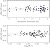 |
Fig. 1 Differential abundance versus excitation potential (upper panel) and differential abundance versus reduced EW (lower panel) for star A relative to the Sun. Filled and empty points correspond to Fe I and Fe II, respectively. The dashed line is a linear fit to the abundance values. |
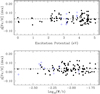 |
Fig. 2 Differential abundance versus excitation potential (upper panel) and differential abundance versus reduced EW (lower panel) for star B relative to the Sun. Filled and empty points correspond to Fe I and Fe II, respectively. The dashed line is a linear fit to the abundance values. |
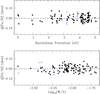 |
Fig. 3 Differential abundance versus excitation potential (upper panel) and differential abundance versus reduced EW (lower panel) for star B relative to A (B − A). Filled and empty points correspond to Fe I and Fe II, respectively. The dashed line is a linear fit to the data. |
4 Results and discussion
The differential abundances of stars A and B relative to the Sun are presented in Figs. 4 and 5. We took the condensation temperatures from the 50% Tc values derived by Lodders (2003). The chemical comparison between one star and the Sun could be affected by GCE effects because of their different (chemical) natal environments (see e.g. Tayouchi & Chiba 2014; Mollá et al. 2015, and references therein). Onthe other hand, we discard GCE effects when mutually comparing stars A and B (owing to their common natal environment), this being an important advantage of the differential method. We corrected GCE effects for (A − Sun) and (B − Sun) by adopting the fitting trends of González Hernández et al. (2013), with a procedure similar to previous works (e.g. Liu et al. 2014; Saffe et al. 2015). Differential abundances are shown with filled points in Figs. 4 and 5, while the two dashed lines are weighted linear fits to all abundance values and only to the refractory species. We used as weight for each chemical element the inverse of the total abundance error σTOT. We also included the solar-twins trend of M 09 using a continuous red line, vertically shifted for comparison.
In this work, we consider as a tentative trend those fits where the slope ranges between 2 and 3σslope, and a significant trend when the slope is greater than 3σslope. The general Tc fit to all species shown in Fig. 4 for the A star presents a slightly negative although non-significant slope (−1.76 ± 2.67 × 10⁻⁵ dex K−1) when compared for example to the solar-twins trend of M 09. The average abundance of the volatile species (Tc < 900 K) is ~0.22 dex, while the average abundance of the refractory species (Tc > 900 K) is ~0.07 dex. On the other hand, the refractory species taken alone do show a clear positive trend (slope of +20.6 ± 4.60 × 10⁻⁵ dex K−1). This corresponds to an excess in refractories when compared to the Sun (which would display a horizontal tendency, not shown) and also when compared to the solar-twins trend of M 09 (red continuous line). Star B shows in Fig. 5 similar behaviour to that shown by the A star in the Fig. 4: a slightly negative although non-significant general slope (−3.46 ± 3.06 × 10⁻⁵ dex K−1) together with a positive trend for refractories (slope of +25.3 ± 5.29 × 10⁻⁵ dex K−1). Therefore, following a reasoning similar to M 09, stars A and B do not seem to be depleted in refractory elements when compared to the solar twins, which is different for the case of the Sun. In other words, terrestrial planet formation would have been less efficient in the stars of this binary system than in the Sun.
The differential abundances of star B using A as reference (B − A) are presented inFig. 6. This plot corresponds to the abundance values derived with the highest possible precision, diminishing errors in the calculation of stellar parameters and GCE effects (e.g. Saffe et al. 2015).
The average differential abundance of the volatile species is ~0.026 dex, while the average of the refractories amounts to ~0.005 dex, showing no clear general trend within the errors (slope of +0.47 ± 2.35 × 10⁻⁵ dex K−1). The refractory elements seem to show a positive Tc slope (+4.05 ± 3.86 × 10⁻⁵ dex K−1), however there is no significant trend due to the relatively large dispersion of the slope. We consider that data with higher quality (perhaps higher S/N) is desirable, because there may be a hidden trend with Tc that the current data cannot discern (average error bars of ~0.05 dex). Following our results, the difference in metallicity for (B − A) is only +0.006 ± 0.009 dex, that is, both stars present almost the same metallicity within our errors. Therefore, both stars present very similar metallicity, and there is no clear difference in the relative content of refractory and volatile elements within our errors. In other words, there is no clear Tc trend between stars A and B, and therefore no clear evidence of terrestrial planet formation in this binary system. Similarly, Liu et al. (2014) concluded that the presence of a giant planet does not necessarily introduce a terrestrial (or rocky) chemical signature into their host stars, by studying the HAT-P-1 binary system. In our case, the massive planet orbiting the A star of the HD 106515 binary system presents a relatively high eccentricity (0.57, Desidera et al. 2012; Marmier et al. 2013). The presence of long-period planets with eccentric orbits was noted by Marmier et al. (2013), who included HD 106515 in their analysis and attributed the origin of the eccentricity to a possible Kozai mechanism. For the case of eccentric giant planets, numerical simulations also found that the early dynamical evolution of giant planets clears out most of the possible terrestrial planets in the inner zone (Veras & Armitage 2005, 2006; Raymond et al. 2011).
We derived stellar parameters for stars A and B by applying both the classical solar-scaled method and the new non-solar-scaled procedure (Saffe et al. 2018). The Δ differences in the parameters taken as (new method − classical method) amount to ΔTeff +27 K, Δlog g + 0.02 dex, Δ[Fe/H] + 0.018 dex, and Δvturb + 0.07 km s−1 for the A star, while for the B star they amount to ΔTeff + 23 K, Δlog g + 0.02 dex, Δ[Fe/H] + 0.012 dex, and Δvturb − 0.34 km s−1. Therefore, for the case of the classical solar-scaled method, we should include in the total error estimation of these parameters a quantity similar to Δ. In this way, considering for example the Teff of stars A and B with classical errors of 57 and 58 K, and adding quadratically the Δ differences of 27 and 23 K, would result in a final total error of 63 and 62 K for stars A and B. In other words, for the stars of this binary system, the use of the new method allows a reduction of ~10% of the total error in Teff.
We note that the new method allows an improvement in the calculation of stellar parameters, while NLTE or GCE corrections only affect the chemical abundances. We present in the Fig. 7 iron abundances versus EWr, using non-solar-scaled opacities but using the solution found in the solar-scaled method. Filled and empty points correspond to Fe I and Fe II, respectively, while the dashed line is a linear fit to the abundance values. Both the presence of an unbalance in this plot, and the fact that Fe II values are greater than Fe I values, shows that the solar-scaled solution (requiring e.g. the excitation and ionization balance of iron lines) is not compatible with the new method. This shows that we can indeed derive a refined solution in stellar parameters when using non-solar-scaled opacities.
We present in Fig. 8 differential abundances versus atomic number using the solar-scaled method (blue circles and lines) and using the new method (red circles and lines) for star B. The same plot for the A star shows a similar behaviour. In the lower panel we present using bars the difference between both procedures (as new method – solar-scaled method), for each chemical species. Some chemical elements are labelled in the plot to facilitate their identification. The lower panel can be considered as an abundance pattern difference obtained when using one method or another. Similar to Saffe et al. (2018), we note that C, O, and S present lower values when using the new method, while the rest of the species mostly present similar or greater abundance values, by an average of ~0.015 dex. The greaterdifference for star B corresponds to La, with a difference near ~0.04 dex. We also present in Fig. 9 a plot similar to Fig. 8, however, in this case for (B − A). Due to the physical similarity between stars A and B, the differences in the individual abundances are usually lower than those of Fig. 8. Most chemical species show almost negligible differences (see lower panel), while some elements show differences of up to ~0.010 dex (for O, K, V, Sr, and Y). Therefore, the differences between both methods are comparable to NLTE corrections or GCE effects and cannot be easily ignored, especially when comparing the stars using the Sun as reference rather than comparing between the stars themselves.
We explored the possibility to use “corrected” solar-scaled models rather than the full non-solar-scaled approach for star B by recomputingsolar-scaled models but using a modified metallicity. We used a corrected metallicity similar to Eq. (3) of Salaris et al. (1993): δ[Fe/H] = log10 (0.638 × 10[α∕Fe] + 0.362), where δ[Fe/H] is the amount of the correction and [α/Fe] is the average of the abundances of the alpha elements. For star B we estimated [α/Fe] ~0.155 dex and δ[Fe/H] ~0.104 dex. The resulting abundances for this correction are presented in Fig. 10. We note in this plot (see e.g. thelower panel) that there is not a perfect match between the abundance values derived with the non-solar-scaled and corrected solar-scaled methods. We suspect that this is due, at least in part, to the fact that solar-scaled models even with corrected [Fe/H] values still made use of solar-scaled opacities when deriving abundances of chemical species other than Fe, giving rise possibly to the small differences observed in Fig. 10.
Differential abundances for stars A and B relative to the Sun, and B relative to A: (A − Sun), (B − Sun), and (B − A).
Refined stellar and planetary parameters derived in this work.
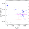 |
Fig. 4 Differential abundances (A − Sun) versus condensation temperature Tc. Dashed lines are weighted linear fits to all and to refractory species, while continuous red lines show the solar-twins trend of M 09 (vertically shifted for comparison). |
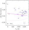 |
Fig. 5 Differential abundances (B − Sun) versus condensation temperature Tc. Dashed lines are weighted linear fits to all and to refractory species, while continuous red lines show the solar-twins trend of M 09 (vertically shifted for comparison). |
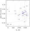 |
Fig. 6 Differential abundances (B − A) versus condensation temperature Tc. Long-dashed lines are a weighted linear fit to all and to the refractory species. The solar-twins trend of M 09 is shown with a continuous red line (vertically shifted for comparison). |
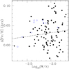 |
Fig. 7 Differential abundances (A − Sun) versus excitation potential using non-solar-scaled opacities, but forced to the solar-scaled solution. Filled and empty points correspond to Fe I and Fe II, respectively. The dashed line is a linear fit to the abundance values. |
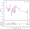 |
Fig. 8 Differential abundances (B − Sun) versusatomic number. Red circles and lines correspond to the solar-scaled method, while blue circles and lines corresponds to the new method. The lower panel presents with bars the difference between both procedures (as new method − solar-scaled method). |
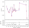 |
Fig. 9 Differential abundances (B − A) vs. atomic number. Red circles and lines correspond to the solar-scaled method, while blue circles and lines corresponds to the new method. The lower panel presents with bars the difference between both procedures (as new method – solar-scaled method). |
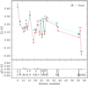 |
Fig. 10 Differential abundances (B − Sun) versus atomic number. Red circles and lines correspond to the non-solar-scaled method, while cyan circles and lines correspond to the other “corrected” solar-scaled method. The lower panel presents with bars the difference between both procedures (as non-solar-scaled − corrected solar-scaled method). |
5 Conclusions
Aiming to detect a possible chemical signature of planet formation, we determined the stellar parameters and chemical pattern in both components of the notable binary system HD 106515, with the highest possible precision. Star A hosts a massive long-period planet whilethere is no planet detected around star B. The strong similarity between both stars greatly diminishes errors in the abundance determination, GCE, or evolutionary effects. We started by deriving the parameters for stars A and B using the Sun as reference, (A − Sun) and (B− Sun), and then we recomputed the parameters for the B star using A as reference, (B − A), obtaining the same results. We derived very similar chemical patterns for stars A and B. By studying the possible temperature condensation Tc trends, we concluded that the stars do not seem to be depleted in refractory elements, which differs from the case of the Sun (Meléndez et al. 2009). However, wesuggest that data with higher quality (perhaps higher S/N) are desirable, because there may be a hidden trend with Tc that the current data cannot discern (average error bars of ~0.05 dex). Then, following the reasoning of Meléndez et al. (2009), the terrestrial planet formation would have been less efficient in the stars of this binary system than in the Sun. In comparing the stars to each other, the lack of clear Tc trend implies that the presence of a giant planet does not necessarily imprint a (terrestrial) chemical signature on its host star, similar to previous results (Liu et al. 2014; Saffe et al. 2015). We note, however, that the A star is orbited by a massive eccentric planet, where numerical simulations found that the early dynamical evolution of giant planets clears out most of the possible terrestrial planets in the inner zone (Veras & Armitage 2005, 2006; Raymond et al. 2011). In this way, both binary systems HD 80606 and HD 106515 do not seem to present a (terrestrial) signature of planet formation (Saffe et al. 2015), with both systems hosting an eccentric giant planet.
For both stars in the binary system, we refined the stellar mass, radius, and age. In particular, we found a notable difference of ~78% in the stellar radius of HD 106515 A compared to the value of Marmier et al. (2013). This difference would seriously affect the derived planetary properties (radius, density) of a potential transiting planet that could be detected by the Transiting Exoplanet Survey Satellite (TESS) mission in the next months. In addition, we refined the minimum planetary mass to mp sini = 9.08 ± 0.20 MJup, which differs by ~6% when compared with the value obtained by Marmier et al. (2013).
We also take the opportunity to compare the parameters derived with non-solar-scaled and classical solar-scaled methods. We obtained a small but noticeable difference in stellar parameters and individual chemical patterns. We showed that using non-solar-scaled opacities, the classical solution cannot verify the standard excitation and ionization balance of iron, similar to Saffe et al. (2018). Also, the difference in abundances between both procedures is comparable to NLTE or GCE effects, especially when using the Sun as reference, and cannot be easily avoided in high-precision studies. Therefore, we encourage the use of non-solar-scaled opacities in studies that require the highest possible precision, such as the detection of a possible chemical signature of planet formation in a binary system.
Acknowledgements
We thank the anonymous referee for constructive comments that improved the paper. The authors wish to recognize and acknowledge the very significant cultural role and reverence that the summit of Mauna Kea has always had within the indigenous Hawaiian community. We are most fortunate to have the opportunity to conduct observations from this mountain. M.F. and F.M.L. acknowledge the financial support from CONICET in the form of Post-Doctoral Fellowships. The authors also thank Drs. R. Kurucz, C. Sneden, and L. Girardi for making their codes available to us.
References
- Adibekyan, V., González Hernández, J., Delgado-Mena, E., et al. 2014, A&A, 564, A15 [Google Scholar]
- Adibekyan, V., Delgado-Mena, E., Figueira, P., et al. 2016, A&A, 592, A87 [NASA ADS] [CrossRef] [EDP Sciences] [Google Scholar]
- Bedell, M., Meléndez, J., Bean, J. L., et al. 2014, ApJ, 795, 23 [NASA ADS] [CrossRef] [Google Scholar]
- Bensby, T., Feltzing, S., & Lundström, I. 2004, A&A, 415, 155 [NASA ADS] [CrossRef] [EDP Sciences] [Google Scholar]
- Bressan, A., Marigo, P., Girardi, L., et al. 2012, MNRAS, 427, 127 [NASA ADS] [CrossRef] [Google Scholar]
- Cumming, A., Marcy, G. W., Butler, R. P. 1999, ApJ, 526, 890 [NASA ADS] [CrossRef] [Google Scholar]
- da Silva, L., Girardi, L., Pasquini, L., et al. 2006, A&A, 458, 609 [NASA ADS] [CrossRef] [EDP Sciences] [Google Scholar]
- Desidera, S., Gratton, R. G., Scuderi, S., et al. 2004, A&A, 420, 683 [NASA ADS] [CrossRef] [EDP Sciences] [Google Scholar]
- Desidera, S., Gratton, R. G., Lucatello, S., & Claudi, R. U. 2006, A&A, 454, 581 [NASA ADS] [CrossRef] [EDP Sciences] [Google Scholar]
- Desidera, S., Gratton, R., Carolo, E., et al. 2012, A&A, 546, A118 [NASA ADS] [CrossRef] [EDP Sciences] [Google Scholar]
- ESA 1997, VizieR Online Data Catalog: I/239 [Google Scholar]
- Gaia Collaboration (Brown, A. G. A., et al.) 2018, A&A, 616, A1 [NASA ADS] [CrossRef] [EDP Sciences] [Google Scholar]
- Girardi, L., Bressan, A., Bertelli, G., & Chiosi, C. 2000, VizieR Online Data Catalog: J/A+AS/141/371 [Google Scholar]
- González Hernández, J., Delgado Mena, E., Sousa, S. G., et al. 2013, A&A, 552, A6 [NASA ADS] [CrossRef] [EDP Sciences] [Google Scholar]
- Høg, E., Fabricius, C., Makarov, V. V., et al. 2000, A&A, 355, L27 [Google Scholar]
- Johansson, S., Litzén, U., Lundberg, H., & Zhang, Z. 2016, ApJ, 584, L107 [Google Scholar]
- Korotin, S. A., Andrievsky, S., Hansen, C., et al. 2015, A&A, 581, A70 [NASA ADS] [CrossRef] [EDP Sciences] [Google Scholar]
- Kurucz, R. L. 1993, ATLAS9 Stellar Atmosphere Programs and 2 km s−1 grid, Kurucz CD-ROM No. 13 (Cambridge, MA: Smithsonian Astrophysical Observatory) [Google Scholar]
- Kurucz, R., & Bell, B. 1995, Atomic Line Data, Kurucz CD-ROM No. 23, (Cambridge, MA: Smithsonian Astrophysical Observatory) [Google Scholar]
- Lambert, D. L. 1978, MNRAS, 182, 249 [NASA ADS] [CrossRef] [Google Scholar]
- Laws, C., & Gonzalez, G. 2016 ApJ, 553, 405L [Google Scholar]
- Liu, F., Asplund, M., Ramírez, I., Yong, D., & Meléndez, J. 2014, MNRAS, 442, L51 [NASA ADS] [CrossRef] [Google Scholar]
- Lodders, K. 2003, AJ, 591, 1220 [Google Scholar]
- Mack, C., Schuler, S., Stassun, K., et al. 2014, ApJ, 787, 98 [NASA ADS] [CrossRef] [Google Scholar]
- Marmier, M., Segransan, D., Udry, S., et al. 2013, A&A, 551, A90 [NASA ADS] [CrossRef] [EDP Sciences] [Google Scholar]
- Mayor, M., Marmier, M., Lovis, C., et al. 2011, ArXiv e-prints [arXiv:1109.2497] [Google Scholar]
- Meléndez, J., Asplund, M., Gustafsson, B., & Yong, D. 2009, AJ, 704, L66 [Google Scholar]
- Meléndez, J., Ramírez, I., Karakas, A., et al. 2014, AJ, 791, 14 [Google Scholar]
- Mollá, M., Cavichia, O., & Gibson, B. 2015, MNRAS, 451, 3693 [NASA ADS] [CrossRef] [Google Scholar]
- Nissen, P. E., Silva Aguirre, V., Christensen-Dalsgaard, J., et al. 2017, A&A, 608, A112 [NASA ADS] [CrossRef] [EDP Sciences] [Google Scholar]
- Ramírez, I., Allende Prieto, C., & Lambert, D. 2007, A&A, 465, 271 [NASA ADS] [CrossRef] [EDP Sciences] [Google Scholar]
- Ramírez, I., Meléndez, J., & Asplund, M. 2009, A&A, 508, L17 [NASA ADS] [CrossRef] [EDP Sciences] [Google Scholar]
- Ramírez, I., Asplund, M., Baumann, P., Meléndez, J., & Bensby, T. 2010, A&A, 521, A33 [NASA ADS] [CrossRef] [EDP Sciences] [Google Scholar]
- Ramírez, I., Meléndez, J., Cornejo, D., Roederer, I., & Fish, J. 2011, AJ, 740, 76 [CrossRef] [Google Scholar]
- Raymond, S., Armitage, P., Moro-Martín, A., et al. 2011, A&A, 530, A62 [NASA ADS] [CrossRef] [EDP Sciences] [Google Scholar]
- Saffe, C. 2011, Rev. Mex. Astron. Astrofis., 47, 3 [NASA ADS] [Google Scholar]
- Saffe, C., Flores, M., & Buccino, A. 2015, A&A, 582, A17 [NASA ADS] [CrossRef] [EDP Sciences] [Google Scholar]
- Saffe, C., Flores, M., Jaque Arancibia, M., Buccino, A., & Jofré, E. 2016, A&A, 588, A81 [NASA ADS] [CrossRef] [EDP Sciences] [Google Scholar]
- Saffe, C., Jofré, E., Martioli, E., et al. 2017, A&A, 604, L4 [NASA ADS] [CrossRef] [EDP Sciences] [Google Scholar]
- Saffe, C., Flores, M., Miquelarena, P., et al. 2018, A&A, 620, A54 [NASA ADS] [CrossRef] [EDP Sciences] [Google Scholar]
- Salaris, M., Chieffi, A., & Straniero, O. 1993, ApJ, 414, 580 [NASA ADS] [CrossRef] [Google Scholar]
- Schuler, S., Cunha, K., Smith, V., et al. 2011, ApJ, 737, L32 [NASA ADS] [CrossRef] [Google Scholar]
- Shi, J. R., Gehren, T., & Zhao, G. 2004, A&A, 423, 683 [NASA ADS] [CrossRef] [EDP Sciences] [Google Scholar]
- Sneden, C. 2016, ApJ, 184, 839 [Google Scholar]
- Takeda, Y. 2005, PASJ, 57, 83 [NASA ADS] [Google Scholar]
- Tayouchi, D., & Chiba, M. 2014, AJ, 788, 89 [NASA ADS] [CrossRef] [Google Scholar]
- Teske, J., Schectman, S., Vogt, S., et al. 2016a, AJ, 152, 167 [NASA ADS] [CrossRef] [Google Scholar]
- Teske, J., Khanal, S., & Ramírez, I. 2016b, ApJ, 819, 19 [NASA ADS] [CrossRef] [Google Scholar]
- Tucci Maia, M., Meléndez, J., & Ramírez, I. 2014, ApJ, 790, L25 [NASA ADS] [CrossRef] [Google Scholar]
- Veras, D., & Armitage, P. 2005, ApJ, 620, L111 [NASA ADS] [CrossRef] [Google Scholar]
- Veras, D., & Armitage, P. 2006, ApJ, 645, 1509 [NASA ADS] [CrossRef] [Google Scholar]
- Vogt, S. S., Allen, S. L., Bigelow, B. C., et al. 1994, SPIE, 2198, 362 [Google Scholar]
CORALIE is not an actual acronym. CORALIE was instead named after the baby daughter of an engineer from the Observatoire de Haute-Provence in France.
IRAF is distributed by the National Optical Astronomical Observatories, which is operated by the Association of Universities for Research in Astronomy, Inc. under a cooperative agreement with the National Science Foundation.
By “full” we mean that line-by-line differences were considered in both the derivation of stellar parameters and (not only) abundances.
We used the standard notation [X/Fe] = [X/H] − [Fe/H].
Value currently reported in The Extrasolar Planets Encyclopaedia.
All Tables
Differential abundances for stars A and B relative to the Sun, and B relative to A: (A − Sun), (B − Sun), and (B − A).
All Figures
|
Fig. 1 Differential abundance versus excitation potential (upper panel) and differential abundance versus reduced EW (lower panel) for star A relative to the Sun. Filled and empty points correspond to Fe I and Fe II, respectively. The dashed line is a linear fit to the abundance values. |
| In the text | |
|
Fig. 2 Differential abundance versus excitation potential (upper panel) and differential abundance versus reduced EW (lower panel) for star B relative to the Sun. Filled and empty points correspond to Fe I and Fe II, respectively. The dashed line is a linear fit to the abundance values. |
| In the text | |
|
Fig. 3 Differential abundance versus excitation potential (upper panel) and differential abundance versus reduced EW (lower panel) for star B relative to A (B − A). Filled and empty points correspond to Fe I and Fe II, respectively. The dashed line is a linear fit to the data. |
| In the text | |
|
Fig. 4 Differential abundances (A − Sun) versus condensation temperature Tc. Dashed lines are weighted linear fits to all and to refractory species, while continuous red lines show the solar-twins trend of M 09 (vertically shifted for comparison). |
| In the text | |
|
Fig. 5 Differential abundances (B − Sun) versus condensation temperature Tc. Dashed lines are weighted linear fits to all and to refractory species, while continuous red lines show the solar-twins trend of M 09 (vertically shifted for comparison). |
| In the text | |
|
Fig. 6 Differential abundances (B − A) versus condensation temperature Tc. Long-dashed lines are a weighted linear fit to all and to the refractory species. The solar-twins trend of M 09 is shown with a continuous red line (vertically shifted for comparison). |
| In the text | |
|
Fig. 7 Differential abundances (A − Sun) versus excitation potential using non-solar-scaled opacities, but forced to the solar-scaled solution. Filled and empty points correspond to Fe I and Fe II, respectively. The dashed line is a linear fit to the abundance values. |
| In the text | |
|
Fig. 8 Differential abundances (B − Sun) versusatomic number. Red circles and lines correspond to the solar-scaled method, while blue circles and lines corresponds to the new method. The lower panel presents with bars the difference between both procedures (as new method − solar-scaled method). |
| In the text | |
|
Fig. 9 Differential abundances (B − A) vs. atomic number. Red circles and lines correspond to the solar-scaled method, while blue circles and lines corresponds to the new method. The lower panel presents with bars the difference between both procedures (as new method – solar-scaled method). |
| In the text | |
|
Fig. 10 Differential abundances (B − Sun) versus atomic number. Red circles and lines correspond to the non-solar-scaled method, while cyan circles and lines correspond to the other “corrected” solar-scaled method. The lower panel presents with bars the difference between both procedures (as non-solar-scaled − corrected solar-scaled method). |
| In the text | |
Current usage metrics show cumulative count of Article Views (full-text article views including HTML views, PDF and ePub downloads, according to the available data) and Abstracts Views on Vision4Press platform.
Data correspond to usage on the plateform after 2015. The current usage metrics is available 48-96 hours after online publication and is updated daily on week days.
Initial download of the metrics may take a while.