| Issue |
A&A
Volume 625, May 2019
|
|
|---|---|---|
| Article Number | A45 | |
| Number of page(s) | 8 | |
| Section | Interstellar and circumstellar matter | |
| DOI | https://doi.org/10.1051/0004-6361/201833979 | |
| Published online | 07 May 2019 | |
Modeling of CoRoT and Spitzer lightcurves in NGC 2264 caused by an optically thick warp
1
Departamento de Astronomía, Universidad de Guanajuato,
Callejón de Jalisco S/N,
Guanajuato,
Gto. 36240,
México
e-mail: This email address is being protected from spambots. You need JavaScript enabled to view it.
2
IPAG, Université Grenoble Alpes,
38000
Grenoble,
France
e-mail: This email address is being protected from spambots. You need JavaScript enabled to view it.
Received:
28
July
2018
Accepted:
19
March
2019
Abstract
Aims. We present an analysis of simultaneously observed CoRoT and Spitzer lightcurves for four systems in the stellar forming region NGC 2264: Mon-660, Mon-811, Mon-1140, and Mon-1308. These objects share in common a strong resemblance between the optical and infrared lightcurves, such that the mechanism responsible for producing them is the same. The aim of this paper is to explain both lightcurves simultaneously with only one mechanism.
Methods. We modeled the infrared emission as coming from a warp composed of an optically thick wall and an optically thick asymmetric disk beyond this location. We modeled the optical emission mainly by partial stellar occultation by the warp.
Results. The magnitude amplitude of the CoRoT and Spitzer observations for all the objects can be described with the emission coming from the system components. The difference between them is the value of the disk flux compared with the wall flux and the azimuthal variations of the former. This result points out the importance of the hydrodynamical interaction between the stellar magnetic field and the disk.
Conclusions. CoRoT and Spitzer lightcurves for the stellar systems Mon-660, Mon-811, Mon-1140, and Mon-1308 can be simultaneously explained using the emission coming from an asymmetric disk and emission with stellar occultation by an optically thick wall.
Key words: accretion, accretion disks / stars: pre-main sequence
© ESO 2019
1 Introduction
The flux variability of young stellar objects (YSOs) is commonly detected in the optical and in the infrared. For the young stellar cluster NGC 2264 there are several observational studies that clearly show variability for a large fraction of the observed objects: in the optical with the CoRoT Space Telescope (Alencar et al. 2010; Cody et al. 2014; Stauffer et al. 2015, 2016) and in the infrared with the Spitzer Space Telescope (Morales-Calderón et al. 2011; Cody et al. 2014; Stauffer et al. 2015, 2016). Stauffer et al. (2016) focus on a sample of stellar stochastic lightcurves that can be explained with changes in Ṁ that lead to a variable dust heating of the material rotating around the object. Some of the objects show the infrared (IR) and optical lightcurves resembling each other, suggesting that the physical mechanism responsible for their shape is the same.
In NGC 2264, Alencar et al. (2010) use CoRoT lightcurves to search for a subsample with a periodic signal that can be explained with occultations by an inner warp as in AA Tau (Bouvier et al. 1999). They conclude that at least approximately 30–40% of YSOs with inner dusty disks present this kind of behavior. In the Orion Nebula Cluster, Morales-Calderón et al. (2011) present Spitzer lightcurves at 3.6 and 4.5 μm of 41 objects that show flux drops with a duration of one to a few days, which can be interpreted with material crossing the line of sight. From this set, they extract one third with a detected periodic dip, pointing out that structures moving at a keplerian angular velocity are obvious features shaping the lightcurves. For this same region, Rice et al. (2015) confirm that 73 out of a sample of 1203 objects present AA Tau-type periodic lightcurves.
Bouvier et al. (1999) suggest that such structures can be associated with the accretion of material along the stellar magnetic field lines, where the magnetic dipolar axis is inclined with respect to the disk rotational axis. The magneto-hydrodynamical (MHD) simulations of this system configuration by Romanova et al. (2013) show besides the magnetospheric streams an uniformly rotating bending wave located between the location of the streams and the outer vertical resonance. Both components can shadow the star when the system is seen at high inclination, thus becoming a physical mechanism to explain the lightcurves’ shape. A theoretical analysis of the MHD equations by Terquem & Papaloizou (2000) also arrives at the conclusion that a shadowing warp is formed.
Inner disk structure can explain azimuthal surface brightness asymmetry in the object TW Hya, which moves at a constant angular velocity consistent with shadowing material rotating at a keplerian velocity associated with a radius around 1AU (Debes et al. 2017). Also inhomogeneities very close to the star are responsible for the shape of the optical and IR lightcurves in the young low-mass star ISO-Oph-50 (Scholz et al. 2015). From the observations of the IC 348 cluster, Flaherty et al. (2012) point out three low luminosity objects (LRLL 58,67,1679) with non-periodic lightcurves in the near-IR (NIR) that can be interpreted with dust that moves along the stellar magnetic field lines.
From this, we can conclude that the material distributed asymmetrically in the innermost region of the disk is relevant to explain the variability of the lightcurves either in the optical or in the IR, as can be seen from the aforementioned observational studies and from the theoretical works that sustain this information. In this work on the interpretation of the variability of the lightcurves, we point out for each object the importance of the disk flux compared with the wall flux and the amplitude for the azimuthal contribution of the former. This allows us to qualitatively characterize the innermost disk structure that we cannot resolve with current instrumentation. This characterization is important because there are many observed planets located very close to the star and their evolution towards this location strongly depends on the physical conditions of the disk inner part in the initial stage of the system’s life.
McGinnis et al. (2015) studied the photometric variability of YSOs in the star-forming region NGC 2264. They present CoRoT lightcurves for 33 objects showing AA Tau-type behavior: the optical lightcurve can be described with periodical stellar occultations due to an optically thick warp. From this set, McGinnis et al. (2015) present simultaneous observations of 29 stars in the optical and the infrared using the CoRoT and the Spitzer Space Telescopes. A comparison between the lightcurves at both wavelength ranges shows different behavior. In this study, we will focus on the four objects that present AA Tau-like modulation in the IR and in the optical, which closely follow each other, meaning that the mechanisms that are generating the variability in the optical and in the IR are related. The objects are Mon-660, Mon-811, Mon-1140, and Mon-1308.
The aim of this work is to consistently reproduce the observed amplitude of the CoRoT magnitude Δ[CoRoT], along with the observed amplitudes in the IR: Δ[3.6] and Δ[4.5]. The material that it is occulting the star and that is responsible for the changes in [CoRoT] is that producing the excess in the IR range, and is thus responsible for changes at [3.6] and [4.5]μm.
A parametric study about the effect of a dust distribution around a star in optical and IR lightcurves was previously done by Kesseli et al. (2016). They used a Monte Carlo radiation transfer code described in Whitney et al. (2013) that includes heating by stellar radiation and by accretion. Besides the dust emission, Kesseli et al. (2016) include hotspots at different latitudes to produce different amounts of magnitude variability due to stellar rotation. Their models qualitatively reproduce the periodic dippers analyzed in McGinnis et al. (2015) using a disk warp that changes in radius and in azimuthal angle (see Eq. (8) in Whitney et al. 2013) in a way similar to the 2D warp shape used in Bouvier et al. (1999) for the interpretation of the optical lightcurve of AA Tau. Our idea is to follow the same analysis but applied to specific objects.
In Sect. 2 we present the description of the modeling, followed in Sect. 3 by the results of the lightcurve modeling for the set of four YSOs. Section 4 contains the discussion and finally Sect. 5 gives the conclusions.
2 Modeling
2.1 Main aspects of the modeling
The disk surrounding the star has two main components: an optically thick vertical wall and an asymmetrical emitting structure beyond this location. These two components merge to form the warp (see Fig. 1 for a sketch of the system). The optically thick vertical wall is located at the Keplerian radius, RK, which is consistent with the observed period of the lightcurve. We assume that the main mechanism shaping the wall is magnetospheric accretion at the magnetospheric radius (Rmag) such that RK ~ Rmag.
Thus, itis reasonable to assume the presence of a wall, and, as a zero order approach, we consider a stationary disk configuration that is perturbed to form the vertical wall. At the wall location, we expect a highly dynamical environment due to the MHD interaction between the disk and the stellar magnetosphere such that the stationary disk configuration is not physically correct. In the context of this work, this configuration is used to give characteristic values to the density and the vertical distribution of grain sizes. These values are required to get the wall temperature (Twall), but it mainly depends on the distance to the star, thus, the values taken do not significantly change the modeled wall emission. In Fig. 2 we present Twall in terms of height for the stellar objects Mon-660, Mon-811, and Mon-1308. We do not include the plot for Mon-1140 because this object does not have a dusty wall (see Sect. 3.3 for details). We expect in reality that the material distribution in this region is much more complex than the toy model used here as is shown in the analysis of the young low-mass star ISO-Oph-50, where the modeling by Scholz et al. (2015) requires inhomogeneities in the inner disk that can be the result of a turbulent environment. In any case, we also think that an optically thick structure is responsible for the main features of the lightcurves analyzed in this paper.
There is dust inside the magnetosphere when the sublimation radius Rsub < Rmag. Due to the stellar magnetic field lines, this dust is not located in a stationary disk, thus it is not easily characterized. In terms of the modeling, the emission coming from the material (gas plus dust) inside the magnetosphere and from the outer disk is set by the flux required to explain the observed IR flux and the amount of variability in the Spitzer lightcurves. Emission from gas inside the sublimation radius is suggested in the interferometric observations of Herbig Ae stars MWC 275 and AB Aur (Tannirkulam et al. 2008). In order to explain the observations, the flux should account for 40–60% of the total K-band emission. Akeson et al. (2005) found the same result for the T Tauri star RY Tau. However, McClure et al. (2013) conclude from the fitting of the NIR emission of a sample of T Tauri stars that there is no evidence of emission from optically thick gas inside the sublimation radius.
In order to confirm the existence or not of dust inside the magnetosphere, we calculate Rsub as in Nagel et al. (2013) assuming that the large grains are located in the disk midplane. In the boundary between the dusty and dust-free disk, there is a large opacity change such that an optically thick structure is formed. The temperature of this structure (Twall) is calculated starting from the stellar radius and increasing the value up to the radius where Twall = Tsub. The radius where this condition is fulfilled is Rsub. The value of Twall is calculated with the analytical expression given in Nagel et al. (2013). The value Tsub is a function of gas density and it is taken for different grain species from Table 3 in Pollack et al. (1994). The gas density is taken assuming as typical the density of a stationary configuration for a settled disk. The density structure is taken using the codes in D’Alessio et al. (1998). The dust is distributed in the disk using two grain size distributions: one for large grains close to the midplane and another for small grains in the upper layers. The transition between these two distributions is modeled as in D’Alessio et al. (2006).
As we fully explain in Sect. 2.3, the height of the vertical wall is fixed by estimating the amount of occultation required to explain the CoRoT lightcurves. Physically this is possible because the highly dynamical interaction in this region allows the movement of the large grains located in the midplane layer in the stable state (turning off the magnetic stellar field) toward greater heights. We also note that this is in accord with the interpretation of the observations of Mon-660 by Schneider et al. (2018), where in order to interpret some optical spectra, an optically thick wall is required that produces complete occultation of a fraction of the stellar surface fC, an optically thin wall that makes extinct another fraction of this surface fB, and finally an unocculted fraction fA: fA + fB + fC = 1. Besides, Schneider et al. (2018) model also requires an increment on the abundance of dust grains in the optically thin layer that can be obtained with the dust that arrives due to the hydrodynamical perturbation.
For Mon-660, Schneider et al. (2018) estimate the gas density in the extinct region, which is above the optically thick wall. They use an analysis of the Na and K optical doublets to derive an absorbing column density for these species, which corresponds to a hydrogen density equal to 2 × 1019 cm−2. The disk warp is located at 0.1 AU and they assume a radial thickness along the line of sight of the same magnitude, ending with a volumetric density nH ~ 107 cm−3 in terms of mass, ρextinc = 1.67 × 10⁻¹⁷ gcm−3. This density is responsible for the extinction of the fraction fB of the stellar surface. If we run models using this value for the density in a layer above the optically thick wall, then we conclude that the contribution to the IR flux can be neglected. Thus, we do not include this optically thin component in our modeling of the IR lightcurves.
The grain size distribution (n(a)) is taken from Mathis (1977) as typical for the interstellar medium (ISM), which is extensively used in protoplanetary disks: n(a) ~ a−3.5. The size range for the small grains located in the upper layers of the wall is amin = 0.005 μm and amax = 0.25 μm. For the larger grains located close to the midplane, amin = 0.005 μm and amax = 1 mm. The dust mass fractions compared to the gaseous mass are ζsil = 0.004 and ζgrap = 0.0025 for the silicate and the graphite components, respectively.
The MHD simulations by Kulkarni & Romanova (2013) show that the perturbation on the disk is not only located close to Rmag but can move further out on the disk. The structure of this region is highly complex but for the sake of the simple modeling presented here, this outer zone contributes with an asymmetrical flux parameterized as in Sect. 2.2. The MHD simulations of a tilted stellar magnetic field interacting with a disk made by Romanova et al. (2013) focus on the formation of waves in the disk. They conclude that a bending wave (out-of-plane modes) is formed between the corotational resonance (located at the corotational radius Rcr) and the outer vertical resonance located at Rovr = 41∕3Rcr. In our case, Rcr = Rk = Rmag such that the bending wave is the structure responsible for the emission of the outer component of the warp. We estimate its emission as the missing contribution required to explain the Spitzer lightcurves (see Sect. 2.2). This whole structure corotates with the magnetosphere such that it is relevant to explain the periodic lightcurves.
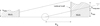 |
Fig. 1 Sketch of the system modeled. The inclined straight lines represent two lines of sight with the same inclination crossing different sections of the system. The left line contributes to emission of the wall and the right line contributes to emission of the disk. In this case, all the stellar surface is occulted. |
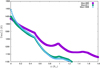 |
Fig. 2 Wall temperature (Twall in Kelvin) atthe vertical wall as a function of height (z in stellar radius) for Mon-660, Mon-811, and Mon-1308. |
2.2 Emitted flux
The flux observed is modeled using
 (1)
(1)
where Fwall is the flux coming from the wall, Fdisk is the flux coming from the region beyond the wall, and F⋆ is the flux coming from the unocculted star.
The emission from the optically thick wall comes from its atmosphere, and the radiation is extinguished with the material between this location and the observer. Each layer of the atmosphere (located at an optical depth τ) is emitting as a blackbody at a temperature given as in D’Alessio et al. (2005),
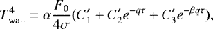 (2)
(2)
where α = 1 − w, w is the mean albedo to the stellar radiation,  ,
,  is the stellar flux that heats the wall at the radius Rwall, and σ is the Steffan-Boltzmann constant. The variables
  ,
,  ,
,  , q, and w depend on the mean Planck opacities (absorption and scattering), one set of them calculated using the typical wavelength range of the stellar radiation and the other set calculated using the typical wavelength range of the disk radiation. The scattering of stellar radiation is assumed to be isotropic. Thus, the total wall flux at each frequency (ν) is calculated as an integral over the solid angle Ω subtended by the wall and over the optical depth τ,
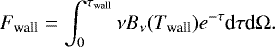 (3)
(3)
The emission comes from the wall atmosphere, which is defined with the optical depth τ, where τ = 0 in the surface of the wall and increases towards larger radius until τ = τwall = 1.5.
The emitted flux coming from the disk in the IR (3.6 or 4.5) is parameterized as
 (4)
(4)
which is consistent with the warp shape described in Eq. (6), where ϕ0 is the phase with the lowest flux contribution. Because the behavior at 3.6 and 4.5 μm is analogous, we focus on 4.5 μm when referring to IR emission, such that the aim is to explain the 4.5 μm Spitzer lightcurve. Physically, this corresponds to a structure that moves with the same periodicity as the wall. The symbol ϕ corresponds to the phase of the lightcurves, δ is a free parameter fitted to explain the amplitude of the observed [4.5] (Δ[4.5]), and ⟨ Fdisk⟩ is the mean disk flux required to be consistent with the mean flux extracted from the IR lightcurves (⟨ Fobs⟩). This value is fixed using the equation
 (5)
(5)
where ⟨Fwall⟩ is the mean value of the IR emission coming from the wall. The δ value parameterizes the azimuthal variation of Fdisk. We associate this variation to the hydrodynamical waves formed by the interaction between the stellar magnetic field and the disk. If δ increases then the effective area of the wave that it is facing the observer increases, as does the flux emitted by the structure.
2.3 Warp geometry
The optically thick part of the warp is required to block some of the stellar radiation. This structure is asymmetric, with a height given by hwarp. The axisymmetric part of the structure consists of a wall with height hmin. The values for hwarp are taken from the warp model of Bouvier et al. (1999) and used by Fonseca et al. (2014) for Mon-660,
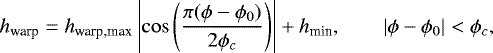 (6)
(6)
 (7)
(7)
where we include the axisymmetric section. We checked that the height hmin is not eclipsing any section of the star in order to be consistent with the models in McGinnis et al. (2015). This height also satisfies hmin ∕R ~ 0.1, which is a typical value for thin protoplanetary disks. We note that hwarp,max + hmin is the largest warp height in the models by McGinnis et al. (2015).
When the maximum height of the warp, hwarp,max + hmin, is along the line of sight then the optical lightcurve reaches the largest magnitude (lowest flux). For a given inclination i, one can find the value for hwarp,max, which is necessary to explain the observed (Δ[CoRoT]). The value hwarp is increased by 0.05 steps inorder to find hwarp,max. For all the objects, the pairs are given in Appendix A.
2.4 Modeling ingredients
We use the flux calculated as described in Sect. 2.2 to estimate [CoRoT] and [4.5]. We arbitrarily set the lowest magnitude as zero for both wavelengths. Thus, Δ[CoRoT] and Δ[4.5] are calculated with respect to this point. For each pair (hwarp,max,i), we have tworemaining free parameters that can be varied in order to explain the magnitude variability in the IR, Δ[4.5]. The parameter δ (see Sect. 2.2) is the one used to fit Δ[4.5]. A larger value of δ implies a larger value for Δ[4.5], thus we increase (or decrease) the value until the observed Δ[4.5] is reached. This process can be done for each object and for each pair (hwarp,max,i) to find a fit. In Sect. 3, we present the plot for the case i = 77°, and in Table 2 we show the value of δ obtained for each pair (hwarp,max,i). This table shows the degeneracy of the modeling and because the physical processes shaping the disk are not fully known, we cannot favor one solution over another. Our aim is to find the order of magnitude of δ such that we can conclude something about the degree of asymmetry of the inner disk. In order to break the degeneracy, detailed MHD simulations including radiative transfer should be done and compared with resolved observations of the inner part of the disk to extract a value for δ and relate it to the actual disk height. Observationally i can be fixed such that the modeling can be restricted to such a case. The parameter ϕc determines the azimuthal range where hwarp = hmin, such that it is related to the shape of the CoRoT lightcurve. A range of ϕc are given by McGinnis et al. (2015) in the modeling of the lightcurves of the systems analyzed here. The value used here is within this range and fixed to the value ϕc = 180°. A study changing this parameter is worth carrying out when the goal is to explain the details of the lightcurves. The pursuit of this requires a full understanding of all the physical processes involved based on a complete sample of hydrodynamical simulations, which requires a great amount of computational resources; this is not the aim of the current work.
Stellar parameters.
3 Lightcurve modeling
3.1 Modeling of Mon-660
This object was previously known as V354 Mon. Fonseca et al. (2014) interpreted its CoRoT lightcurve as being due to occultations by an optically thick warp with a sinusoidal shape, like the model Bouvier et al. (1999) used for the interpretation of the lightcurve of AA Tau. Observations in 2008 and 2011 are consistent with a stellar rotational period of Prot = 5.25 days. The keplerian radius consistent with this period is Rk = 7.64 R⋆. An explanation for the timescale of the variability requires that the material responsible for it should be located around this location. We remember that a bending wave located between Rk = Rcr and Rovr moves with this periodicity, thus it can be responsible for the stellar occultation and IR emission.
The stellar parameters are given in Table 1. The minimum sublimation radius is Rsub,min = 7.70 R⋆ using Ṁ = 3 × 10⁻⁹ M⊙ yr−1. This value corresponds to the mean of log (Ṁ) taken from Venuti et al. (2014). We note that Rsub,min is slightly larger than Rk; because of the uncertainties we assume that the dusty wall is located at Rk.
As mentioned in Sect. 2.3, Table A.1 presents the set of pairs (i, hmax) explaining the observed Δ[CoRoT] ~ 0.8. The value of δ that allows us to explain the observed Δ[4.5] ~ 0.3 mag (McGinnis et al. 2015) for each pair and the mean observed flux at 4.5 μm (⟨ Fobs⟩) is given in Table 2. The observed values for Δ[4.5] and Δ[CoRoT] are the maxima.
In Fig. 3 we present the modeled and observed lightcurves for i = 77° with Hmin = 0.7R⋆. We calculate a mean of the lightcurves, adding all the photometric cycles, such that all the observed points are used. We give the standard deviation σ as a measure of the dispersion of the data, which is simply an effect of the variability of the lightcurves with respect to the mean curve. As a reference for the maximum amplitude observed, we plot the + 1σ lightcurves and fit their amplitudes. The flux contributions from each component are presented in Fig. 4. In the optical, the contribution from the wall and from the disk can be neglected, thus it is not shown.
Parameters in the models.
3.2 Modeling of Mon-811
From observations in 2011, Prot = 7.88 days. The keplerian radius consistent with this period is Rk = 8.19 R⋆. The stellar parameters are given in Table 1. The minimum sublimation radius is Rsub,min = 6.19 R⋆ using Ṁ = 3 × 10⁻⁹ M⊙yr−1. This value corresponds to the mean of log (Ṁ) taken from Venuti et al. (2014).
As mentioned in Sect. 2.3, Table A.1 presents the set of pairs (i,hmax) explaining the observed Δ[CoRoT] = 0.5. The value of δ that allows us to explain the observed Δ[4.5] ~ 0.2 mag (McGinnis et al. 2015) for each pair and ⟨Fobs⟩ is given in Table 2. In Fig. 5 we present the modeled and observed lightcurves for i = 77° with Hmin = 0.8 R⋆. The flux contributions from each component are presented in Fig. 6.
3.3 Modeling of Mon-1140
From observations in 2008 and 2011, Prot = 3.87 and 3.9 days, respectively. The keplerian radius consistent with the latter period is Rk = 6.75 R⋆. The stellar parameters are given in Table 1. The minimum sublimation radius is Rsub,min = 7.93 R⋆ using Ṁ = 7.76 × 10⁻⁹ M⊙ yr−1. The value for Ṁ is taken from Venuti et al. (2014). They present two different estimates of Ṁ and we decided to take the value with the lowest Rsub,min. However, even in this case Rsub,min > Rk and we can conclude that there is no dust at Rk = Rmag, such that no wall is formed by magnetospheric streams. For this object, the bending wave and/or material above it is responsible for the stellar occultation. It is noteworthy that the value for ⟨ Fdisk⟩ calculated using Eq. (5) is a few times smaller than required to explain the observed Δ[4.5]. Thus, for this object the IR lightcurves are interpreted only using the emission coming from the disk, such that instead of Eq. (5) we use ⟨ Fobs⟩ = ⟨Fdisk⟩. The value of δ that allows us to explain the observedΔ[4.5] ~ 0.1 mag (McGinnis et al. 2015)and ⟨Fobs⟩ is given in Table 2. In Fig. 7 we present the modeled and observed [4.5] lightcurves. For the modeling of this object, a change in i means that the physical configuration required to obtain Fdisk changes. The analysis of this changing disk configuration is not pursued in this work. The optical lightcurves presented correspond to a vertical wall located at Rsub,min, with the height given by hwarpRsub,min∕Rk. The geometrical characterization of the bending wave is not the aim of this work. The flux contributions from each component are presented in Fig. 8.
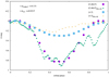 |
Fig. 3 Modeled optical and 4.5 μm lightcurves for Mon-660 at i = 77°. The modeled CoRoT lightcurve is represented by filled circles, and the modeled Spitzer photometric magnitudes at 4.5 μm are plotted as solid squares. For comparison the observed + 1σ CoRoT (points) and the + 1σ Spitzer 4.5 μm (asterixs) lightcurves are presented. We use all the cycles presented in McGinnis et al. (2015) to calculate the observed curves. At the upper left corner, we show the value for the mean standard deviation for the CoRoT and Spitzer data. |
3.4 Modeling of Mon-1308
From observations in 2008 and 2011, Prot = 6.45 and 6.68 days. The keplerian radius consistent with this period is Rk = 7.81 R⋆. The stellar parameters are given in Table 1. The minimum sublimation radius is Rsub,min = 5.45 R⋆ using Ṁ = 8.51 × 10⁻⁹ M⊙ yr−1. The value for Ṁ is taken from Venuti et al. (2014).
As mentioned in Sect. 2.3, Table A.1 presents the set of pairs (i, hmax) explaining the observed Δ[CoRoT] = 0.4. The value of δ that allows us to explain the observed Δ[4.5] ~ 0.4 mag (McGinnis et al. 2015) for each pair and ⟨Fobs⟩ is given in Table 2. In Fig. 9 we present the modeled and observed lightcurves for i = 77° with Hmin = 0.8 R⋆. The flux contributions from each component are presented in Fig. 10.
4 Discussion
The Spitzer lightcurves for the objects Mon-660, Mon-811, and Mon-1308 can be explained using the emission coming from the star, the vertical wall, and the asymmetrical emission associated with a disk behind the wall. The wall is located at the keplerian radius consistent with the period of the lightcurves. The asymmetry of this structure is the result of the interaction between a stellar magnetic field with a tilted dipolar axis and the disk. For Mon-1140, at the location of the wall, the stellar heating sublimates the dust such that the IR lightcurves are explained only with the stellar and the disk emission.
The CoRoT lightcurves for Mon-660, Mon-811, and Mon-1308 are interpreted with occultation for a vertical wall, however, forMon-1140 there is no wall so the occulting structure should lie in the asymmetrical disk. The MHD simulations in Romanova et al. (2013) suggest that vertical perturbations in the disk can be responsible for the stellar shadowing. The real fact is that dust should be moved upward in order to periodically block a section of the stellar surface.
Romanova et al. (2013) describe the resulting configuration for the interaction between the stellar magnetosphere and the disk as a bending wave that is located between the corotation radius (Rcr) and the location for the outer vertical resonance (Rovr = 41∕3Rcr). For rapidly rotating stars, Rcr = Rmag is close to the rotational equilibrium state, which is a state commonly reached by accreting magnetized stars (Long Romanova & Lovelace 2005). In our case, Rk = Rmag such that Rk = Rcr. The wave located in this radial range moves at the stellar period such that any section of it can be responsible for the stellar occultations required to explain the CoRoT lightcurves. Because the emission of such a structure is beyond the scope of this paper, we simply quantify its emission as the missing contribution required to explain the Spitzer lightcurves (see Sect. 2.2).
The value for δ required to explain the Spitzer lightcurves is the largest for the systems with the largest Δ[4.5]: Δ[4.5] = 0.3 for Mon-660 and Δ[4.5] = 0.4 for Mon-1308. This means that a larger asymmetry in the flux (and accordingly in the disk configuration) is required to interpret this kind of system. For the systems with the lowest Δ[4.5] (Δ[4.5] = 0.2 for Mon-811 and Δ[4.5] = 0.1 for Mon-1140), the value for δ required is the lowest, with values down to δ = 0.01. For this case, the disk does not show a large asymmetry, in other words the vertical size of the wave is not large. The vertical size of the actual structures in the disk, hdisk, is directly related to the emitting area so that a larger hdisk corresponds to a larger observed flux. Radiative MHD simulations are required to connect δ with hdisk. However, an estimate of this relation can be done assuming two facts: (1)  is the emission associated to the structure above the disk in units of Fwall, and (2) the wall emission is proportional to hwarp,max such that the disk emission is proportional to the disk surface height hdisk. Using these assumptions,
 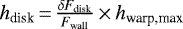 . This can be applied to the three systems with a dusty wall, resulting in hdisk = (0.46, 0.05, 0.12)R⋆ for Mon-660, 811, and 1308, respectively. These values can be compared to the model FWμ1.5 in Romanova et al. (2013), where the largest amplitude for the warp is 0.57 R⋆. For Mon-660, these values are comparable but for Mon-811 and Mon-1308, hdisk is lower. This means that for the last two cases, the interaction of the dipolar stellar magnetic field with the disk is weaker. Radiative MHD simulations are required to test these estimates using more detailed physical input.
For Mon-1140 Rsub,min > Rk is satisfied, such that there is no dust at Rk. This means that all the interpretation of the lightcurves is based on the bending wave. A value of δ = 0.01 for this system means that Fdisk need change by only 1% in order to explain the flux variability.
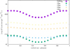 |
Fig. 4 Flux contributions in the optical and the IR for Mon-660 at i = 77°. The modeled CoRoT and 4.5 μm fluxes coming from the star are represented as filled squares and filled circles, respectively. The 4.5 μm fluxes coming from the wall and the disk are plotted with solid triangles and asterisks, respectively. The light asterisks represent the total modeled flux. |
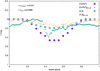 |
Fig. 5 Modeled optical and IR lightcurves for Mon-811 at i = 77°. The symbol definitions are the same as in Fig. 3. |
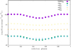 |
Fig. 6 Flux contributions in the optical and the IR for Mon-811 at i = 77°. The symbol definitions are the same as in Fig. 4. |
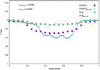 |
Fig. 7 Modeled optical and IR lightcurves for Mon-1140. The symbol definitions are the same as in Fig. 3. |
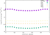 |
Fig. 8 Flux contributions in the optical and the IR for Mon-1140. The symbol definitions are the same as in Fig. 4. |
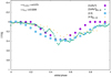 |
Fig. 9 Modeled optical and IR lightcurves for Mon-1308 at i = 77°. The symbol definitions are the same as in Fig. 3. |
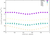 |
Fig. 10 Flux contributions in the optical and the IR for Mon-1308 at i = 77°. The symbol definitions are the same as in Fig. 4. |
5 Conclusions
Our main conclusion is that an optically thick wall at the keplerian radius associated to the periodicity of the observed lightcurve and an asymmetric disk are able to consistently explain the CoRoT and the Spitzer lightcurves of the NGC 2264 dippers Mon-660, Mon-811, Mon-1140, and Mon-1308. The stellar occultation by the wall or the asymmetrical structure in the disk is responsible for the modulation of the optical lightcurve and the emission from the partially occulted star, and the optically thick warp can explain the IR lightcurve.
A more detailed analysis of the effects of the distribution of material in the warp on the modeling will require us to run hydrodynamical simulations to get the distribution of gas and dust in the 3D structure. However, the simple structure considered here is enough to justify the basic picture to explain the lightcurves.
Acknowledgements
E.N. appreciates the support from the Institut de Planétologie et d’Astrophysique de Grenoble (Université Grenoble Alpes) during a sabbatical stay where most of the work was done. This project has received funding from the European Research Council (ERC) under the European Union’s Horizon 2020 research and innovation programme (grant agreement No 742095; SPIDI: Star-Planets-Inner Disk-Interactions).
Appendix A Degeneracy between i and hwarp,max
Values i and hwarp,max consistent with observed Δ[CoRoT] for each object.
There is a geometrical degeneracy between the parameters i and hwarp,max because a larger i means that a lower hwarp,max is required to get the amount of occultation necessary to explain the [CoRoT] lightcurve. In Table A.1 we put the pairs of values that produce the same amplitude for the observed Δ[CoRoT]. For each object, the i range is defined with the estimated value and its error obtained in the previous modeling of McGinnis et al. (2015). They obtained projected rotational velocities (v sin i) comparing Fibre Large Array Multi Element Spectrograph (FLAMES) or/and Hectochelle spectra to synthetic spectra and then they found i using the relation 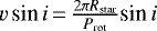 . The maximum value of i is fixed assuming a typical flared disk, such that the star is not completely occulted by the disk.
References
- Akeson, R. L., Walker, C. H., Wood, K., et al. 2005, ApJ, 622, 440 [NASA ADS] [CrossRef] [Google Scholar]
- Alencar, S. H. P., Teixeira, P. S., Guimarães, M. M., et al. 2010, A&A, 519, A88 [NASA ADS] [CrossRef] [EDP Sciences] [Google Scholar]
- Bouvier, J., Chelli, A., Allain, S., et al. 1999, A&A, 349, 619 [NASA ADS] [Google Scholar]
- Cody, A. M., Stauffer, J., Baglin, A., et al. 2014, AJ, 147, 82 [NASA ADS] [CrossRef] [Google Scholar]
- D’Alessio, P., Cantó, J., Calvet, N., et al. 1998, ApJ, 500, 411 [NASA ADS] [CrossRef] [Google Scholar]
- D’Alessio, P., Hartmann, L., Calvet, N., et al. 2005, ApJ, 621, 461 [NASA ADS] [CrossRef] [MathSciNet] [Google Scholar]
- D’Alessio, P., Calvet, N., Hartmann, L., et al. 2006, ApJ, 638, 314 [NASA ADS] [CrossRef] [Google Scholar]
- Debes, J. H., Poteet, C. A., Jang-Condell, H., et al. 2017, ApJ, 835, 205 [NASA ADS] [CrossRef] [Google Scholar]
- Flaherty, K., Muzerolle, J., Rieke, G., et al. 2012, ApJ, 748, 71 [NASA ADS] [CrossRef] [Google Scholar]
- Fonseca, N. N. J., Alencar, S. H. P., Bouvier, J., et al. 2014, A&A, 567, A39 [NASA ADS] [CrossRef] [EDP Sciences] [Google Scholar]
- Kesseli, A. Y., Petkova, M. A., Wood, K., et al. 2016, ApJ, 828, 42 [NASA ADS] [CrossRef] [Google Scholar]
- Kulkarni, A. K., & Romanova, M. M. 2013, MNRAS, 433, 3048 [NASA ADS] [CrossRef] [Google Scholar]
- Long, M., Romanova, M. M., & Lovelace, R. V. E. 2005, ApJ, 634, 1214 [NASA ADS] [CrossRef] [Google Scholar]
- Mathis, J. S., Rumpl, W., & Nordsieck, K. H. 1977, ApJ, 217, 425 [NASA ADS] [CrossRef] [Google Scholar]
- McClure, M. K., Calvet, N., Espaillat, C., et al. 2013, ApJ, 769, 73 [NASA ADS] [CrossRef] [Google Scholar]
- McGinnis, P. T., Alencar, S. H. P., Guimarães, M. M., et al. 2015, A&A, 577, A11 [NASA ADS] [CrossRef] [EDP Sciences] [Google Scholar]
- Morales-Calderón, M., Stauffer, J. R., Hillenbrand, L. A., et al. 2011, ApJ, 733, 50 [NASA ADS] [CrossRef] [Google Scholar]
- Nagel, E., D’Alessio, P., Calvet, N., et al. 2013, Rev. Mex. Astron. Astrofis., 49, 43 [NASA ADS] [Google Scholar]
- Pollack, J. B., Hollenbach, D., Beckwith, S., et al. 1994, ApJ, 421, 615 [NASA ADS] [CrossRef] [Google Scholar]
- Rice, T. S., Reipurth, B., Wolk, S. J., et al. 2015, AJ, 150, 132 [NASA ADS] [CrossRef] [Google Scholar]
- Romanova, M. M., Ustyugova, G. V., Koldoba, A. V., et al. 2013, MNRAS, 430, 699 [NASA ADS] [CrossRef] [Google Scholar]
- Romanova, M. M., Blinova, A. A., Ustyugova, G. V., et al. 2018, New Astron., 62, 94 [Google Scholar]
- Schneider, P. C., Manara, C. F., Facchini, S., et al. 2018, A&A, 614, A108 [NASA ADS] [CrossRef] [EDP Sciences] [Google Scholar]
- Scholz, A., Muzic, K., & Geers, V. 2015, MNRAS, 451, 26 [NASA ADS] [CrossRef] [Google Scholar]
- Stauffer, J., Cody, A. M., McGinnis, P., et al. 2015, AJ, 149, 130 [NASA ADS] [CrossRef] [Google Scholar]
- Stauffer, J., Cody, A. M., Rebull, L., et al. 2016, AJ, 151, 60 [NASA ADS] [CrossRef] [Google Scholar]
- Tannirkulam, A., Monnier, J. D., Millan-Gabet, R., et al. 2008, ApJ, 677, L51 [NASA ADS] [CrossRef] [Google Scholar]
- Terquem, C., & Papaloizou, J. C. B. 2000, A&A, 360, 1031 [NASA ADS] [Google Scholar]
- Venuti, L., Bouvier, J., Flaccomio, E., et al. 2014, A&A, 570, A82 [NASA ADS] [CrossRef] [EDP Sciences] [Google Scholar]
- Whitney, B. A., Robitaille, T. P., Bjorkman, J. E., et al. 2013, ApJS, 207, 30 [NASA ADS] [CrossRef] [Google Scholar]
All Tables
All Figures
|
Fig. 1 Sketch of the system modeled. The inclined straight lines represent two lines of sight with the same inclination crossing different sections of the system. The left line contributes to emission of the wall and the right line contributes to emission of the disk. In this case, all the stellar surface is occulted. |
| In the text | |
|
Fig. 2 Wall temperature (Twall in Kelvin) atthe vertical wall as a function of height (z in stellar radius) for Mon-660, Mon-811, and Mon-1308. |
| In the text | |
|
Fig. 3 Modeled optical and 4.5 μm lightcurves for Mon-660 at i = 77°. The modeled CoRoT lightcurve is represented by filled circles, and the modeled Spitzer photometric magnitudes at 4.5 μm are plotted as solid squares. For comparison the observed + 1σ CoRoT (points) and the + 1σ Spitzer 4.5 μm (asterixs) lightcurves are presented. We use all the cycles presented in McGinnis et al. (2015) to calculate the observed curves. At the upper left corner, we show the value for the mean standard deviation for the CoRoT and Spitzer data. |
| In the text | |
|
Fig. 4 Flux contributions in the optical and the IR for Mon-660 at i = 77°. The modeled CoRoT and 4.5 μm fluxes coming from the star are represented as filled squares and filled circles, respectively. The 4.5 μm fluxes coming from the wall and the disk are plotted with solid triangles and asterisks, respectively. The light asterisks represent the total modeled flux. |
| In the text | |
|
Fig. 5 Modeled optical and IR lightcurves for Mon-811 at i = 77°. The symbol definitions are the same as in Fig. 3. |
| In the text | |
|
Fig. 6 Flux contributions in the optical and the IR for Mon-811 at i = 77°. The symbol definitions are the same as in Fig. 4. |
| In the text | |
|
Fig. 7 Modeled optical and IR lightcurves for Mon-1140. The symbol definitions are the same as in Fig. 3. |
| In the text | |
|
Fig. 8 Flux contributions in the optical and the IR for Mon-1140. The symbol definitions are the same as in Fig. 4. |
| In the text | |
|
Fig. 9 Modeled optical and IR lightcurves for Mon-1308 at i = 77°. The symbol definitions are the same as in Fig. 3. |
| In the text | |
|
Fig. 10 Flux contributions in the optical and the IR for Mon-1308 at i = 77°. The symbol definitions are the same as in Fig. 4. |
| In the text | |
Current usage metrics show cumulative count of Article Views (full-text article views including HTML views, PDF and ePub downloads, according to the available data) and Abstracts Views on Vision4Press platform.
Data correspond to usage on the plateform after 2015. The current usage metrics is available 48-96 hours after online publication and is updated daily on week days.
Initial download of the metrics may take a while.