| Issue |
A&A
Volume 624, April 2019
|
|
|---|---|---|
| Article Number | A130 | |
| Number of page(s) | 8 | |
| Section | Astronomical instrumentation | |
| DOI | https://doi.org/10.1051/0004-6361/201935323 | |
| Published online | 25 April 2019 | |
Count-based imaging model for the Spectrometer/Telescope for Imaging X-rays (STIX) in Solar Orbiter
1
Dipartimento di Matematica, Università degli Studi di Genova, Via Dodecaneso 35, 16146 Genova, Italy
e-mail: This email address is being protected from spambots. You need JavaScript enabled to view it.
2
CNR-SPIN Genova, Via Dodecaneso 33, 16146 Genova, Italy
Received:
20
February
2019
Accepted:
13
March
2019
Abstract
The Spectrometer/Telescope for Imaging X-rays (STIX) will study solar flares across the hard X-ray window provided by the Solar Orbiter cluster. Similarly to the Reuven Ramaty High Energy Solar Spectroscopic Imager (RHESSI), STIX is a visibility-based imaging instrument that will require Fourier-based image reconstruction methods. However, in this paper we show that as for RHESSI, count-based imaging is also possible for STIX. Specifically, we introduce and illustrate a mathematical model that mimics the STIX data formation process as a projection from the incoming photon flux into a vector consisting of 120 count components. Then we test the reliability of expectation maximization for image reconstruction in the case of several simulated configurations that are typical of flare morphology.
Key words: techniques: image processing / instrumentation: detectors / methods: data analysis / Sun: X-rays / gamma rays / Sun: flares
© ESO 2019
1. Introduction
The Spectrometer/Telescope for Imaging X-rays (STIX; Benz et al. 2012) will be launched by the European Space Agency (ESA) as part of the Solar Orbiter (Müller & Marsden 2013) payload in order to provide a window on hard X-ray radiation that is emitted during solar flares in the energy range between a few and a few hundred keV. The main scientific goal of this instrument is to allow determining the timing, location, and spectrum of accelerated electrons by measuring the timing, location, and spectrum of their photon signature (Johns & Lin 1992; Holman et al. 2003; Piana et al. 2003, 2007; Brown et al. 2006; Kontar et al. 2011; Guo et al. 2012a,b, 2013; Torre et al. 2012; Huang et al. 2016; Dennis et al. 2018; Stackhouse & Kontar 2018). Specifically, STIX will convey the hard X-ray radiation from the Sun through 30 pairs of tungsten grids mounted at the extremity of an aluminum tube, and it will correspondingly record the signal using 30 cadmium-telluride detectors made of four rectangular pixels that are mounted behind each grid pair (Podgórski et al. 2013). A rigorous mathematical modeling of this signal formation process (Giordano et al. 2015) based on some numerical approximations showed that each system, consisting of two grids and a detector consisting of four pixels, provides a spatial Fourier component of the incoming flux, called visibility. Therefore, as in radio interferometry and in the case of the Reuven Ramaty High Energy Solar Spectroscopic Imager (RHESSI; Lin et al. 2002), the image reconstruction problem for STIX will be the inverse problem of inverting the Fourier transform of the photon flux from the limited data, which is represented by complex visibilities sampled in the spatial frequency domain, called the (u, v) plane (Hurford et al. 2002; Massone et al. 2009; Aschwanden et al. 2002; Duval-Poo et al. 2018; Felix et al. 2017; Sciacchitano et al. 2018). This imaging approach has some unquestionable advantages: for example, it may rely on a vast computational corpus of techniques developed in many different domains, and this type of algorithm may also exploit fast Fourier transform (FFT) to obtain reconstructions with a low computational burden. On the other hand, in the specific case of STIX, the sampling of the (u, v) plane is very sparse (only 30 visibilities are provided by the telescope, to be compared to the more than one hundred visibilities provided by a typical RHESSI observation), and therefore any imaging method has to make a significant effort in order to reduce the artifacts that may be induced by the undersampling of the frequency plane. Furthermore, as shown by Giordano et al. (2015), STIX visibilities are complex numbers whose real and imaginary parts are obtained by differences between count measurements: because the latter are Poisson data, visibility statistics is characterized by a lower signal-to-noise ratio (S/N) than the count statistics.
This paper contains two main results. The first is a mathematical model showing that count-based imaging is possible for STIX data. Specifically, the model builds up the matrix that reproduces the projection of the photon flux onto the count measurements recorded in each STIX pixel. The second result shows that a rather standard count-based imaging method, that is, expectation maximization (EM; Lucy 1974; Benvenuto et al. 2013), is able to reconstruct photon flux images with a reliability comparable to that provided by standard visibility-based methods (and to some extent even higher). The tests made in the paper use synthetic data corresponding to physically plausible configurations of flaring events that are produced by using the latest version of the STIX data processing software (DPS).
The paper is organized as follows. Section 2 introduces the count-based imaging model. Section 3 briefly reviews the count-based image reconstruction method. Section 4 shows the results of the image reconstruction procedure. Our conclusions are offered in Sect. 5.
2. Count-based imaging model
STIX consists of 30 pairs of grids, called subcollimators, that modulate the photon flux incident onto the telescope; in each subcollimator, the rear and the front grid have different orientations and pitches. Behind each subcollimator there is a cadmium-telluride detector that is vertically divided into four identical pixels. Photons passing through the grids produce typical Moiré patterns (Podgórski et al. 2013; Giordano et al. 2015) on the detectors, and are independently recorded by the pixels. Raw data measured by STIX are therefore 120 sets of photon counts. More precisely, Giordano et al. (2015) showed that the number of counts Aj, Bj, Cj, Dj recorded by the four pixels in the jth detector is approximated by
 (1)
(1)
 (2)
(2)
 (3)
(3)
and
 (4)
(4)
In these equations we have that
 (5)
(5)
 (6)
(6)
where l is the pixel width, h is the pixel height, L1 is the distance between the grids, L2 is the distance between the rear grid and the detector, S is the distance between Solar Orbiter and the Sun (here we assume S = 1 AU), and  and
and  are the wave vectors associated with the front and rear grid of detector j, respectively; and V(ξ) is the visibility sampled at (u, v) point ξ, that is,
 (7)
(7)
where ϕ(x) is the incoming flux. This definition and Eqs. (1)–(6) lead to
![Mathematical equation: $$ V({\boldsymbol{\xi }}_j) \simeq \frac{1}{4M_1} [(C_j - A_j) + i (D_j - B_j)] \exp \left(i\frac{\pi }{4}\right), $$](/articles/aa/full_html/2019/04/aa35323-19/aa35323-19-eq10.gif) (8)
(8)
which is the model for the visibility formation process in STIX. On the other hand, using in Eqs. (1)–(7) the fact that
 (9)
(9)
and some easy computation concerning complex numbers, we have
 (10)
(10)
 (11)
(11)
 (12)
(12)
and
 (13)
(13)
These latter four equations can be discretized in the Sun space, where ϕ(x) is defined, and this discretization leads to
 (14)
(14)
 (15)
(15)
 (16)
(16)
and
 (17)
(17)
where
 (18)
(18)
 (19)
(19)
 (20)
(20)
 (21)
(21)
Δx1 = 2X1/N1, Δx2 = 2X2/N2, and [ − X1, X1]×[−X2, X2] is the field of view (FOV); here we have assumed that the map center is (0, 0). Equations (14)–(21) prove that the link between the photon flux incident into the telescope and the number of counts recorded by its pixels can be modeled by means of the standard linear imaging equation
 (22)
(22)
where Φ ∈ ℝN1N2 is the discrete photon flux vector obtained by means of a lexicographical re-ordering of the N1 × N2 image to restore, c ∈ ℝ120 is the vector of counts recorded in the 4 pixels of all 30 detectors, and H ∈ ℝ120 × N1N2 is the matrix whose rows represent the transmission functions through the grid pair down to the detector pixels. In order to explicitly write the entries of this matrix in a more compact form, we observe that in Eq. (14),
 (23)
(23)
in Eq. (15),
 (24)
(24)
and in Eq. (17),
 (25)
(25)
We note that Eq. (16) is left untouched. Therefore the entries of H can be written as
![Mathematical equation: $$ H_{q,p} = \left[M_0 + 2 M_1\cos \left(2\pi \boldsymbol{\xi }_j \cdot \mathbf x _{p} + \frac{5 \pi }{4} -l\frac{\pi }{2} \right)\right]\Delta x_1 \Delta x_2, $$](/articles/aa/full_html/2019/04/aa35323-19/aa35323-19-eq28.gif) (26)
(26)
where q = (j, l), j = 1, …, 30 is the detector number, l = 1, …, 4 is the pixel number, p = 1, …, N1N2 and xp is the result of the reordering of xhk. Equations (22) and (26) represent the model for the count formation process in STIX. This model allows the use and formulation of image reconstruction methods that take as input the count vectors recorded by STIX pixels.
3. Expectation maximization
The use of the count-based framework set by Eqs. (22)–(26) instead of the visibility-based Fourier model of Eqs. (7) and (8) has two immediate advantages. The first is that in Eqs. (22) and (26) the data are more numerous because the counts are not mixed up (i.e., subtracted) in order to obtain visibilities, as in Eqs. (7) and (8). The second advantage is that the S/N in the problem defined by Eqs. (22)–(26) is higher than in Eqs. (7) and (8). Counts are Poisson variables, while visibilities are obtained by subtracting counts and therefore follow the Skellam statistics, in which the standard deviation is greater than the standard deviation associated with Poisson statistics. This is also shown empirically in Fig. 1: we have constructed the vector Φ corresponding to the Gaussian source in the left panel, and then we used the STIX DPS to randomly generate 50 vectors c. Using the components in c, we computed the corresponding 50 realizations of the 30 STIX visibilities. In the right panel of the figure, the S/N of each count component is compared to the S/N of the real and imaginary part of each visibility.
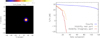 |
Fig. 1. Count statistics vs. visibility statistics in the case of 50 random realizations of the count vector produced by the STIX DPS. Left panel: simulated source configuration. Right panel: S/N associated with each data component. Specifically, the blue line represents the S/N of each count vector component, the orange line represents the S/N of the real part of each visibility, and the red line represents the S/N of the imaginary part of each visibility. The S/N values are ordered from the highest to lowest. |
Image reconstruction from STIX counts requires the numerical solution of Eq. (22), which is numerically instable owing to the conditioning of matrix H. However, a stable and reliable reconstruction can be obtained by stopping the EM iterative algorithm early. This algorithm exploits the Poisson nature of the noise affecting the components of vector c. The EM assumes that c is the realization of a random variable C with Poisson distribution so that the probability of observing c when the incoming flux is represented by Φ is
 (27)
(27)
The constrained maximum likelihood problem addresses the optimization problem
 (28)
(28)
where the positivity constraint is referred to each component of Φ. It can be proven that Eq. (28) can be expressed as a fixed-point problem, which can be solved by means of the successive approximation scheme
 (29)
(29)
where 1 is the vector with 1 for each component. The stopping rule introduced in Benvenuto & Piana (2014) provides an approximate solution of Eq. (22) in the sense of asymptotic regularization (Benvenuto 2017), which can realize a trade-off between numerical stability and data fitting.
4. Results
We tested EM on synthetic data simulated with the STIX DPS. We considered four configurations:
-
a double footpoint flare (configuration FF1) in which the sources have the same flux but different sizes;
-
a double footpoint flare (configuration FF2) in which the sources have the same flux and the same sizes;
-
a loop flare (configuration LF1) with large curvature;
-
a loop flare (configuration LF2) with small curvature.
For each configuration we performed three simulations, corresponding to three different levels of the incident photon flux: high statistics refers to an overall incident photon flux of 105 photons s−1 cm−2, medium statistics refers to an overall incident photon flux of 104 photons s−1 cm−2, and low statistics refers to an overall incident photon flux of 103 photons s−1 cm−2. Furthermore, for each configuration, we performed 10 random realizations of the count data vector. In all cases we assessed the reliability of the reconstructions by evaluating the morphology, the photometry, the spatial resolution, and the dynamic range provided by EM and compared these results with the ground truth and the results obtained by applying the most standard imaging algorithm implemented in the STIX DPS, that is, CLEAN, using visibilities as input. Figure 2 shows the reconstructions for the four configurations when the input data correspond to the medium statistics level. The complete set of results is described in Appendix. In order to provide a more quantitative comparison with the ground truth and CLEAN reconstructions, Table 1 contains the geometrical parameters associated with each original and reconstructed configuration together with the photometric parameters.
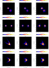 |
Fig. 2. Reconstructions of four source configurations characterized by an overall incident flux of 104 photons s−1 cm−2 (medium statistics). First column: simulated configurations (ground truth). Second column: count-based EM reconstructions. Third column: reconstructions provided by the visibility-based CLEAN algorithm. |
Reconstructions of four source configurations characterized by an overall incident photon flux of 104 photons cm−2 s−1 (medium statistics).
In order to assess the ability of the method to separate close sources, we simulated two identical circular Gaussian sources with a full width at half-maximum FWHM = 10 arcsec whose peaks gradually approach from 20 arcsec, through 14 arcsec, to 10 arcsec and made a spatial resolution analysis using EM and CLEAN. The results are presented in Fig. 3 for the three statistics levels. In most conditions, the two methods reproduce the locations of the sources rather well, but EM systematically performs better than CLEAN in estimating the peak intensity. When the peak distance in the original sources is 10 arcsec, EM can distinguish them at high statistics.
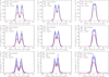 |
Fig. 3. Test on resolution power: two identical Gaussian functions with FWHM = 10 arcsec are moved closer and closer at 20 arcsec (left column), 14 arcsec (middle column), 10 arcsec (right column), reconstructed by EM and CLEAN and compared to ground truth. The results for all three statistics levels illustrate the reconstructed intensity profiles along the axis passing through the source centers, averaged over 10 random data realizations. The corresponding confidence strips are also reproduced. |
Figure 4 and Table 2 illustrate the results for the assessment of the ability of the methods to reproduce the dynamic range of two competing Gaussian sources. We again considered two circular Gaussian sources with the same size (FWHM = 10 arcsec), but with a brightness ratio (i.e., the ratio between the peak of the weakest source and the peak of the strongest source) b = 0.1, 0.3, 0.5. In this case, the locations are also reproduced rather well by both methods, and in this case, the peak intensities are also better estimated by EM. Neither method is reliable at all statistics when b = 0.1 to estimate the brightness ratio; furthermore, when b = 0.3 and b = 0.5 at low and medium statitstics levels, CLEAN produces slightly better results.
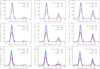 |
Fig. 4. Test on dynamic range: two Gaussian functions with brightness ratio b = 0.1 (left column), b = 0.3 (middle column), and b = 0.5 (right column) are reconstructed by EM and CLEAN, and the results are compared to ground truth. The results for all three statistics levels illustrate the intensity profiles along the axis passing through the source centers, averaged over 10 random data realizations. The corresponding confidence strips are also reproduced. |
Estimate of three brightness ratio values (b = 0.1, 0.3, 0.5) provided by EM and CLEAN for three statistics levels of the input photon flux.
5. Conclusions
We presented a model of image formation for STIX in which the incoming photon flux distribution was mathematically projected onto the counts recorded by the detector pixels. This model presents the advantages of a better S/N and of a higher number of input data at disposal for the reconstruction process than the ones that are available in the visibility-based model. Furthermore, this approach allows using EM as an imaging algorithm, and therefore allows exploiting the Poisson nature of the data statistic. The performances of EM show that the morphological parameters are reproduced with a level of detail that is comparable with the level provided by CLEAN. However, EM performs better photometrically, in line with the fact that this method has been explicitly conceived to maintain the overall count number during iterations. Interestingly, this good photometric behavior holds true even locally, as shown by the reconstructed values of the flux above the 50% level. Differently than CLEAN, EM simultaneously exploits both a positivity constraint and the conservation of flux at each iteration, and this probably explains its far better performances in spatial resolution power: EM is able to separate approaching sources very well (in Fig. 3 the ground truth falls in the confidence strip of the EM reconstructions for most conditions). CLEAN systematically underestimates the peak intensity of the reconstructed sources. However, at medium and high statistics levels for the incoming photon flux, CLEAN performs slightly better in reproducing the brightness ratio.
In conclusion, the count-based imaging model for STIX provides new image reconstruction capabilities for an imaging instrument that originally was designed for visibility-based approaches. Count-based methods can exploit the Poisson nature of data statistics in both Bayesian frameworks like EM and in deterministic settings that iteratively optimize the Kullbach–Leibler divergence (Bertero et al. 2010). On the other hand, visibility-based methods are typically rather fast because they can exploit FFT. The development of further statistical and deterministic regularization techniques to improve the count-based imaging model may be an interesting investigation theme for the next steps of the STIX imaging activity.
Acknowledgments
The authors kindly acknowledge Miguel Duval-Poo for useful discussions concerning the signal formation model.
References
- Aschwanden, M. J., Schmahl, E., & RHESSI Team. 2002, Sol. Phys., 210, 193 [NASA ADS] [CrossRef] [Google Scholar]
- Benvenuto, F. 2017, SIAM J. Numer. Anal., 55, 2187 [CrossRef] [Google Scholar]
- Benvenuto, F., & Piana, M. 2014, Inverse Prob., 30, 035012 [NASA ADS] [CrossRef] [Google Scholar]
- Benvenuto, F., Schwartz, R., Piana, M., & Massone, A. M. 2013, A&A, 555, A61 [NASA ADS] [CrossRef] [EDP Sciences] [Google Scholar]
- Benz, A. O., Krucker, S., Hurford, G. J., et al. 2012, Proc. SPIE, 8443, 84433L [CrossRef] [Google Scholar]
- Bertero, M., Boccacci, P., Talenti, G., Zanella, R., & Zanni, L. 2010, Inverse Prob., 26, 105004 [NASA ADS] [CrossRef] [Google Scholar]
- Brown, J. C., Emslie, A. G., Holman, G. D., et al. 2006, ApJ, 643, 523 [NASA ADS] [CrossRef] [Google Scholar]
- Dennis, B. R., Duval-Poo, M. A., Piana, M., et al. 2018, ApJ, 867, 82 [NASA ADS] [CrossRef] [Google Scholar]
- Duval-Poo, M. A., Piana, M., & Massone, A. M. 2018, A&A, 615, A59 [NASA ADS] [CrossRef] [EDP Sciences] [Google Scholar]
- Felix, S., Bolzern, R., & Battaglia, M. 2017, ApJ, 849, 10 [NASA ADS] [CrossRef] [Google Scholar]
- Giordano, S., Pinamonti, N., Piana, M., & Massone, A. M. 2015, SIAM J. Imag. Sci., 8, 1315 [CrossRef] [Google Scholar]
- Guo, J., Emslie, A. G., Kontar, E. P., et al. 2012a, A&A, 543, A53 [NASA ADS] [CrossRef] [EDP Sciences] [Google Scholar]
- Guo, J., Emslie, A. G., Massone, A. M., & Piana, M. 2012b, ApJ, 755, 32 [NASA ADS] [CrossRef] [Google Scholar]
- Guo, J., Emslie, A. G., & Piana, M. 2013, ApJ, 766, 28 [NASA ADS] [CrossRef] [Google Scholar]
- Holman, G. D., Sui, L., Schwartz, R. A., & Emslie, A. G. 2003, ApJ, 595, L97 [NASA ADS] [CrossRef] [Google Scholar]
- Huang, J., Kontar, E. P., Nakariakov, V. M., & Gao, G. 2016, ApJ, 831, 119 [NASA ADS] [CrossRef] [Google Scholar]
- Hurford, G. J., Schmahl, E. J., Schwartz, R. A., et al. 2002, Sol. Phys., 210, 61 [NASA ADS] [CrossRef] [Google Scholar]
- Johns, C. M., & Lin, R. P. 1992, Sol. Phys., 137, 121 [NASA ADS] [CrossRef] [Google Scholar]
- Kontar, E. P., Brown, J. C., Emslie, A. G., et al. 2011, Space Sci. Rev., 159, 301 [NASA ADS] [CrossRef] [Google Scholar]
- Lin, R. P., Dennis, B. R., Hurford, G. J., et al. 2002, Sol. Phys., 210, 3 [Google Scholar]
- Lucy, L. B. 1974, AJ, 79, 745 [NASA ADS] [CrossRef] [Google Scholar]
- Massone, A. M., Emslie, A. G., Hurford, G. J., et al. 2009, ApJ, 703, 2004 [NASA ADS] [CrossRef] [Google Scholar]
- Müller, D., Marsden, R. G., & St. Cyr, O. C., & Gilbert, H. R., 2013, Sol. Phys., 285, 25 [NASA ADS] [CrossRef] [Google Scholar]
- Piana, M., Massone, A. M., Kontar, E. P., et al. 2003, ApJ, 595, L127 [NASA ADS] [CrossRef] [Google Scholar]
- Piana, M., Massone, A. M., Hurford, G. J., et al. 2007, ApJ, 665, 846 [Google Scholar]
- Podgórski, P., Ścisłowski, D., Kowaliński, M., et al. 2013, in Proc. SPIE, 8903, 89031V [CrossRef] [Google Scholar]
- Sciacchitano, F., Sorrentino, A., Emslie, A. G., Massone, A. M., & Piana, M. 2018, ApJ, 862, 68 [NASA ADS] [CrossRef] [Google Scholar]
- Stackhouse, D. J., & Kontar, E. P. 2018, A&A, 612, A64 [NASA ADS] [CrossRef] [EDP Sciences] [Google Scholar]
- Torre, G., Pinamonti, N., Emslie, A. G., et al. 2012, ApJ, 751, 129 [NASA ADS] [CrossRef] [Google Scholar]
Appendix A: Additional material
The tables and figures in this Appendix describe the same analysis performed in Fig. 2 and in Table 1 but in the case of low and high statistics (Figs. A.1 and A.2, Tables A.1 and A.2).
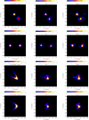 |
Fig. A.1. Reconstructions of four source configurations characterized by an overall incident photon flux of 103 photons cm−2 s−1 (low statistics). First column: simulated configurations (ground truth); second column: EM reconstructions; third column: reconstructions provided by the visibility-based CLEAN algorithm. |
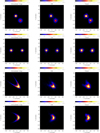 |
Fig. A.2. Reconstructions of four source configurations characterized by an overall incident photon flux of 105 photons cm−2 s−1 (high statistics). First column: simulated configurations (ground truth); second column: EM reconstructions; third column: reconstructions provided by the visibility-based CLEAN algorithm. |
Reconstructions of four source configurations characterized by an overall incident photon flux of 103 photons cm−2 s−1 (low statistics).
Reconstructions of four source configurations characterized by an overall incident photon flux of 105 photons cm−2 s−1 (high statistics).
All Tables
Reconstructions of four source configurations characterized by an overall incident photon flux of 104 photons cm−2 s−1 (medium statistics).
Estimate of three brightness ratio values (b = 0.1, 0.3, 0.5) provided by EM and CLEAN for three statistics levels of the input photon flux.
Reconstructions of four source configurations characterized by an overall incident photon flux of 103 photons cm−2 s−1 (low statistics).
Reconstructions of four source configurations characterized by an overall incident photon flux of 105 photons cm−2 s−1 (high statistics).
All Figures
|
Fig. 1. Count statistics vs. visibility statistics in the case of 50 random realizations of the count vector produced by the STIX DPS. Left panel: simulated source configuration. Right panel: S/N associated with each data component. Specifically, the blue line represents the S/N of each count vector component, the orange line represents the S/N of the real part of each visibility, and the red line represents the S/N of the imaginary part of each visibility. The S/N values are ordered from the highest to lowest. |
| In the text | |
|
Fig. 2. Reconstructions of four source configurations characterized by an overall incident flux of 104 photons s−1 cm−2 (medium statistics). First column: simulated configurations (ground truth). Second column: count-based EM reconstructions. Third column: reconstructions provided by the visibility-based CLEAN algorithm. |
| In the text | |
|
Fig. 3. Test on resolution power: two identical Gaussian functions with FWHM = 10 arcsec are moved closer and closer at 20 arcsec (left column), 14 arcsec (middle column), 10 arcsec (right column), reconstructed by EM and CLEAN and compared to ground truth. The results for all three statistics levels illustrate the reconstructed intensity profiles along the axis passing through the source centers, averaged over 10 random data realizations. The corresponding confidence strips are also reproduced. |
| In the text | |
|
Fig. 4. Test on dynamic range: two Gaussian functions with brightness ratio b = 0.1 (left column), b = 0.3 (middle column), and b = 0.5 (right column) are reconstructed by EM and CLEAN, and the results are compared to ground truth. The results for all three statistics levels illustrate the intensity profiles along the axis passing through the source centers, averaged over 10 random data realizations. The corresponding confidence strips are also reproduced. |
| In the text | |
|
Fig. A.1. Reconstructions of four source configurations characterized by an overall incident photon flux of 103 photons cm−2 s−1 (low statistics). First column: simulated configurations (ground truth); second column: EM reconstructions; third column: reconstructions provided by the visibility-based CLEAN algorithm. |
| In the text | |
|
Fig. A.2. Reconstructions of four source configurations characterized by an overall incident photon flux of 105 photons cm−2 s−1 (high statistics). First column: simulated configurations (ground truth); second column: EM reconstructions; third column: reconstructions provided by the visibility-based CLEAN algorithm. |
| In the text | |
Current usage metrics show cumulative count of Article Views (full-text article views including HTML views, PDF and ePub downloads, according to the available data) and Abstracts Views on Vision4Press platform.
Data correspond to usage on the plateform after 2015. The current usage metrics is available 48-96 hours after online publication and is updated daily on week days.
Initial download of the metrics may take a while.