| Issue |
A&A
Volume 668, December 2022
|
|
|---|---|---|
| Article Number | A145 | |
| Number of page(s) | 12 | |
| Section | The Sun and the Heliosphere | |
| DOI | https://doi.org/10.1051/0004-6361/202243907 | |
| Published online | 15 December 2022 | |
Forward fitting STIX visibilities
1
MIDA, Dipartimento di Matematica, Università degli Studi di Genova, Via Dodecaneso 35, 16146 Genova, Italy
e-mail: volpara@dima.unige.it, massone@dima.unige.it, piana@dima.unige.it
2
Department of Physics & Astronomy, Western Kentucky University, 1906 College Heights Blvd., Bowling Green, KY 42101, USA
3
Dipartimento di Scienze Matematiche “Giuseppe Luigi Lagrange”, Politecnico di Torino, Corso Duca degli Abruzzi, 24, 10129 Torino, Italy
4
CNR-SPIN, Via Dodecaneso 33, 16146 Genova, Italy
5
University of Applied Sciences and Arts Northwestern Switzerland, Bahnhofstrasse 6, 5210 Windisch, Switzerland
6
ETH Zürich, Rämistrasse 101, 8092 Zürich, Switzerland
7
Space Sciences Laboratory, University of California, 7 Gauss Way, 94720 Berkeley, USA
8
INAF – OATo, Strada Osservatorio 20, 10025 Pino Torinese, Torino, Italy
Received:
29
April
2022
Accepted:
17
October
2022
Aims. We seek to determine to what extent the problem of forward fitting visibilities measured by the Spectrometer/Telescope Imaging X-rays (STIX) on board Solar Orbiter becomes more challenging with respect to the same problem in the case of previous hard X-ray solar imaging missions. In addition, we aim to identify an effective optimization scheme for parametric imaging for STIX.
Methods. This paper introduces a global search optimization for forward-fitting STIX visibilities and compares its effectiveness with respect to the standard simplex-based optimization used so far for the analysis of visibilities measured by the Reuven Ramaty High Energy Solar Spectroscopic Imager (RHESSI). We made this comparison by considering experimental visibilities measured by both RHESSI and STIX, as weel as synthetic visibilities generated by accounting for the STIX signal formation model.
Results. We found that among the three global search algorithms for parametric imaging, particle swarm optimization (PSO) exhibits the best performances in terms of both stability and computational effectiveness. This method is as reliable as the simplex method in the case of RHESSI visibilities. However, PSO is significantly more robust when applied to STIX simulated and experimental visibilities.
Conclusions. A standard optimization based on local search of minima is not effective enough for forward-fitting the few visibilities sampled by STIX in the spatial frequency plane. Therefore, more sophisticated optimization schemes based on global search must be introduced for parametric imaging in the case of the Solar Orbiter X-ray telescope. The forward-fitting routine based on PSO proved to be significantly robust and reliable, and it could be considered as an effective candidate tool for parametric imaging in the STIX context.
Key words: Sun: flares / Sun: X-rays, gamma rays / techniques: image processing / telescopes
© The Authors 2022
 Open Access article, published by EDP Sciences, under the terms of the Creative Commons Attribution License (https://creativecommons.org/licenses/by/4.0), which permits unrestricted use, distribution, and reproduction in any medium, provided the original work is properly cited.
This article is published in open access under the Subscribe-to-Open model. Subscribe to A&A to support open access publication.
1. Introduction
Fourier imaging in astronomy was first introduced in radio astrophysics (Snell et al. 2019) and, indeed, interferometric arrays of on-Earth radio telescopes record sets of Fourier components of the incoming photon flux, which are referred to as “visibilities”. The first application of visibilities in space instruments probably dates back to around forty years ago during the Yohkoh mission (Kosugi et al. 1991). However, the first space instrument utilizing visibility-based imaging in an extensive and systematic way was designed by G. Hurford at the beginning of this century, with the NASA RHESSI mission for the hard X-ray observation of solar flares (Lin et al. 2002; Hurford et al. 2002). Nowadays, visibilities are the native form of measurements for the Spectrometer/Telescope for Imaging X-rays (STIX; Krucker et al. 2020), which is one of the remote sensing instruments on-board the ESA Solar Orbiter mission.
There are crucial differences between the processing of radio and hard X-ray visibilities. On the one hand, the dishes of radio telescopes are typically very large and hence collect very large numbers of photons (of the order of several thousands) characterized by very small energy per photon. On the other hand, RHESSI and STIX observe a much smaller number of photons characterized by much higher energies. For RHESSI, the Nyquist theorem and the requirement for an adequate sampling of a modulation cycle of its Rotating Modulation Collimators (Piana et al. 2022) imply that the number of independent visibilities available for imaging purposes is around 300 (however, statistically significant visibilities are often fewer, typically ranging between a few dozens and one hundred). For STIX, things are even worse: the sampled frequency points in this case are determined by the number and geometry of the sub-collimators, which are only 30.
Physical and geometrical constraints have significant impacts on the way visibilities are processed for image reconstruction. In the case of radio astronomy, interpolation in the visibility space and application of inverse Fourier transform are sufficient to obtain reliable images of the radio source (Arras et al. 2021). In the RHESSI and (even more) in the STIX frameworks, more sophisticated mathematics based on regularization theory for ill-posed problems is needed to reduce the ambiguity induced by such a sparse sampling of the data space (Massa et al. 2020, 2022; Perracchione et al. 2021; Massone et al. 2009).
Among visibility-based hard X-ray imaging methods, forward-fitting algorithms are aimed at estimating the input parameters of pre-defined shapes of the emitting sources by means of optimization procedures. The idea behind these algorithms is to model an emitting source by means of a parameterized function (typically obtained by modifications and replications of a 2D Gaussian function) and then to compute the parameter values that minimize the sum of the squared distance between the real and imaginary parts of the observed and predicted visibilities. The crucial tool for implementing these approaches is the optimization scheme applied in order to carry out such a minimization. Almost all forward-fitting-based RHESSI studies relied on simplex Nelder-Mead optimization, also known as AMOEBA Search (Press 2007; Aschwanden et al. 2002; Hurford et al. 2002), with results that are always reliable and robust (Xu et al. 2008; Kontar et al. 2011; Guo et al. 2012a,b, 2013; Dennis et al. 2018). (We note that the only exception to this simplex-based approach is probably represented by a study of the February 20, 2002 event where visibility forward-fitting is realized by means of a sequential Monte Carlo sampler; Sciacchitano et al. 2018).
Compared to non-parametric imaging methods, forward-fitting approaches have the advantage of directly providing estimates of the parameters of the X-ray sources (e.g., location, intensity, and dimension) and related uncertainties. Furthermore, details on the instrument response function can be more easily included in the forward-fitting process, thus increasing the accuracy and reliability of the results. On the other hand, parametric imaging methods have a major drawback in that the geometry of the retrieved X-ray configuration heavily depends on the a priori choice of number and shape of the parametric functions that are used for reconstructing the image. Hence, if the chosen parametric configuration does not reflect the actual morphology of the source, forward-fitting results could potentially be biased. However, as proved by comparisons with reconstructions obtained with non-parametric algorithms (see e.g., Piana et al. 2022; Massa et al. 2022), the parametric shapes that are adopted for modelling the X-ray sources usually represent a reliable approximation of the underlying flaring morphology.
The rationale of the present study was to assess whether simplex-based optimization is reliable as well in the case of STIX visibilities. The result of our analysis posits that when the number of available visibilities is as small as in the case of the ESA space telescope, there are significant experimental conditions where the use of AMOEBA for optimization provides an unreliable parameter estimation. We then proved that this drawback can be fixed by introducing parametric imaging strategies based on global optimization. In particular, our analysis suggests that the biology-inspired scheme (Kennedy & Eberhart 1995; Wahde 2008; Liu et al. 2011; Qasem & Shamsuddin 2011) – used for fitting STIX visibility amplitudes when fully calibrated visibilities were not yet available (Massa et al. 2021) – performs better than other global search schemes available in the literature. This optimization strategy is then applied for the first time to fully calibrated visibilities and its performances are compared with the ones of simplex optimization in the case of several data sets made of both synthetic and experimental STIX visibilities.
The plan of the paper is as follows. Section 2 provides a simple formalism illustrating the forward-fit problem for STIX. Section 3 compares some global search techniques for optimization problems and introduces the biology-inspired optimization algorithm. Section 4 contains the results of the analysis of both synthetic and observed STIX visibilities. Our comments and conclusions are offered in Sect. 5.
2. STIX forward-fit problem
The mathematical equation describing the image formation problem for STIX is

where the function ϕ = ϕ(x, y) represents the intensity of the X-ray photon flux originating from the (x, y) location on the Sun, V is the array containing the Nv complex values of the visibilities measured by STIX, and ℱ is the Fourier transform defined by

where  is the set of spatial frequencies sampled by the instrument. Therefore, the image reconstruction problem for STIX is the linear problem of determining the photon flux from a few experimental Fourier components. The STIX imaging problem in Eq. (1) and more generally, the image reconstruction problem from hard X-ray visibilities suffers from non-uniqueness of the solution (due to the limited (u, v) coverage of the telescopes) and from ill-conditioning. Hence, for overcoming these issues and determining a reliable solution of the imaging problem, several regularization methods have been implemented in the last decades. We refer the reader to Piana et al. (2022) for a recent review of hard X-ray imaging techniques developed so far.
In this paper we focus on forward fitting methods, whose goal is to provide estimates of the parameter values of parametric shapes used for modelling a flaring source. Physical considerations about hard X-rays emission and the experience gained during the RHESSI mission suggest that appropriate parametric shapes are those whose contour levels are shown in Fig. 1: a single Gaussian circular or elliptical source, a double Gaussian circular source and a loop source. A Gaussian circular source (circle henceforth) is a bi-dimensional isotropic Gaussian function described by the array of parameters (xc,yc,φ,w) representing the x and y coordinates of the center, the total flux, and the full width at half maximum (FWHM), respectively. Likewise, a Gaussian elliptical source (ellipse henceforth) consists of a bi-dimensional Gaussian function described by the array of parameters (xc,yc,φ,wM,wm,α) representing the x and y coordinates of the center, the total flux, the major and minor FWHM, and the orientation angle, respectively. A double Gaussian circular source (double henceforth) consists of the sum of two bi-dimensional isotropic Gaussian functions. In this configuration, the parameters to optimize are the same as in the circle for each source. Finally, a loop source (loop henceforth) consists of the replication of a number of circles (in this application we considered 11 circles) with centers located along a circumference. This configuration is described by the same parameters as for the ellipse with the addition of the loop angle β, that is the angle centered in the center of the circumference representing the curvature and subtended by the loop1. This shape is appropriate for modelling the thermal component of the emission and was not included in the PSO release used in Massa et al. (2021). The definition of loop shape we adopted is the same as the one implemented in the RHESSI forward-fit routine VIS_FWDFIT2 available in the Solar SoftWare (SSW) repository. A loop shape can be also obtained as a curved Gaussian ellipse, as done in previous works (see e.g., Aschwanden et al. 2002); however, determining which definition of loop configuration provides the most reliable and stable results is beyond the aim of this work and will be the subject of a future investigation.
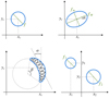 |
Fig. 1. Gaussian shapes considered in the parametric imaging process. Top left: Gaussian circular source (circle); top right: Gaussian elliptical source (ellipse); bottom left: replication of 11 circles (loop); bottom right: double Gaussian circular source (double). |
We use θ to denote the array of parameters characterizing each source shape. Then, forward-fitting STIX visibilities for parametric imaging requires the solution of the optimization problem:

where Θ is the parameter space and the target function χ2(θ) is defined as:
Nθ is the number of parameters of the source shape function ϕθ (either a circle, an ellipse, a double, or a loop) and σl is the uncertainty on the lth measured visibility amplitude.
The parametric imaging problem for STIX consists of selecting a specific shape function ϕθ as the candidate source, solving the problem in Eqs. (3) and (5) and using the corresponding source shape with the solution parameters for obtaining the reconstructed image. The computational core of this procedure is the optimization scheme applied for solving Eqs. (3) and (5). In the SSW repository, the VIS_FWDFIT routine utilizes the simplex scheme (AMOEBA) and was applied for the parametric imaging of all RHESSI data sets published so far and for the creation of the RHESSI image archive3. The effectiveness of this approach significantly decreases when the number of the available data becomes smaller, as in the case of STIX measurements. Therefore, in this framework, new optimization approaches must be introduced, which are able to avoid local minima by means of a more effective exploration of the parameter space.
3. From local to global optimization
Optimization problems can be described in terms of local or global optimization, where local optimization looks for the optimal solution just within a specific region of the search space, while global optimization explores the whole search space. As a consequence, local search algorithms are able to find global optima only if they are contained in the (limited) explored region, while global search algorithms are able to locate the global solution wherever it is, paying the price of a higher computational burden. The optimization scheme utilized in the VIS_FWDFIT routine (AMOEBA) belongs to the family of local search algorithms and relies on the Nelder-Mead algorithm (Avriel 2003). In order to overcome the AMOEBA limitations due to local search, here we applied approaches based on the application of global search techniques (Horst & Pardalos 2013). In particular, we considered Simulated annealing (Kirkpatrick et al. 1983), an evolutionary algorithm (Bäck 1996), and particle swarm optimization (PSO; Eberhart & Kennedy 1995). Simulated annealing implements a global search based on a probabilistic hill-climbing procedure inspired by statistical mechanics and mimics small thermodynamics fluctuations of a system of atoms starting from an initial configuration. The evolutionary algorithm, whereas, is inspired by the biological processes that allow population of individuals to adapt to the environment, assuming genetic inheritance and survival of the fittest individuals. Finally, PSO is another biology-inspired technique based on the model of intelligent cooperative behavior exhibited by certain animals such as flocks of birds or schools of fish.
In order to determine which global search algorithm better performs in the case of STIX parametric imaging, we implemented a numerical experiment exploiting STIX synthetic visibilities.
3.1. Comparison of global strategies
Synthetic STIX visibilities can be generated utilizing the STIX simulation software. Once a specific flare configuration is selected (e.g., circle, ellipse, double, loop), a Monte Carlo approach is used to reproduce the trajectory of the photon counts emitted from the source and measured by the detector pixels. Visibilities and related uncertainties are then computed from the simulated count measurements.
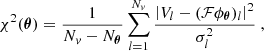
We considered three configurations mimicking non-thermal emissions (configurations C1, C2, C3, represented by two foot-points in different positions within the field of view and characterized by different dynamic ranges), and three configurations mimicking thermal emissions (configurations C4, C5, C6, represented by loop shapes in different position within the field of view and characterized by different orientation and loop angles). For each configuration, the three global search techniques have been applied to 25 random realizations of the corresponding STIX synthetic visibilities. The average values for the parameters characterizing each simulated configuration and the corresponding standard deviations are given in Table 1. The whole set of algorithms aptly reconstructs the expected values, with PSO offering more stable solutions, as suggested by systematically smaller standard deviation values. In the case of the reconstruction of configurations C1, C2, and C3, Simulated annealing requires an average computational time of 35.3 s, the evolutionary algorithm required 77.5 s and PSO required 8.2 s. This test has been performed on a Microsoft Windows 7 Enterprise (Intel(R) Core(TM) i7-2600 CPU at 3.40 GHz) machine. In the case of the reconstruction of configurations C4, C5, and C6, Simulated annealing required an average computational time of 18.3 s, the evolutionary algorithm required 72.6 s and PSO required 10.2 s. Furthermore, Fig. 2 shows an example of the kind of reconstruction (among the 25 ones) that has been most frequently provided by each method. In general, the three algorithms show a similar behavior, except for configuration C4, where PSO clearly demonstrates a better performance. Based on the results of this analysis, PSO will be used in the following as the global strategy to realize STIX parametric imaging.
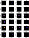 |
Fig. 2. Forward-fitting synthetic STIX visibilities associated with configurations mimicking three non-thermal and three thermal emissions, by means of Simulated annealing, evolutionary algorithm and PSO. First column: simulated configurations (the values of the configuration parameters are given in Table 1). Considering the 25 realizations of STIX visibility sets already used in Table 1, the second, third and fourth columns show the kind of reconstruction most frequently provided by Simulated annealing, evolutionary algorithm, and particle swarm optimization, respectively. |
3.2. Some details on PSO
Particle swarm optimization (PSO; Eberhart & Kennedy 1995) realizes optimization by mimicking swarm intelligence. The starting point of swarm intelligence is a random initialization of a set of points (candidate solutions) within the parameter space Θ, which gives rise to a swarm of particles or birds, with initial positions and velocities. Then, position and velocity of each bird are iteratively modified so that the swarm accumulates around the point of Θ corresponding to the minimum of the objective function (the χ2 function in the parametric STIX imaging). Specifically, at each iteration, the location of each particle is updated based on its velocity at the previous iteration (inertia), the best position visited by the particle since the beginning of the iterative process (individual cognition) and the global best position visited by the whole swarm (social learning). For details on the implementation of this procedure we refer the reader to Sect. 3 in Massa et al. (2021). The IDL PSO routine we have implemented and included in SSW is based on the implementation introduced by Mezura-Montes & Coello Coello (2011). Differently than for VIS_FWDFIT, the PSO-based approach (VIS_FWDFIT_PSO from now on) has been implemented in such a way that the user can decide which parameters have to be optimized, while keeping the other ones fixed. In both VIS_FWDFIT and VIS_FWDFIT_PSO implementations, the uncertainty on the parameters is estimated by generating a confidence strip around each parameter value: several realizations of the input data are computed by randomly perturbing the experimental set of visibility with Gaussian noise whose standard deviation is set equal to the errors on the measurements; for each realization, the optimization method is applied; and, finally, the standard deviation of each optimized source parameter is computed.
4. Numerical and experimental results
We compared the performances of VIS_FWDFIT_PSO to the ones of VIS_FWDFIT in the case of three experiments. First, we verified that PSO parameter estimates are comparable with the ones provided by AMOEBA in the case of RHESSI visibilities, when VIS_FWDFIT showed notable reliability and robustness. Then, we generated synthetic STIX visibilities from the six ground truth configurations considered in Sect. 3.1 and we applied VIS_FWDFIT_PSO and VIS_FWDFIT to these simulated data sets. Finally, we compared the robustness of the two optimization schemes with respect to different choices of the map center in the case of STIX experimental visibilities observed during the SOL2021-08-26T23:20 event.
4.1. RHESSI visibilities
On February 13, 2002, in the time range between 12:29:40 UT and 12:31:22 UT a flaring emission of class C1.3 showed a loop behavior in the thermal energy range between 6 and 12 keV. RHESSI well observed both such emission and on February 20 one week later, a C7.5 limb flare in the time range 11:06:05–11:07:42 UT characterized by a clearly visible non-thermal component in the energy range 22–50 keV. In Fig. 3 we show the reconstructions of these events provided by VIS_FWDFIT and VIS_FWDFIT_PSO. Specifically, for forward-fitting the visibilities observed during the February 13 event, we used a “loop” configuration; a “double” configuration was instead considered in the case of the February 20 event. To demonstrate that the source shapes adopted in the forward-fitting procedures are reasonable, we report in the third column of Fig. 3 the corresponding reconstructions obtained by means of the non-parametric method MEM_GE (Massa et al. 2020). Tables 2 and 3 contain the values of the parameters retrieved by VIS_FWDFIT and VIS_FWDFIT_PSO in the case of the February 13 and of the February 20 event, respectively.
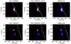 |
Fig. 3. Forward-fitting RHESSI visibilities with AMOEBA and PSO. Top row: reconstructions of the thermal component (6–12 keV) of the February 13, 2002 event 12:29:40–12:31:22 UT provided by VIS_FWDFIT (left), VIS_FWDFIT_PSO (middle) and MEM_GE (right). Bottom row: reconstruction of the non-thermal component (22–50 keV) of the February 20, 2002 event 11:06:05–11:07:42 UT. |
February 13, 2002 flare observed by RHESSI in the energy range 6–12 keV and in the time interval 12:29:40–12:31:22 UT.
February 20, 2002 flare observed by RHESSI in the energy range 22–50 keV and in the time interval 11:06:05–11:07:42 UT.
4.2. PSO and AMOEBA for STIX synthetic visibilities
We used the STIX simulation software to generate 25 new random realizations of synthetic visibility sets associated to the same six ground truth configurations considered in Sect. 3.1. We then applied VIS_FWDFIT and VIS_FWDFIT_PSO against these simulated sets and reported the corresponding results in Figs. 4 and 5. Specifically, in each figure the first row contains the ground truth configurations; the second and third rows contain examples of the kind of reconstructions that are most frequently provided by VIS_FWDFIT; and the fourth and fifth rows contain examples of the kind of reconstructions that are most frequently provided by VIS_FWDFIT_PSO. Table 4 contains the averaged values of the imaging parameters provided by the two routines, together with the corresponding standard deviations. Finally, the reduced χ2 values of the reconstruction in Figs. 4 and 5 are shown in Table 5.
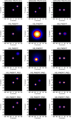 |
Fig. 4. Forward-fitting synthetic STIX visibilities associated with configurations mimicking three non-thermal emissions, by means of AMOEBA and PSO. First row: simulated configurations (the values of the configuration parameters are given in Table 4). Second and third rows: examples of the kind of reconstruction most frequently provided by VIS_FWDFIT. Fourth and fifth rows: examples of the kind of reconstruction most frequently provided by VIS_FWDFIT_PSO. |
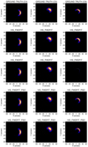 |
Fig. 5. Forward-fitting synthetic STIX visibilities associated with configurations mimicking three thermal emissions, by means of AMOEBA and PSO. First row: simulated configurations (the values of the configuration parameters are given in Table 4). Second and third rows: examples of the kind of reconstruction most frequently provided by VIS_FWDFIT. Fourth and fifth rows: examples of the kind of reconstruction most frequently provided by VIS_FWDFIT_PSO. |
4.3. PSO and AMOEBA for STIX experimental visibilities
On August 26, 2021 STIX observed a GOES C3 class flare close to the limb, whose light curves are represented in Fig. 6. We considered the data set corresponding to the time range between 23:18:00 and 23:20:00 UT and separately studied the thermal emission in the energy range between 6 and 10 keV and the non-thermal emission in the energy range between 15 and 25 keV. Furthermore, for this experiment, we did not use the six visibilities measured by the sub-collimators with finest resolution, since they are not yet fully calibrated. We first computed the discretized inverse Fourier transform of these visibilities by applying the back projection algorithm and we identified the location of the maximum of the reconstructed ‘dirty maps’ as reference map centers. We applied VIS_FWDFIT and VIS_FWDFIT_PSO to the visibility set corresponding to the thermal emission using the reference map center and we obtained the reconstructions represented in the first row of Fig. 7. Specifically, in these two panels, the level curves of the maps provided by VIS_FWDFIT and VIS_FWDFIT_PSO are manually superimposed on the EUV maps measured by SDO/AIA in the same time interval. Following the procedure described in Battaglia et al. (2021), the AIA maps were reprojected to make them appear as they would be seen from Solar Orbiter. In order to test the robustness of the PSO-based approach to a non-optimal choice of the map center, we then re-applied the two routines, but this time with the map center shifted by |Δx| = |Δy| = 10 arcsec. The results of this second experiment are provided in the two bottom rows of the same figure. Finally, we have repeated this experiment several times, for several values of the shift Δx in both directions, while keeping Δy fixed at Δy = 0. Just referring to the non-thermal regime reconstructions, in Table 6 we report the computed values for the FWHM of each source. We highlighted in red all cases where the relative variation of the FWHM is bigger than 10% with respect to the optimal case Δx = 0, for at least one source.
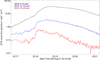 |
Fig. 6. Light curves for the August 26, 2021 event in the time range 23:16:46–23:21:14 UT. |
FWHM values associated to the two sources reconstructed in the parametric images of the August 26, 2021 event, non-thermal regime, by applying VIS_FWDFIT and VIS_FWDFIT_PSO to STIX visibilities for different map center values.
4.4. Analysis of the computational burden
As a final validation step, we analyzed the differences in the computational burden for the two schemes in the four cases involving the experimental RHESSI and STIX visibilities considered in this study. Specifically, Table 7 compares the computational costs needed by VIS_FWDFIT and VIS_FWDFIT_PSO both in the setting when the algorithms compute the uncertainties on the estimated parameters and in the setting when just one realization of the visibility set is considered. Tests have been performed on an Apple MacBook Pro M1 (Chip Apple M1, CPU 8-core, GPU 8-core) processor.
Computational time for VIS_FWDFIT and VIS_FWDFIT_PSO in the case of the four experimental data sets recorded by RHESSI and STIX during the events considered in the paper and summarized in the first column.
5. Comments and conclusions
The image reconstruction problem when data are hard X-ray visibilities is intrinsically linear and numerically unstable. Image reconstruction methods relying on regularization theory for ill-posed linear inverse problems have the advantage of providing reconstructions without any a priori assumption on the source morphology and typically via algorithms characterized by a relatively low computational burden. However, these linear approaches do not explicitly provide estimates of the imaging parameters. Parametric imaging relies on prior assumptions on the shape of the flaring source and often involves optimization schemes able to automatically provide estimates of the imaging parameters together with estimates of the corresponding statistical uncertainty.
This paper proved that AMOEBA, namely, the optimization scheme at the core of the SSW VIS_FWDFIT routine and which has shown a notable reliability for the forward fitting of RHESSI visibilities, sometimes produces unreliable results when applied to STIX visibilities. This is particularly evident in the tests presented in Figs. 4 and 5, where we used the same parametric configuration as the ground truth one for fitting the synthetic STIX visibilities. We are aware that in an operational setting, the actual flaring morphology is not a priori known; however, even under these simplified conditions, VIS_FWDFIT sometimes fails in reproducing the ground truth configuration (see e.g., configuration C2). The AMOEBA optimizer provides also unstable results when the center of the reconstructed map does not perfectly coincide with the centroid of the flaring morphology (see Fig. 7 and Table 6). For these reasons we have implemented and included in SSW a new forward fitting routine, namely, VIS_FWDFIT_PSO, in which the optimization step is performed by means of a biology-inspired algorithm, namely particle swarm optimization (PSO). This new routine has the same good performances with respect to VIS_FWDFIT in the case of RHESSI data, but is significantly more reliable in the case of STIX visibilities. Specifically, the new routine is more robust with respect to even slight modifications of the map center. The map-center location is currently estimated by performing a back-projection full-disk image and by determining the location of the most intense pixel. So, its uncertainty may depend on the back-projection pixel size and on the possible presence of sidelobes more intense than the back-projection core. In both cases we may have uncertainties larger than ∼4 arcsec (sometimes even much larger). The unreliable results provided by VIS_FWDFIT when the map-center is shifted from the reference location (i.e., the location of the peak of the back projection) are a reflection of the general instability of the method when applied to STIX visibilities. Increasing the accuracy in the estimate of the correct map-center would not be a solution for the VIS_FWDFIT misbehaviours, since the AMOEBA optimizer can get stuck in local minima even when the center of the map coincides with the center of mass of the flaring configuration (as shown in Figs. 4 and 5). The PSO optimizer is also able to provide satisfactory results with regard to the reconstruction of source configurations associated to the non-thermal regime, when the foot points are characterized by similar intensities. The misbehaviours, presented by VIS_FWDFIT when utilized against STIX visibilities, are probably due to the limited number of data available in this context (about one order of magnitude lower than those measured by RHESSI). Compared to the RHESSI case, the ambiguity of the solution of the image reconstruction is more pronounced in the STIX case and this is possibly reflected in a larger number of local minima in the objective χ2 function. As shown in Table 5, every time VIS_FWDFIT provides unreliable results, the associated χ2 value is larger than that of the corresponding (and reliable) VIS_FWDFIT_PSO reconstruction. This proves that the reason of the misbehaviours is in the AMOEBA optimizer getting stuck in the local minima. In contrast, the PSO optimizer is consistently able to reach the global minimum, thus demonstrating its superiority over AMOEBA in this context. The price to pay for this increased reliability is a heavier computational burden, which is more than one order of magnitude higher when the setting requires the computation of the uncertainties on the parameter estimates. However, this extra time is smaller with respect to other global search optimization schemes and is still very well within a reasonable time frame for data analysis in this context.
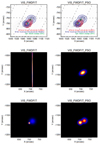 |
Fig. 7. Parametric images of the August 26, 2021 event obtained by applying VIS_FWDFIT (left column) and VIS_FWDFIT_PSO (right columns) on STIX observations. First row: contour level of the thermal (red) and non-thermal (blue) components superimposed onto the rotated AIA map (the 50% contour level of the AIA image is plotted in green). Second row: parametric images of the thermal component with the map-center shifted of |Δx|=|Δy| = 10 arcsec. Third row: same as the second row, but for the case of the non-thermal component. |
Finally, it may be possible to improve the performances of AMOEBA by finetuning the initialization of the parameters to be optimized. However, the changes to the initialization would be event-dependent and would require a priori information on the solution (e.g., an estimate of the location of the sources). In contrast, PSO is able to provide stable results without the need for an ad hoc initialization of the parameters, while only requiring as input a lower and upper bound for each parameter to be optimized.
Acknowledgments
Solar Orbiter is a space mission of international collaboration between ESA and NASA, operated by ESA. The STIX instrument is an international collaboration between Switzerland, Poland, France, Czech Republic, Germany, Austria, Ireland, and Italy. AFB and SK are supported by the Swiss National Science Foundation Grant 200021L_189180 and the grant ‘Activités Nationales Complémentaires dans le domaine spatial’ REF-1131-61001 for STIX. PM, EP, FB, AMM and MP acknowledge the financial contribution from the agreement ASI-INAF n.2018-16-HH.0. SG acknowledges the financial support from the “Accordo ASI/INAF Solar Orbiter: Supporto scientifico per la realizzazione degli strumenti Metis, SWA/DPU e STIX nelle Fasi D-E”.
References
- Arras, P., Reinecke, M., Westermann, R., & Enßin, T. A. 2021, A&A, 646, A58 [NASA ADS] [CrossRef] [EDP Sciences] [Google Scholar]
- Aschwanden, M. J., & Schmahl, E., & RHESSI Team 2002, Sol. Phys., 210, 193 [NASA ADS] [CrossRef] [Google Scholar]
- Avriel, M. 2003, Nonlinear Programming: Analysis and Methods (Chelmsford: Courier Corporation) [Google Scholar]
- Bäck, T. 1996, Evolutionary Algorithms in Theory and Practice: Evolution Strategies, Evolutionary Programming, Genetic Algorithms (New York: Oxford University Press) [CrossRef] [Google Scholar]
- Battaglia, A. F., Saqri, J., Massa, P., et al. 2021, A&A, 656, A4 [NASA ADS] [CrossRef] [EDP Sciences] [Google Scholar]
- Dennis, B. R., Duval-Poo, M. A., Piana, M., et al. 2018, ApJ, 867, 82 [NASA ADS] [CrossRef] [Google Scholar]
- Eberhart, R., & Kennedy, J. 1995, IEEE Int. Conf. Neural Netw., 4, 1942 [Google Scholar]
- Guo, J., Emslie, A. G., Kontar, E. P., et al. 2012a, A&A, 543, A53 [NASA ADS] [CrossRef] [EDP Sciences] [Google Scholar]
- Guo, J., Emslie, A. G., Massone, A. M., & Piana, M. 2012b, ApJ, 755, 32 [NASA ADS] [CrossRef] [Google Scholar]
- Guo, J., Emslie, A. G., & Piana, M. 2013, ApJ, 766, 28 [NASA ADS] [CrossRef] [Google Scholar]
- Horst, R., & Pardalos, P. M. 2013, Handbook of Global Optimization, (New York: Springer Science& Business Media), 2 [Google Scholar]
- Hurford, G., Schmahl, E., Schwartz, R., et al. 2002, Sol. Phys., 210, 61 [NASA ADS] [CrossRef] [Google Scholar]
- Kennedy, J., & Eberhart, R. 1995, Proceedings of ICNN’95-International Conference on Neural Networks (IEEE), 4, 1942 [CrossRef] [Google Scholar]
- Kirkpatrick, S., Gelatt, D., & Vecchi, M. 1983, Science, 220, 671 [CrossRef] [MathSciNet] [Google Scholar]
- Kontar, E. P., Hannah, I. G., & Bian, N. H. 2011, ApJ, 730, L22 [NASA ADS] [CrossRef] [Google Scholar]
- Kosugi, T., Murakami, T., & Sakao, T. 1991, Sol. Phys., 136, 17 [NASA ADS] [CrossRef] [Google Scholar]
- Krucker, S., Hurford, G. J., Grimm, O., et al. 2020, A&A, 642, A15 [NASA ADS] [CrossRef] [EDP Sciences] [Google Scholar]
- Lin, R. P., Dennis, B. R., Hurford, G. J., et al. 2002, Sol. Phys., 210, 3 [Google Scholar]
- Liu, Y., Ling, X., Shi, Z., et al. 2011, J. Softw., 6, 2449 [Google Scholar]
- Massa, P., Schwartz, R., Tolbert, A., et al. 2020, ApJ, 894, 46 [NASA ADS] [CrossRef] [Google Scholar]
- Massa, P., Perracchione, E., Garbarino, S., et al. 2021, A&A, 656, A25 [NASA ADS] [CrossRef] [EDP Sciences] [Google Scholar]
- Massa, P., Battaglia, A. F., Volpara, A., et al. 2022, Sol. Phys., 297, 93 [NASA ADS] [CrossRef] [Google Scholar]
- Massone, A. M., Emslie, A. G., Hurford, G. J., et al. 2009, ApJ, 703, 2004 [NASA ADS] [CrossRef] [Google Scholar]
- Mezura-Montes, E., & Coello Coello, C. A. 2011, SWEVO, 1, 173 [Google Scholar]
- Perracchione, E., Massa, P., Massone, A. M., & Piana, M. 2021, ApJ, 919, 133 [NASA ADS] [CrossRef] [Google Scholar]
- Piana, M., Emslie, A., Massone, A. M., & Dennis, B. R. 2022, Hard X-ray Imaging of Solar Flares (Berlin: Springer-Verlag) [CrossRef] [Google Scholar]
- Press, W. 2007, Numerical Recipes : the Art of Scientific Computing (Cambridge: Cambridge University Press) [Google Scholar]
- Qasem, S. N., & Shamsuddin, S. M. 2011, Appl. Softw. Comput., 1427 [Google Scholar]
- Sciacchitano, F., Sorrentino, A., Emslie, A. G., Massone, A. M., & Piana, M. 2018, ApJ, 862, 68 [NASA ADS] [CrossRef] [Google Scholar]
- Snell, R. L., Kurtz, S., & Marr, J. 2019, Fundamentals of Radio Astronomy: Astrophysics (Boca Raton: CRC Press) [CrossRef] [Google Scholar]
- Wahde, M. 2008, Biologically Inspired Optimization Methods: an Introduction (Boston: WIT Press) [Google Scholar]
- Xu, Y., Emslie, A. G., & Hurford, G. J. 2008, ApJ, 673, 576 [NASA ADS] [CrossRef] [Google Scholar]
All Tables
February 13, 2002 flare observed by RHESSI in the energy range 6–12 keV and in the time interval 12:29:40–12:31:22 UT.
February 20, 2002 flare observed by RHESSI in the energy range 22–50 keV and in the time interval 11:06:05–11:07:42 UT.
FWHM values associated to the two sources reconstructed in the parametric images of the August 26, 2021 event, non-thermal regime, by applying VIS_FWDFIT and VIS_FWDFIT_PSO to STIX visibilities for different map center values.
Computational time for VIS_FWDFIT and VIS_FWDFIT_PSO in the case of the four experimental data sets recorded by RHESSI and STIX during the events considered in the paper and summarized in the first column.
All Figures
|
Fig. 1. Gaussian shapes considered in the parametric imaging process. Top left: Gaussian circular source (circle); top right: Gaussian elliptical source (ellipse); bottom left: replication of 11 circles (loop); bottom right: double Gaussian circular source (double). |
| In the text | |
|
Fig. 2. Forward-fitting synthetic STIX visibilities associated with configurations mimicking three non-thermal and three thermal emissions, by means of Simulated annealing, evolutionary algorithm and PSO. First column: simulated configurations (the values of the configuration parameters are given in Table 1). Considering the 25 realizations of STIX visibility sets already used in Table 1, the second, third and fourth columns show the kind of reconstruction most frequently provided by Simulated annealing, evolutionary algorithm, and particle swarm optimization, respectively. |
| In the text | |
|
Fig. 3. Forward-fitting RHESSI visibilities with AMOEBA and PSO. Top row: reconstructions of the thermal component (6–12 keV) of the February 13, 2002 event 12:29:40–12:31:22 UT provided by VIS_FWDFIT (left), VIS_FWDFIT_PSO (middle) and MEM_GE (right). Bottom row: reconstruction of the non-thermal component (22–50 keV) of the February 20, 2002 event 11:06:05–11:07:42 UT. |
| In the text | |
|
Fig. 4. Forward-fitting synthetic STIX visibilities associated with configurations mimicking three non-thermal emissions, by means of AMOEBA and PSO. First row: simulated configurations (the values of the configuration parameters are given in Table 4). Second and third rows: examples of the kind of reconstruction most frequently provided by VIS_FWDFIT. Fourth and fifth rows: examples of the kind of reconstruction most frequently provided by VIS_FWDFIT_PSO. |
| In the text | |
|
Fig. 5. Forward-fitting synthetic STIX visibilities associated with configurations mimicking three thermal emissions, by means of AMOEBA and PSO. First row: simulated configurations (the values of the configuration parameters are given in Table 4). Second and third rows: examples of the kind of reconstruction most frequently provided by VIS_FWDFIT. Fourth and fifth rows: examples of the kind of reconstruction most frequently provided by VIS_FWDFIT_PSO. |
| In the text | |
|
Fig. 6. Light curves for the August 26, 2021 event in the time range 23:16:46–23:21:14 UT. |
| In the text | |
|
Fig. 7. Parametric images of the August 26, 2021 event obtained by applying VIS_FWDFIT (left column) and VIS_FWDFIT_PSO (right columns) on STIX observations. First row: contour level of the thermal (red) and non-thermal (blue) components superimposed onto the rotated AIA map (the 50% contour level of the AIA image is plotted in green). Second row: parametric images of the thermal component with the map-center shifted of |Δx|=|Δy| = 10 arcsec. Third row: same as the second row, but for the case of the non-thermal component. |
| In the text | |
Current usage metrics show cumulative count of Article Views (full-text article views including HTML views, PDF and ePub downloads, according to the available data) and Abstracts Views on Vision4Press platform.
Data correspond to usage on the plateform after 2015. The current usage metrics is available 48-96 hours after online publication and is updated daily on week days.
Initial download of the metrics may take a while.