| Issue |
A&A
Volume 624, April 2019
|
|
|---|---|---|
| Article Number | A124 | |
| Number of page(s) | 11 | |
| Section | Planets and planetary systems | |
| DOI | https://doi.org/10.1051/0004-6361/201935152 | |
| Published online | 24 April 2019 | |
Revisiting the cosmic-ray induced Venusian ionization with the Atmospheric Radiation Interaction Simulator (AtRIS)
1
Institut für Experimentelle and Angewandte Physik, Christian-Albrechts-Universität zu Kiel (CAU),
24118 Kiel, Germany
e-mail: This email address is being protected from spambots. You need JavaScript enabled to view it.
; This email address is being protected from spambots. You need JavaScript enabled to view it.
2
Jet Propulsion Laboratory, California Institute of Technology,
Pasadena,
CA, USA
Received:
29
January
2019
Accepted:
4
March
2019
Abstract
Context. Cosmic ray bombardment represents a major source of ionization in planetary atmospheres. The higher the energy of the primary cosmic ray particles, the deeper they can penetrate into the atmosphere. In addition, incident high energy cosmic ray particles induce extensive secondary particle cascades (“air showers”) that can contain up to several billion secondary particles per incoming primary particle. To quantify cosmic ray-induced effects on planetary atmospheres it is therefore important to accurately model the entire secondary particle cascade. This is particularly important in thick planetary atmospheres where the secondary particle cascades can develop extensively before being absorbed by the surface.
Aims. Inside the Venusian atmosphere, cosmic rays are the dominant driver for the ionization below an altitude of ~100 km. In this work we revisit the numerical modeling of the galactic and solar cosmic-ray induced atmospheric ionization for cosmic ray ions from Hydrogen (Z = 1) to Nickel (Z = 28) and investigate the influence of strong solar energetic particle events inside the Venusian atmosphere.
Methods. The Atmospheric Radiation Interaction Simulator (AtRIS), a newly developed simulation code to model the interaction of the near-(exo)planet particle and radiation field with the (exo)planetary atmosphere, was used to revisit the modeling of the altitude-dependent Venusian atmospheric ionization. Thereby, spherical geometry, the newest version of Geant4 (10.5) as well as the newest Geant4-based hadronic and electromagnetic interaction models were utilized.
Results. Based on our new model approach we show that previous studies may have underestimated the galactic cosmic ray-induced atmospheric ion pair production by, amongst others, underestimating the influence of galactic cosmic ray protons above 1 TeV/nuc. Furthermore, we study the influence of 71 exceptionally strong solar particle events that were measured as Ground Level Enhancements at the Earth’s surface, and show a detailed analysis of the impact of such strong events on the Venusian ionization.
Key words: Sun: activity / planets and satellites: terrestrial planets / planets and satellites: atmospheres
© ESO 2019
1 Introduction
In general, planetary atmospheres are exposed to a harsh radiation environment. Besides the stellar wind, ultraviolet, and X-ray radiation, in some cases we must take into account magnetospheric particle precipitation and cosmic rays (CR) of galactic or solar origin.
While solar energetic particles (SEPs) are accelerated in solar flares, coronal mass ejections or at interplanetary shocks (Reames 1999) galactic cosmic rays (GCRs) most likely are produced by diffusive shock acceleration at the shocks of supernova remnants (see, e.g., Hillas 2005; Büsching et al. 2005). Because of their different origins and acceleration mechanisms, therefore, the energy distribution of both components is slightly different: although exceeding the GCR flux by four orders of magnitude in the keV range, the SEP flux drops very rapidly at higher energies. Thereby particles with energies in the GeV range can only be observed in extreme SEP events, the so-called ground level enhancements (GLEs). In addition, the shape and the composition of the spectrum varies strongly from one event to another (Schmelz et al. 2012). GCRs on the other hand continuously impinge our heliosphere from all directions and can have energies well above the TeV range. However, due to the heliospheric magnetic field, which is frozen into the solar wind and thus reaches the outer heliospheric boundary, the flux of low-energy GCR particles is modulated with the changing solar activity.
Once inside the planetary atmosphere, CRs are the primary drivers of the planetary low-altitude atmospheric ionization. Thereby, the low energy CRs lose most of their energy by elastic collisions with atmospheric neutrals or ionization of the upper atmosphere before being stopped and absorbed. However, CRs with energies above ~1 GeV can induce extensive secondary particle cascades by undergoing inelastic scattering with atmospheric nuclei. Thereby, secondary mesons (π± and κ±), nucleons, gamma particles, and nuclear fragments are created, which may interact further. A sketch of the evolution of such a secondary particle cascade in the atmosphere is shown in Fig. 1. Once produced, secondary mesons almost immediately decay by producing muons, gamma particles as well as electrons. Thus, three branches develop within a cascade: the hadronic branch (neutrons, protons), the electromagnetic branch (electrons, positrons, and photons), and the muonic branch. Because the hadronic branch feeds the muonic and electromagnetic branches, it can also be seen as the core of the cascade, which is surrounded by a spreading secondary electromagnetic and muonic cone. As the atmospheric depth increases the cosmic ray cascade becomes increasingly evolved and the secondary particle flux continues torise until the so-called Pfotzer maximum (Pfotzer 1936) is reached. After this maximum, the average secondary particle energy is not sufficient enough to further drive the development of the particle cascade, and the cascade begins to die out. The Pfotzer maximum and the maximum altitude of the CR-induced ionization coincide. In the case of Earth, the Pfotzer maximum islocated at altitudes around 16–25 km. This value, however, strongly depends on the geomagnetic field strength, and thus the magnetic latitude (see, e.g., Herbst et al. 2013), as well as the solar activity (see, e.g., Bazilevskaya et al. 2008).
With a surface pressure almost 90 times higher, Venus has a much more massive atmosphere than its terrestrial sibling. Furthermore, since the Pioneer Venus Orbiter it is generally accepted that Venus has no significant global intrinsic magnetic field (Russell et al. 2012; Phillips & Russell 2012) that can act as a shield against low and high energy charged particles. Thus, the solar wind could, in principle, interact directly with the upper atmosphere. However, because UV radiation ionizes neutrals in the upper atmosphere, like on Earth, an ionosphere is generated. Currents arising from the interaction between the solar wind and the electrically conductive Venusian ionosphere lead to an induced magnetic field, and incoming solar wind particles areslowed down and diverted around the planet (see, e.g., Zhang et al. 2008). Because the induced magnetic field acts as an obstacle to the super-Alfvénic solar wind a Venusian bow shock, which only extents up to 0.4 Venusian radii from the surface, as well as a Venusian magnetosheath is generated (see, e.g., Russell et al. 1979; Svedhem et al. 2007). According to Taylor et al. (2018), this configuration is strong enough to minimize the erosion of the upper atmosphere by the solar wind. However, unlike the Earth’s magnetic field, the weak induced magnetic field can deflect charged energetic particles with energies only up to several hundreds of keV (see, e.g., Luhmann et al. 2004; Russell et al. 2006). Thus, similar to the Earth’s magnetic poles, most of the primary GCR particles have unrestricted access to the Venusian atmosphere. Moreover, recently, for example, Vech et al. (2015) investigated the influence of 42 strong interplanetary coronal mass ejections (CMEs), most of which accompanied by interplanetary shocks, on the Venusian environment. In agreement with Venus Express observationsa significant enhancement of the magnetic field strength within the magnetosheath due to these CMEs was found.
With a distance of only 0.7 AU from the Sun, Venus furthermore is exposed to higher particle fluxes from (strong) SEP events. Because Venus has a significantly more dense atmosphere, secondary particle showers will develop more extensively inside the Venusian atmosphere. However, unlike on Earth, only a small fraction of secondaries are able to reach and be absorbed by the Venusian surface. Since CRs are the main driver for the altitude-dependent atmospheric ion-electron pair production, the CR-induced ionization will have a strong influence on, for example, the atmospheric chemistry (see, e.g., Sinnhuber et al. 2018). Thus, it is necessary to quantify the effects of cosmic ray ionization and to understand its variability due to solar activity and sporadically induced strong SEP events.
The CR-induced ionization of the Venusian atmosphere has been investigated by, for example, Dubach et al. (1974), Borucki et al. (1982), Upadhyay et al. (1994) and Upadhyay & Singh (1995), who based their studies on approximations of the Boltzmanntransport equations. Only recently, Nordheim et al. (2015), Dartnell et al. (2015) and Plainaki et al. (2016) took modeling to a new level by applying a full 3D model approach based on the Monte Carlo toolkit Geant4 (see, e.g., Allison et al. 2016). Using the simulation code PLANETOCOSMICS (see, e.g., Desorgher et al. 2006) Nordheim et al. (2015) and Dartnell et al. (2015) describe the cosmic ray interactions and the production of the secondary particle cascades within the Venusian atmosphere, and were also the first to implement the contribution from protons, alpha particles and heavier ions (Z = 3–28). In addition, Plainaki et al. (2016) used the so called DYASTIMA tool (Paschalis et al. 2014) to investigate the Venusian atmospheric ionization due to both galactic and solar cosmic rays. They considered a SEP spectrum obtained from modeling of ground-based neutron monitor data (Plainaki et al. 2014), for the first time. Here we revisit the cosmic-ray induced ionization using the newly-developed Geant4-based Atmospheric Radiation Interaction Simulator (AtRIS, Banjac et al. 2019), a 3D simulation code developed to model the atmospheric ionization and radiation dose of exoplanets varying from hot Jupiters to Earth-like planets.
We show that the previously computed ion pair production rates are underestimated at altitudes above 100 km by a factor of two, as well as below 50 km by over one order of magnitude. Therefore, we investigate the influence of the hadronic interaction model used in the computations as well as the influence of the upper energy of the primary particle energy spectra. Furthermore, we investigate the influence of one of the strongest modern GLEs, strong SEP events that have been measured on the Earth’s surface, that occurred in October 1989. As we will show, primary Z > 1 particle spectra only have a minor influence on the SEP-induced atmospheric ionization. Thus, a more detailed study on the mean influence of such strong SEP events on the Venusian atmosphere, utilizing the proton spectra of 71 out of the 72 modern GLE events that occurred at Earth between 1942 and 2012 (see Raukunen et al. 2018), is presented. Besides, from historical records like the cosmogenic radionuclides, it is known that much stronger SEP events may also have occurred in the past. Thereby, of particular interest are two events: the Carrington event and the AD775 event (see also the study by Dartnell et al. 2015). Based on assumptions about the SEP event energy spectrum we will also investigate the influence of such strong events on the Venusian atmospheric ionization.
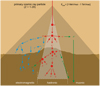 |
Fig. 1 Sketch of the altitude-dependent evolution of a secondary particle cascade induced by a high-energy primary cosmic ray particle (Z = 1–28). The cascade develops three branches: the electromagnetic branch mainly consisting of electrons, positrons and photons (also known as “soft component”), the muonic branch (the “hard component”), as well as the hadronic branch, mainly consisting of neutrons and protons (see, e.g., Bazilevskaya et al. 2008). |
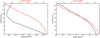 |
Fig. 2 Atmospheric profile based on the VIRA model (see Keating et al. 1985; Seiff et al. 1985) used in this study. Left panel: altitude-dependent temperature (black line) and density profile (red line). Right panel: corresponding atmospheric depth (black line) and pressure profiles (red line). |
2 The Atmospheric Radiation Interaction Simulator (AtRIS)
AtRIS, a Geant4-based (Monte Carlo) particle transport code, has recently been developed by Banjac et al. (2019) in order to simulate thepropagation of energetic particles through (exo)planetary atmospheres and regolith. Thereby, AtRIS allows for rather flexible geometry and composition definitions of the planet. As particular input, the user has to define an interface forthe planetary atmospheric model. By now interfaces for the NRLMSISE-00 (Picone et al. 2002) model (Earth) andthe Mars Climate Database (MCD, see Forget et al. 2006) exist. Similarly, we then implemented an interface for the Venus International Reference Atmosphere (VIRA, see, e.g., Kliore et al. 1992) day-side model.
AtRIS can calculate ion and electron pair production rates, secondary particle distributions (as a function of, e.g., energy, directionality, altitude), as well as absorbed and equivalent dose rates. While AtRIS does not provide the tracking of charged particles through a magnetic field, the user is given full control over the specification of the primary particle flux. Similarly, control over hadronic and electromagnetic processes is provided via the standard Geant4 message and compounded physics list naming scheme (Allison et al. 2016; Geant4 Collaboration 2018).
The main features of AtRIS are (i) the Planet Specification Format, (ii) the Atmospheric Response Matrices (ARMs), quantifying the relationship between primary energy and altitude-dependent ionization as well as equivalent/absorbed dose rate, and finally, (iii) the spectrum folding procedure used to calculate net quantities like the electron-ion pair production rate, by implementing a convolution of a measured spectrum and the ARM. A more detailed description can be found in Banjac et al. (2019). So far AtRIS has successfully been validated for the terrestrial and Martian atmosphere (see Banjac et al. 2019; Guo et al. 2019).
3 The simulation setup
As proposed by Plainaki et al. (2016) here the Venusian environment is modeled for spherical geometry. Thereby, AtRIS was configured as follows: a core with a radius comparable to the average Venusian radius (6052 km) was used, a soil composition of approximately as 50% Si, 40% O, and 10% Fe (mass fractions) was assumed, and the crust (soil) sheet was set to a thickness of 100 m. The upper limit of the Venusian atmosphere was set at 150 km and divided into 500 m thick layers. The total shielding thickness of the Venusian atmosphere is on the order of 105 g cm−2 (Borucki et al. 1982), which is almost two orders of magnitude higher compared to Earth (~ 1033 g/cm−2). Therefore, only negligible secondary particle production, and thus ionization, is expected at the Venusian surface.
To be able to compare our results with the most recent model efforts directly we have used the same atmosphere, source altitude and input spectrum as in the studies by Nordheim et al. (2015), Dartnell et al. (2015) and Plainaki et al. (2016). Thus, the atmospheric setup of our studies is based on VIRA (see Kliore et al. 1992) that utilizes the day-side atmospheric parameter set by Seiff et al. (1985) at low to mid-atmospheric layers (surface to 100 km) for low latitudes (ϕ < 30°) and those proposed by Keating et al. (1985) for altitudes up to 150 km at low latitudes (ϕ < 16°). Moreover, an atmospheric composition of 96.5% CO2 and 3.5% N2 has been applied. The corresponding temperature, density, and pressure profiles are displayed in the panels of Fig. 2.
In order to simulate hadronic and electromagnetic interactions, and thus the evolution of secondary particle cascades, inside an atmosphere, the Geant4 toolkit provides several packages (physics lists) a user can choose from. While Nordheim et al. (2015) and Dartnell et al. (2015) base their studies on the QGSP_BIC_HP model we have like Plainaki et al. (2016) used the more advanced FTFP_BERT_HP model. While the QGSP_BIC_HP as well as the QGSP_BERT_HP (see Sec. 4.1.2) models use the Quark-Gluon-String (QGS) model for high energy particle interactions different cascade models are applied for particle energies below 10 GeV. The FTFP_BERT_HP model, however, is explicitly recommended for high energy particle physics, and thus radiation protection and shielding applications. Our computations are based on the Bertini-style cascade for hadrons with energies below 5 GeV as well as the Fritiof (FTF) model (see, e.g., Nilsson-Almqvist & Stenlund 1987) for particle interactions of mesons, nucleons and hyperons with energies between 3 and 100 TeV. Furthermore, the standard em constructor (see, e.g., Allison et al. 2016) has been used for the electromagnetic interactions.
As input for the time-dependent GCR flux at the top of the Venusian atmosphere, such as Nordheim et al. (2015), Dartnell et al. (2015), and Plainaki et al. (2016), we used the CREME2009 model1 (see, e.g. Tylka et al. 1997). This model provides the differential intensities for all particles from protons to nickel in an energy range of 1 MeV nuc−1 up to 100 GeV nuc−1 at 1 AU. Because the solar magnetic field modulates GCRs, their flux shows an anticorrelation to the solar activity. In this study, we have investigated the atmospheric ionization for the solar minimum as well as maximum conditions in which solar energetic particle events were absent. As suggested by Nordheim et al. (2015) the high energy tail of the particle fluxes up to 1 TeV nuc−1 was extended by applying an element-dependent power law. Although the Venusian orbit is about 30% closer to the Sun than that of Earth a re-scaling of the 1 AU GCR flux model is not necessary because the radial gradients of GCR particles in the inner solar system are small (see, e.g., Heber et al. 1996; Morales-Olivares & Caballero-Lopez 2010; Gieseler & Heber 2016).
Furthermore, the CREME2009 model also provides the Z = 1–28 spectra for particularly strong SEP events. Being accelerated at shock fronts of solar flares and CMEs, SEP spectra typically show energies up to hundreds of MeV and reach planets anisotropically. To investigate the influence of ordinary strong solar events on the Venusian atmosphere the SEP spectra of the October 1989 event were extracted from the CREME2009 model. However, because the flux of SEP events strongly depends on the orbital distance a 1/R2 scaling has been applied to the spectra. To study the influence of strong solar energetic particles on the Venusian atmosphericionization even further, we used the proton fluence spectra of 71 GLE events measured during the neutron monitor era (Raukunen et al. 2018), of which the strongest one occurred on February 23, 1956 (hard spectrum, GLE05). However, from observations of a particularly strong solar white-light flare on September 1, 1859 that was followed by the so-called Carrington-event, and from cosmogenic radionuclide records of the past ~10 000 yr, that show strong increases of over 15% above the production background around, for example, around AD775 (see, e.g., Miyake et al. 2012; Mekhaldi et al. 2015), we now know that even stronger events occurred throughout the Sun’s history. Model studies of the terrestrial cosmogenic radionuclideproduction showed that the event of AD775 was well over one order of magnitude stronger then GLE05 (see, e.g., Kovaltsov & Usoskin 2014; Herbst et al. 2015). The influence of the two historical events will also be modeled in this study.
4 Results and discussion
Based on the atmospheric response matrices (ARMs) the total altitude-dependent atmospheric ionization is computed. Thereby, the modeled ion pair production rates strongly depend on the atmospheric density as well as the mean atmospheric ionization potential w. For the Venusian atmosphere most often a value of 33.5 eV is assumed in order to produce one ion-electron pair in a CO2 -dominated atmosphere (see Borucki et al. 1982). However, the numerical studies by Simon Wedlund et al. (2011) suggest that the currently used w-values may not be as accurate. For CO2 -dominated atmospheres they propose a w-value of 28.7 ± 4.3 eV, which is slightly lower than the values reported by previous theoretical and experimental studies (see, e.g., Fox et al. 2008; ICRU 1993, respectively). In order to compare our model results with previously published efforts in this study we use the “traditional” value of 33.5 eV. However, as already mentioned in Nordheim et al. (2015) re-scaling the presented ionization profiles is rather easy: dividing the presented values by a mean of 1.17 will result in values corresponding to an atmospheric ionization potential as suggested by Simon Wedlund et al. (2011).
4.1 Galactic cosmic ray-induced ionization
The upper left panel of Fig. 3 shows a comparison of the modeled terrestrial (blue line) and Venusian (red line) altitude-dependent total ion pair production rate (taking into account particles with Z = 1–28) during solar minimum conditions. As can be seen, the Pfotzer maximum, the maximum of the secondary particle cascade evolution, and thus the ionization maximum on both planets is reached at quite different altitudes: while known to occur around 16–20 km at Earth, the maximum is predicted to occur at altitudes between 62 and 64 km in the Venusian atmosphere. As expected, due to the much higher total shielding thickness of the Venusian atmosphere, the ion pair production rate at the Venusian surface is also much lower than at the Earths surface. We note, that the following panels will solely focus on the results for the Venusian atmosphere. The upper right panel shows a comparison of the altitude-dependent total ion pair production rates as function of the used Venusian ionization potential w. While the solid red line corresponds to w = 33.5 eV the dashed line and its error band represent values based on the ionization potential proposed by Simon Wedlund et al. (2011).
The lower left panel of Fig. 3 shows the contribution of Z = 1 (protons, dashed lines) and Z = 2–28 (dotted lines) particles to the total atmospheric ionization during solar minimum conditions. Here the results by Nordheim et al. (2015, black lines) are compared with our results (red lines). As can be seen, protons (Z = 1) have a much higher influence on the atmospheric ionization than all other particles combined. But the contributionof the latter (in particular that of C, N, O, Si, and Fe) can not be neglected. Furthermore, although being in good agreement with each other at mid-altitudes (100–40 km) at altitudes above ~120 km, our values are more than five times higher than those modeled by Nordheim et al. (2015). However, looking at the ionization at lower altitudes reveals a different picture. Here, the ion-pair production proposed by Nordheim et al. (2015) is roughly twice as high as that modeled in this study. In addition, the influence of the solar activity on the Venusian ionization is shown in the lower right panel. Here our modeled production rate values (in red) and those modeled by Plainaki et al. (2016; in blue) are given for both solar minimum (solid lines) and solar maximum (dashed lines) conditions. As can be seen, the solar activity has only a slight influence on the altitude of the production rate maximum. Both studies show a decrease in the ion-pair production rate at altitudes above 80 km during strong solar activity in the order of ~40%. However, although they are based on the same hadronic interaction model, strong differences between the models occur at lower altitudes. As will be discussed in the following, these differences are caused by the underlying simulation-dependent statistics.
In addition, the results by Dubach et al. (1974; gray), Borucki et al. (1982; blue) and Upadhyay & Singh (1995; green) are shown. Since the latter model efforts only cover certain altitude ranges a full altitude-dependent comparison is not possible. Nevertheless, the model-dependent ion-pair production rate values, as well as the corresponding altitudes of the ionization maximum, are given in Table 1. It becomes evident that the production rate values by Upadhyay & Singh (1995) are about two order of magnitude higher than the results of all other studies and show a second ionization peak at an altitude around 25 km due to the influence of muons, a feature which could not be confirmed by the three full 3D model results. The predicted ion-pair production rate values at this altitude are more than six orders magnitude higher than the values computed with AtRIS.
Aplin (2006) estimate a near-surface ion pair production rate of 0.01 ion pairs (cm3 s)−1 due to radioactive decay. Comparing the various studies Borucki et al. (1982) predicts a cosmic ray ionization rate that is comparable to that due to radioactive decay. However, our new results show that the predicted near-surface ionization rates due to radioactive decay is roughly one order of magnitude higher than those due to the influence of cosmic rays. In other words, radioactive decay dominates over cosmic ray ionization at the Venusian surface.
In the following, the differences between the full 3D model attempts are studied in more detail. Potential causes for such differences are: (a) the use of different Geant4 versions (9.4, 10.1 and 10.5), (b) the use of different hadronic interaction models (QGSP_BIC_HP vs. FTFP_BERT_HP), as well as (c) the upper energy limit of the Z = 1–28 GCR particle fluxes.
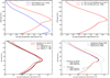 |
Fig. 3 Upper left panel: altitude-dependent total ion pair production rates during solar minimum conditions at Venus (thisstudy, red solid line) and at Earth (blue line, see Banjac et al. 2019) as a reference. The following panels only address the Venusian ionization. Upper right panel: influence of the applied ionization potential w. Shown here are the model results for the w-values by Borucki et al. (1982, w = 33.5 eV, red solid line) and Simon Wedlund et al. (2011, w = 28.7 ± 4.3 eV, red dashed line and corresponding error band). Lower left panel: contribution of Z = 1 (protons, dashed lines) and Z = 2–28 (dotted lines) particles to the total atmospheric ionization (solid line) during solar minimum conditions. The results by Nordheim et al. (2015, black curves) are compared to the results of this study (red curves). Lower right panel: comparison of the altitude-dependent ionization rates by Plainaki et al. (2016, light blue curves) and the results of our study during solar minimum (solid lines) and solar maximum (dashed lines) conditions. In addition the results by Dubach et al. (1974; blue), Borucki et al. (1982, orange), and Upadhyay & Singh (1995; purple) are displayed. |
Estimates of the altitude hmax (km) and the ion pair production rate Q of the Venusian Pfotzer maximum during solar minimum (solar maximum) conditions modeled by Dubach et al. (1974, DU74), Borucki et al. (1982, BO82), Upadhyay & Singh (1995, US95), Nordheim et al. (2015, NO15), Plainaki et al. (2016, PL16) and this work (HE19).
4.1.1 Influence of the used Geant4-version
Since the publications by Nordheim et al. (2015), Dartnell et al. (2015), and Plainaki et al. (2016), multiple updates of the Geant4 codehave been released. Although not stated in the literature, the three previous full 3D model efforts most likely were based on Geant4 9.4 and 10.1, respectively. In our model setup, however, we use the (up to now) newest Geant4 version (10.5), which has been published in December 2018. Since Geant4 9.4, significant changes on the physics lists as well as the hadronic and electromagnetic physics have been introduced. In case of hadronic physics since Geant4 9.4, for example, (a) the fragmentation part of the QGS model has been improved significantly, which results in wider and longer hadronic showers as well as lower energy responses, (b) the evaporation spectrum of the Bertini-like intra-nuclear cascade model (BERT) has been improved, which reduced the overproduction of low-energy neutrons and protons, as well as (c) new updates of the FTF and QGS string models have been released in the latest version2.
4.1.2 Influence of the different hadronic interaction models
In order to study the influence of different hadronic interaction models on the modeled Venusian ionization profile we computed the altitude-dependent GCR proton-induced ion-pair production rate values based on four different hadronic models: the QGSP_BIC model, the QGSP_BIC_HP model (as used by Nordheim et al. 2015), the FTFP_BERT model as well as the FTFP_BERT_HP model (as used by Plainaki et al. 2016, and in this study). As can be seen in the upper panel of Fig. 4 differences between themodels, in particular, can be found at high altitudes (above 120 km), at the ionization maximum (~67 km), as well as the near-surface region (up to 10 km). At high altitudes, the simulations based on the FTFP_BERT_HP model (red curve) show ionization rates that are more than one order of magnitude higher than, for example, those based on the QGSP_BIC model (light blue curve). Also shown are the results of Nordheim et al. (2015, black dashed line). A comparison to our computations based on the QGSP_BIC_HP model (black solid line) shows differences at low and high altitudes. These most likely can be explained by the changes to the Geant4 hadronic physics, as described above. The same is also true for the differences between the results by Plainaki et al. (2016) and our computations based on the FTFP_BERT_HP model (see, e.g., lower right panel of Fig. 3).
4.1.3 Influence of the upper energy limits
However, another crucial factor is the upper energy limit of the GCR spectrum. The middle panel of Fig. 4 shows the modeledproton-induced ion-pair production rate values based on three different spectral energy ranges: from 1 MeV up to 100 GeV (blue), from 1 MeV up to 1 TeV (red) and, for the first time, from 1 MeV up to 10 TeV (orange) using the same power law extrapolation as previously discussed for the 1 MeV to 1 TeV spectrum. As can be seen, the ionization rates by Nordheim et al. (2015, black dotted line) and Plainaki et al. (2016, light blue line) are in good agreement to our computations based on primary particle energies in the energy range between 1 MeV up to 1 TeV at altitudes above ~30 km. However, while the results by Nordheim et al. (2015) may overestimate our modeled surface production rates by a factor of two the results by Plainaki et al. (2016) strongly underestimate the other modeled production rate values below an altitude of 30 km. As discussed in Plainaki et al. (2016) their model approach is less reliable at large atmospheric depths and, thus, their model results for the low-altitude Venusian atmosphere should be treated with caution.
However, as shown here for the first time, the fact that primary protons in the energy range of 1–10 TeV cannot be neglected when it comes to investigating the Venusian atmospheric ionization is of much more interest. It shows that these high-energetic primaries induce additional ion-pair production at all altitudes below the ionization maximum. For a more detailed study, the lower panel of Fig. 4 shows the influence of primary particles on the Venusian ion pair production below an altitude of 60 km. Therefore, protons within selected energy bins are displayed, for example, 100–158 GeV (in blue), 1–1.564 TeV (in red) as well as 6.309–10 TeV (in orange). As can be seen, primary particles within 1 MeV up to 100 GeV are the dominant source for the ion pair production above ~40 km while protons with energies between 100 GeV and 1 TeV are the main motor for the ionization between 40 and 20 km. However, the atmospheric ionization below ~10 km is dominated by the influence of primary particles (and their induced secondary particle cascades) with even higher energies. As can be seen the maximum production can be attributed to protons with energies between 2.5 and 6.3 TeV. Thus, primary protons up to at least 6 TeV need to be taken into account in order to describe the Venusian ion pair production as precisely as possible. We note that for protons with energies above 6 TeV the energy content of the flux at these altitudes becomes smaller. Nevertheless, 10 TeV protons account for up to 10% of the surface ionization.
The reliability of the different computation methods depends on the reliability of the underlying statistics. The uncertainties of our model results are on the order of 5% of which about 3% account for the uncertainties of the atmospheric model. This, however, is negligible in view of the uncertainties of ~ 15% due to the use of different w-values (Borucki et al. (1982); Simon Wedlund et al. (2011)). Thus, by assuming that the previous studies by Nordheim et al. (2015), Dartnell et al. (2015), and Plainaki et al. (2016) have also been based on statistically reliable methods, we suggest that they have underestimated the ion-pair production rate values by at least one order of magnitude below an altitude of 10 km.
Therefore, we conclude that (a) it is critical to include much higher energy GCR primaries than are commonly the norm from the Mars and Earth literature when it comes to investigating the Venusian ionization and atmospheric dose as well as (b) that the GCR-induced ionization rate in fact is about one order of magnitude lower than the ionization caused by radioactive decay (0.01 ions (cm3s)−1, see Vinogradov et al. 1973; Aplin 2006).
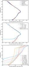 |
Fig. 4 Upper panel: influence of the hadronic interaction model on the computation of the Venusian ion-pair production rates. A comparison between the QGSP_BIC, QGSP_ BIC_HP, FTFP_ BERT and FTFP_BERT_HP models for primary protons between 1 MeV nuc−1 and 1 TeV nuc−1 is shown. In comparison, the proton-induced ionization rates by Nordheim et al. (2015) are displayed (dashed line). Middle panel: influence of the energy range on the GCR-induced ion-pair production based on the FTFP_ BERT_HP model for primary protons between 1 MeV–100 GeV, 1 MeV–1 TeV and 1 MeV–10 TeV. The results by Plainaki et al. (2016) are given in light blue. Lower panel: influence of primary protons of selected energy bins on the ion pair production rates at altitudes below 60 km (for further information see Sect. 4.1.3). |
4.2 Solar cosmic ray-induced ionization
The shape of the energy spectra of strong SEP events strongly differs from the spectra of GCRs. Although being orders of magnitudes higher at low particle energies their spectra most often are very steep and do not exceed a few GeV nuc−1. As previously discussed, strong SEP events may cause extensive particle showers within planetary atmospheres. However, because of particle acceleration and transport mechanisms, the energy spectrum of such events is temporally and spatially variable. Although remarkable efforts revealing the temporal evolution of SEP events can be found in literature (see, e.g., Belov et al. 2005; Bombardieri et al. 2007; Plainaki et al. 2007; Matthiä et al. 2009; Miroshnichenko 2018, and references therein) to model the atmospheric effects induced by solar energetic particles often a mean energy spectrum is used.
In order to study the mean influence of strong SEP events on the ion-pair production in a first step, the contribution of protons and heavier ions (Z = 2–28) during a series of intense events measured during the Neutron Monitor era (GLE43–GLE45, in October 1989) are investigated. Therefore, the spectra have been extracted from the CREME2009 model (Tylka et al. 1997). Following the investigations by Nordheim et al. (2015) and Dartnell et al. (2015), we have focussed on two specific scenarios: the peak scenario, corresponding to the 5 min average event peak flux measured with the GOES spacecraft on October 20, 1989 (secenario 1), and the average scenario corresponding to the particle fluxes averaged over 180 h starting at 1300 UTC on October 19, 1989 (scenario 2).
The results of scenario 1 and scenario 2 are shown in the upper and middle panels of Fig. 5, respectively. As can be seen in both panels, contrary to the case of the GCR-induced ionization, for this SEP event the results by Nordheim et al. (2015) and this study are in excellent agreement with each other. This further points out the treatment of high energy particles by different Geant4 versions and physics lists discussed in Sect. 4.1 as crucial factors. Furthermore, the middle panel shows the results by Plainaki et al. (2016, light blue line). Above an altitude of 60 km the results are in good agreement with Nordheim et al. (2015) and the results of this study. However, below an altitude of 60 km strong differences occur. These are most likely caused by numerical instabilities due to the applied energy binning.
A direct comparison to the GCR-induced production rates by Nordheim et al. (2015) and Plainaki et al. (2016) during solar minimum conditions is shown in the lower panel of Fig. 5. As can be seen, the SEP-induced ionization maxima are quite different from those of the GCR-induced background ionization. Thereby, the SEP-induced ionisation is up to four orders of magnitude higher than the ionization induced by GCRs. Also, it becomes obvious that GCRs and SEPs are the main driver of ion pair production in the Venusian atmosphere at altitudes below ~100 km. In the upper atmosphere, however, the day-time EUV/X-ray-induced ionization published by Peter et al. (2014, here for a low solar zenithal angle χ = 23.1°, displayed in green) dominates the atmospheric ionization above 100 km, with a peak maximum at around 140 km. Furthermore, the first two panels reveal that the influence of Z > 2 particles on the GLE-induced ionization is rather weak. Thus, investigating the influence of strong SEP events on the Venusian atmosphere can be restricted to modeling the influence of solar protons. Therefore, in what follows we present a detailed study on the influence of the 71 GLE events that occurred between 1942 and 2012 applying the Band-fit functions, that represent the mean event-integrated proton fluences, published by Raukunen et al. (2018). We would like to emphasize that we are not modeling the impact of these specific SEP events as they interacted with Venus. Rather, we are using these events (as recorded at Earth) as a case-study for the effect of SEP-induced ionization on the Venusian atmosphere. For each event, we have therefore assumed that the directional properties of the SEP particles have allowed their arrival and penetration into the Venusian atmosphere.
The impact of those GLE events is displayed in Fig. 6. Here the sum of the GCR-induced (solar maximum conditions, black dotted line) and the GLE-induced ion-pair production rate is plotted (colored lines). As can be seen, substantial differences of up to six orders of magnitude between the GLE-induced ion pair production rates occur, which are mainly caused by the different shapes of the GLE event spectra. As can be seen, GLE62 (November 4, 2001, magenta dashed line), is the event with the weakest influence on the Venusian atmosphere while GLE10 and GLE11 (November 12, 1960, and November 15, 1960, orange solid and dashed lines, respectively) induced the most severe production of ion pairs in the upper Venusian atmosphere above 120 km. Furthermore, the influence of GLE05 (February 23, 1956), the strongest GLE event ever measured in situ, is displayed as solid green line. Although its spectrum shows the highest intensities of all modern GLE events above 100 MeV, it does not result in the highest ion-pair production rate values. However, due to its very hard spectrum an ionization of much lower altitudes inside the Venusian atmosphere compared to all other GLE events is induced. For more details on the GLE-dependent peak altitudes and their corresponding ion-pair production rate values see Table 2.
Moreover, Fig. 6 also shows a unique feature of the Venusian atmosphere compared to other solar system planets: the Venusian ionization maximum is well within the cloud-producing altitudes. According to Yair (2012) the clouds of Venus are composed of small droplets or ice crystals of sulfuric acid, and reside in three distinct layers: the lower cloud region between 47 and 50 km, the middle region in between 50 and 57 km as well as the upper cloud region between 57 and 70 km (see, e.g., Horinouchi et al. 2017). Thus, as shown in this study, these altitudes are strongly affected by strong solar energetic particle events.
However, one has to keep in mind that strong SEP events can be accompanied by so-called Forbush decreases (FDs), sudden GCR-intensity decreases that are caused by interplanetary shocks or magnetized ejecta of coronal mass ejections (Cane 2000). In such cases, the ion pair production rate due to the background GCRs might therefore be reduced.
Moreover, GLE05 most likely was not the strongest GLE that ever occurred throughout the history of the Sun. On September 1, 1859 the so-calledCarrington-event followed a particularly intense solar white-light flare. Because of the atmospheric production of cosmogenic radionuclides like 14C, 10 Be and 36 Cl due to GCRs and SCRs and their storage in natural archives like ice sheets or organic material information on the solar activity of thousands of years is stored. Within records of the past ~10 000 yr an exceptionally strong production rate increase around AD775 has been found (see, e.g., Miyake et al. 2012; Mekhaldi et al. 2015). A remarkably strong GLE event may have induced this sudden increase. Model studies of the terrestrial cosmogenic radionuclide production showed that, for example, the event of AD775 was well over one order of magnitude stronger than GLE05 (see, e.g., Kovaltsov & Usoskin 2014; Herbst et al. 2015). In order to estimate an upper limit of the influence of such extreme events in the following, the two historical events are studied in more detail.
Unfortunately, we have no information about the differential intensity spectrum of these intense events. Thus, their spectral shape has to be modeled based on more recent SEP events. In this study, we use the spectral shapes published by Dartnell et al. (2015). These spectra were based on the Weibull distribution and parameters derived by Kim et al. (2009, for GLE05) and Xapsos et al. (2000, for the August 1972 and October 1989 events) the energy spectra have been computed. In addition, Dartnell et al. (2015) scaled the spectra for these events to match the estimated E > 30 MeV integral fluence of the Carrington Event (see, e.g., Cliver & Dietrich 2013) and the estimated E > 200 MeV integral fluence of the AD775 event (Kovaltsov & Usoskin 2014). The spectra are shown in the upper panel of Fig. 7. Here the spectra based on the shape of GLE05 are displayed in light blue, those based on the shape of the GLE of August 1972 in red, and the spectra utilizing the shape of the October 1989 event spectrum in blue.
However, to account for an averaged differential spectrum the duration of such an event has to be taken into account. Following the approach by Dartnell et al. (2015) we accounted for an event duration of 20 h, in which most of the event fluence was injected toward the Earth. We assumed the same SEP duration time for the AD775 event. The corresponding event-induced ion-pair production rate values are displayed in the lower panel. In addition, the corresponding values can be found in Table 3. Furthermore, here the ratio between the SEP- and GCR-induced ionization rates at the Venusian Pfotzer maximum (h = 64 km) are given. As can be seen, depending on the assumed spectral shape an the duration time both the Carrington event and the AD775 event could have been able to induce more than four orders of magnitude higher ionization rates at the GCR-induced Pfotzer maximum (64 km), and thus well within the cloud-covering regions. Thus, particularly strong solar events may have a strong influence on chemical and electrical processes within the Venusian atmosphere. However, because neither the actual spectral shape nor the temporal evolution of such historical events are known, the results presented here can only be seen as case studies that provide some upper- and lower-limits on the effect of such extreme SEP events.
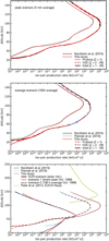 |
Fig. 5 Upper panel: altitude-dependent ion pair production rates for the 5 min average event peak flux measured with the GOES spacecraft on October 20, 1989 (scenario 1). A comparison to the results by Nordheim et al. (2015, black curve) is given. Middle panel: altitude-dependent ion pair production rates induced by the particle fluxes averaged over 180 h starting at 1300 UTC on October 19, 1989 (scenario 2). Here in addition to the results by Nordheim et al. (2015, in black) the results by Plainaki et al. (2016) are displayd as blue line. Lower panel: comparison of the GCR- and strong SEP event-induced Venusian ionization. In addition the upper altitude-ionization due to EUV and X-rays on the Venusian day-side is shown (green line; Peter et al. 2014). |
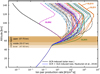 |
Fig. 6 Influence of modern ordinary strong SEP spectra on the Venusian ion-pair production rate values. Shown is the sum of the GCR- induced background ionization (taking into account protons up to 10 TeV) during solar maximum conditions and the SEP-induced production rates (colored lines). Of particular interest in this study are the four labeled events: GLE05 (green line), GLE10 (orange solid line), GLE11 (orange dashed line), and GLE62 (purple line). |
Estimates of the GLE-induced ion-pair production rate maxima (Q) and their corresponding altitudes of GLE05, GLE10, GLE11, and GLE62.
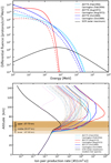 |
Fig. 7 Upper panel: differential fluence spectra of both historical extreme SEP events, the Carrington event (dashed lines) as well as the AD775 event (solid lines) based on the shape of three different modern SEP events: February 1956 (in light blue), August 1972 (in red), and October 1989 (in blue). In order to account for a differential flux spectrum the results have been scaled to an event duration of 20 h (see Dartnell et al. 2015, for further information). Lower panel: event-induced ion-pair production rates depending on the above-mentioned spectra. For comparison the production rate values of the 71 modern SEP events (see Fig. 6) are displayed as shaded curves. |
5 Summary and conclusions
With the newly developed simulation code AtRIS, based on full 3D Monte Carlo modeling, in this study, we provide updated cosmic ray induced Venusian ionization profiles. The newest numerical physics models (Geant4 10.5, FTFP_BERT_HP) have been used and GCR intensities of Z = 1–28 particles in the energy range of 1 MeV nuc−1 to 1 TeV nuc−1 have been modeled. In addition, we have investigated the effect of SEP-induced atmospheric ionization by considering 71 space-age and two historical SEP events as case studies.
The results of our study show that around the Pfotzer maximum our ion-pair production rates are in reasonably good agreement to the full 3D modeling efforts by Nordheim et al. (2015) and Plainaki et al. (2016) as well as the analytical studies by Dubach et al. (1974) and Borucki et al. (1982). However, substantial differences occur in altitudes above 120 km and below 40 km. Therefore, the influence of the applied Geant4 version, the different hadronic interaction models, as well as the upper energy limit, has been studied. We show that the differences in the upper and lower atmosphere most likely are caused by the updates of both the Fritiof and Quark-Gluon-String model implemented in the Geant4 10.5 release. Furthermore, we have demonstrated that primary GCR protons should be modeled up to at least 10 TeV energies since primary protons between 1 and 10 TeV cause more than one order of magnitude higher ion-pair production rates at altitudes below 20 km.
Furthermore, we show that model efforts studying the influence of strong SEP events on the Venusian atmosphere can be restricted tomodeling the influence of solar protons. Therefore, we have evaluated the influence of 71 strong solar energetic proton events that have been measured at the Earth’s surface between 1942 and 2012 (see Raukunen et al. 2018). As we show, there have been events (e.g., GLE10 and GLE11) which would have induced high-altitude ion-pair production rates in the order of eleven orders of magnitude higher than induced by GCRs during solar maximum conditions. While most of these events would not have significantly affected ionization rates below the Venusian GCR-induced production (Pfotzer) maximum around 64 km, the SEP event of of February 23, 1956, the strongest GLE ever measured, would have lead to a mean ionization rate increase at these altitudes of up to three orders of magnitude. Moreover, from historical records, such as those of the cosmogenic radionuclides (10 Be, 14 C and, 36 Cl), we know that the Sun most likely produced much stronger SEP events than what has been observed over the past seven decades (see, e.g., Miyake et al. 2012; Mekhaldi et al. 2015; O’Hare et al. 2019). In agreement with Dartnell et al. (2015) we have shown that such intense sporadic events have a strong influence on altitudes well below the GCR-induced ionization maximum and can lead to ionization rates that are in the order of six orders of magnitudes higher than the GCR-induced ionization background.
For most of the historical GLE events considered in this paper, neither the actual spectral shape nor the temporal evolution of the particle flux are known. Thus, the results presented here should be seen as case studies that provide possible upper- and lower- limits on the effect of such extreme SEP events, assuming a priori that the directional properties of the particles have allowed their arrival and penetration to the Venusian atmosphere. However, several SEP/GLE events and their properties at 1 AU, have been long studied through sophisticated back-tracing techniques based on data from the worldwide neutron monitor network (see, e.g., Belov et al. 2005; Bombardieri et al. 2007; Plainaki et al. 2007, 2014, and references therein). These studies have revealed the characteristics of the temporal evolution of the SEP spectrum at a distance of 1 AU, providing information on the spatial distribution of the flux at the top of the terrestrial atmosphere. In case of Venus, Plainaki et al. (2016) were the first to consider a SEP spectrum based on data-modeling results for a specific GLE event observed at Earth to estimate the ion pair production rate profile. Although the latter study was based on a comparative planetology approach, it was only focused on two specific SEP events and further studies are mandatory. The results presented in the study, therefore, integrate the previous efforts by Nordheim et al. (2015) and Plainaki et al. (2016) setting important constraints on the expected planetary space weather impact on Venus.
From the terrestrial atmosphere, we know that GCRs create cluster-ions that play a significant role in meteorological processes (Mironova et al. 2015). According to Yair (2012) the clouds of Venus are composed of small droplets or ice crystals of sulfuric acid, and reside in three distinct layers: the lower cloud region between 47 and 50 km, the middle region in between 50 and 57 km as well as the upper cloud region between 57 and 70 km (see, e.g., Horinouchi et al. 2017). Due to its proximity to the Sun, the Venusian cloud-producing altitudes are strongly affected by space weather. Thus, it is believed that the majority of the cloud particles are charged by GCRs (Michael et al. 2009) and that the ionization caused by these particles could influence the cloud formation rates in the Venusian atmosphere (Aplin 2006, 2013). As shown, the ionization maximum is well within the main cloud deck. Thus, the Venusian clouds are charged continuously and separated by local electric fields (see, e.g., Aplin et al. 2017). According to Borucki et al. (1982) the primary ions formed in the Venusian atmosphere are CO , CO+ as well as O+ which are converted into ion clusters that further influence the Venusian chemistry. Furthermore, as on Earth, a possible consequenceof the atmospheric ionization could be the presence of lightning generated by the separation of electric charge residing on water-ice particles within the cloud layers. A recent detailed discussion of the evidence of optical lightning can be found in Titov et al. (2018).
However, the magnetometer aboard the Venus Express mission has repeatedly measured whistler waves, electromagnetic waves caused by lightning (see, e.g., Russell et al. 2007, 2011). Moreover, Gray et al. (2014) studied the oxygen green line nightglow emissions with the high resolution Astrophysical Research Consortium Echelle Spectrograph on the Apache Point Observatory3.5 m telescope from December 2010 to July 2012. They found the emissions to be a result of an enhanced solar wind electron precipitation caused by the passage of interplanetary coronal mass ejections as well as SEP events.
Although our study shows that most of the modern strong solar energetic particle events would have had only a minor influence within the altitudes of the cloud layers, strong SEP events such as the Ground Level Enhancement of February 23, 1956 (GLE05) would lead to an ionization rate enhancement of three orders of magnitude. Furthermore, both the Carrington event and the AD775 event, two estimated historical extreme SEP events (based on an averaged event duration of 20 h) would have induced an ionization rate within the Venusian cloud deck that is six orders of magnitude higher than the background GCR value. However, we note that the duration of such an event could in reality have been rather different than we have assumed here. Nevertheless, it is clear that particularly strong solar events may have a significant influence on chemical and electrical processes inside the Venusian atmosphere.
Estimates of the SEP-induced ion-pair production rate maxima (in units of ions (cm3 s)−1) and their corresponding altitudes (in units of km) of both historical extreme SEP events, the Carrington and AD775 events based on the spectral shapes of the February, 1956, August 1972, and October 1989 events.
Acknowledgements
K.H. acknowledges the International Space Science Institute and the supported International Team 441: High EneRgy sOlar partICle Events Analysis (HEROIC). S.B. thanks the German Research Foundation (DFG) for financial support via the project The Influence of Cosmic Rays on Exoplanetary Atmospheric Biosignatures (Project number 282759267). Furthermore, K.H. and S.B. thank Bernd Heber for fruitful discussions. Work by T.A.N. was carried out at the Jet Propulsion Laboratory, California Institute of Technology, under a contract with the National Aeronautics and Space Administration.
References
- Allison, J., Amako, K., Apostolakis, J., et al. 2016, Nucl. Instrum. Methods Phys. Res. A, 835, 186 [NASA ADS] [CrossRef] [Google Scholar]
- Aplin, K. 2006, Surv. Geophys., 27, 63 [NASA ADS] [CrossRef] [Google Scholar]
- Aplin, K. L. 2013, Venus (Dordrecht, The Netherlands: Springer), 13 [Google Scholar]
- Aplin, K., Airey, M., & Warriner-Bacon, E. 2017, ArXiv e-prints [arXiv:1705.05597] [Google Scholar]
- Banjac, S., Herbst, K., & Heber, B. 2019, J Geophys. Res., 124, 50 [Google Scholar]
- Bazilevskaya, G. A., Usoskin, I. G., Flückiger, E. O., et al. 2008, Space Sci. Rev., 137, 149 [Google Scholar]
- Belov, A., Eroshenko, E., Mavromichalaki, H., Plainaki, C., & Yanke, V. 2005, Ann. Geophys., 23, 2281 [NASA ADS] [CrossRef] [Google Scholar]
- Bombardieri, D. J., Michael, K. J., Duldig, M. L., & Humble, J. E. 2007, ApJ, 665, 813 [Google Scholar]
- Borucki, W., Levin, Z., Whitten, R., & Keesee, R. 1982, Icarus, 321, 302 [NASA ADS] [CrossRef] [Google Scholar]
- Büsching, I., Kopp, A., Pohl, M., et al. 2005, ApJ, 619, 314 [NASA ADS] [CrossRef] [Google Scholar]
- Cane, H. V. 2000, Space Sci. Rev., 93, 55 [NASA ADS] [CrossRef] [Google Scholar]
- Cliver, E. W., & Dietrich, W. F. 2013, J. Space Weather Space Clim., 3, A31 [CrossRef] [EDP Sciences] [Google Scholar]
- Dartnell, L., Nordheim, T. A., Patel, M. R., et al. 2015, Icarus, 257, 396 [NASA ADS] [CrossRef] [Google Scholar]
- Desorgher, L., Flückiger, E. O., & Gurtner, M. 2006, in 36th COSPAR Scientific Assembly, 36, 2361 [NASA ADS] [Google Scholar]
- Dubach, J., Whitten, R., & Sims, J. 1974, Planet. Space Sci., 22, 525 [NASA ADS] [CrossRef] [Google Scholar]
- Forget, F., Millour, E., Lebonnois, S., et al. 2006, Second workshop on Mars atmosphere modelling and observations, 27 Feb–3 Mar 2006, Granada, Spain [Google Scholar]
- Fox, J. L., Galand, M. I., & Johnson, R. E. 2008, Space Sci. Rev., 139, 3 [NASA ADS] [CrossRef] [Google Scholar]
- Geant4 Collaboration 2018, Geant4 guide for physics lists, https://geant4.web.cern.ch/support/user_documentation [Google Scholar]
- Gieseler, J., & Heber, B. 2016, A&A, 589, A32 [NASA ADS] [CrossRef] [EDP Sciences] [Google Scholar]
- Gray, C. L., Chanover, N. J., Slanger, T. G., & Molaverdikhani, K. 2014, Icarus, 233, 342 [NASA ADS] [CrossRef] [Google Scholar]
- Guo, J., Banjac, S., Röstel, L., et al. 2019, J. Space Weather Space Clim., 9, A2 [CrossRef] [EDP Sciences] [Google Scholar]
- Heber, B., Droege, W., Ferrando, P., et al. 1996, A&A, 316, 538 [NASA ADS] [Google Scholar]
- Herbst, K., Kopp, A., & Heber, B. 2013, Ann. Geophys., 31, 1637 [Google Scholar]
- Herbst, K., Heber, B., Beer, J., & Tylka, A. J. 2015, The 34th International Cosmic Ray Conference, The Hague, PoS, 537 [Google Scholar]
- Hillas, A. M. 2005, Phys. G Nucl. Part. Phys., 31, R95 [Google Scholar]
- Horinouchi, T., Murakami, S.-y., Satoh, T., et al. 2017, Nat. Geosci., 10, 646 [NASA ADS] [CrossRef] [Google Scholar]
- ICRU 1993, ICRU Publications, Washington, DC, Report No. 31 [Google Scholar]
- Keating, G., Bertaux, J., Bougher, S., et al. 1985, Adv. Space Res., 5, 117 [NASA ADS] [CrossRef] [Google Scholar]
- Kim, M. Y., Hayat, M. J., Feiveson, A. H., & Cucinotta, F. A. 2009, Health Phys., 97, 68 [CrossRef] [Google Scholar]
- Kliore, A. J., Keating, G. M., & Moroz, V. I. 1992, Planet. Space Sci., 40, 573 [NASA ADS] [CrossRef] [Google Scholar]
- Kovaltsov, G. A., & Usoskin, I. G. 2014, Sol. Phys., 289, 211 [NASA ADS] [CrossRef] [Google Scholar]
- Luhmann, J., Ledvina, S., & Russell, C. 2004, Adv. Space Res., 33, 1905 [NASA ADS] [CrossRef] [Google Scholar]
- Matthiä, D., Heber, B., Reitz, G., et al. 2009, J. Geophys. Res. Space Phys., 114, A08104 [NASA ADS] [CrossRef] [Google Scholar]
- Mekhaldi, F., Muscheler, R., Adolphi, F., et al. 2015, Nat. Commun., 6, 8611 [NASA ADS] [CrossRef] [Google Scholar]
- Michael, M., Tripathi, S. N., Borucki, W. J., & Whitten, R. C. 2009, J. Geophys. Res. Planets, 114, E4 [CrossRef] [Google Scholar]
- Mironova, I. A., Aplin, K. L., Arnold, F., et al. 2015, Space Sci. Rev., 194, 1 [NASA ADS] [CrossRef] [Google Scholar]
- Miroshnichenko, L. I. 2018, J. Space Weather Space Clim., 8, A52 [NASA ADS] [CrossRef] [EDP Sciences] [Google Scholar]
- Miyake, F., Nagaya, K., Masuda, K., & Nakamura, T. 2012, Nature, 486, 240 [NASA ADS] [CrossRef] [Google Scholar]
- Morales-Olivares, O., & Caballero-Lopez, R. 2010, Adv. Space Res., 46, 1313 [NASA ADS] [CrossRef] [Google Scholar]
- Nilsson-Almqvist, B., & Stenlund, E. 1987, Comput. Phys. Commun., 43, 387 [NASA ADS] [CrossRef] [Google Scholar]
- Nordheim, T. A., Dartnell, L., Desorgher, L., Coates, A., & Jones, G. 2015, Icarus, 245, 80 [NASA ADS] [CrossRef] [Google Scholar]
- O’Hare, P., Mekhaldi, F., Adolphi, F., et al. 2019, Proc. Natl. Acad. Sci., 116, 5961 [NASA ADS] [CrossRef] [Google Scholar]
- Paschalis, P., Mavromichalaki, H., Dorman, L., Plainaki, C., & Tsirigkas, D. 2014, New Astron., 33, 26 [NASA ADS] [CrossRef] [Google Scholar]
- Peter, K., Pätzold, M., Molina-Cuberos, G., et al. 2014, Icarus, 233, 66 [NASA ADS] [CrossRef] [Google Scholar]
- Pfotzer, G. 1936, Z. Phys., 102, 41 [NASA ADS] [CrossRef] [Google Scholar]
- Phillips, J. L.,& Russell, C. T. 2012, J. Geophys. Res., 92, 2253 [Google Scholar]
- Picone, J., Hedin, A., Drob, D. P., & Aikin, A. 2002, J. Geophys. Res. Space Phys., 107, A12 [Google Scholar]
- Plainaki, C., Belov, A., Eroshenko, E., Mavromichalaki, H., & Yanke, V. 2007, J. Geophys. Res. Space Phys., 112 [Google Scholar]
- Plainaki, C., Mavromichalaki, H., Laurenza, M., et al. 2014, ApJ, 785, 160 [Google Scholar]
- Plainaki, C., Paschalis, P., Grassi, D., Mavromichalaki, H., & Andriopoulou, M. 2016, Ann. Geophys., 34, 595 [NASA ADS] [CrossRef] [Google Scholar]
- Raukunen, O., Vainio, R., Taylka. A. J., et al. 2018, J. Space Weather Space Clim., 8, A04 [CrossRef] [EDP Sciences] [Google Scholar]
- Reames, D. V. 1999, Space Sci. Rev., 90, 413 [Google Scholar]
- Russell, C. T., Elphic, R. C., & Slavin, J. A. 1979, Science, 203, 745 [NASA ADS] [CrossRef] [Google Scholar]
- Russell, C., Luhmann, J., & Strangeway, R. 2006, Planet. Space Sci., 54, 1482 [NASA ADS] [CrossRef] [Google Scholar]
- Russell, C. T., Zhang, T. L., Delva, M., et al. 2007, Nature, 450, 661 EP [NASA ADS] [CrossRef] [PubMed] [Google Scholar]
- Russell, C., Strangeway, R., Daniels, J., Zhang, T., & Wei, H. 2011, Planet. Space Sci., 59, 965 [NASA ADS] [CrossRef] [Google Scholar]
- Russell, C. T., Elphic, R. C., & Slavin, J. A. 2012, J. Geophys. Res., 85, 8319 [NASA ADS] [CrossRef] [Google Scholar]
- Schmelz, J. T., Reames, D. V., von Steiger, R., & Basu, S. 2012, ApJ, 755, 33 [NASA ADS] [CrossRef] [Google Scholar]
- Seiff, A., Schofield, J., Kliore, A., et al. 1985, Adv. Space Res., 5, 3 [NASA ADS] [CrossRef] [Google Scholar]
- Simon Wedlund, C., Gronoff, G., Lilensten, J., Ménager, H., & Barthélemy, M. 2011, Ann. Geophys., 29, 187 [NASA ADS] [CrossRef] [Google Scholar]
- Sinnhuber, M., Berger, U., Funke, B., et al. 2018, Atmos. Chem. Phys., 18, 1115 [Google Scholar]
- Svedhem, H., Titov, D. V., Taylor, F. W., & Witasse, O. 2007, Nature, 450, 629 EP [NASA ADS] [CrossRef] [Google Scholar]
- Taylor, F. W., Svedhem, H., & Head, J. W. 2018, Space Sci. Rev., 214, 35 [NASA ADS] [CrossRef] [Google Scholar]
- Titov, D. V., Ignatiev, N. I., McGouldrick, K., Wilquet, V., & Wilson, C. F. 2018, Space Sci. Rev., 214, 126 [NASA ADS] [CrossRef] [Google Scholar]
- Tylka, A. J., Adams, J. H., Boberg, P. R., et al. 1997, IEEE Trans. Nucl. Sci., 44, 2150 [Google Scholar]
- Upadhyay, H., & Singh, R. 1995, Adv. Space Res., 15, 99 [NASA ADS] [CrossRef] [Google Scholar]
- Upadhyay, H., Singh, R., & Singh, R. 1994, Earth Moon Planets, 65, 89 [NASA ADS] [CrossRef] [Google Scholar]
- Vech, D., Szego, K., Opitz, A., et al. 2015, J. Geophys. Res. Space Phys., 120, 4613 [NASA ADS] [CrossRef] [Google Scholar]
- Vinogradov, A., Surkov, Y., & Kirnozov, F. 1973, Icarus, 20, 253 [NASA ADS] [CrossRef] [Google Scholar]
- Xapsos, M. A., Barth, J. L., Stassinopoulos, E. G., et al. 2000, IEEE Trans. Nucl. Sci., 47, 2218 [NASA ADS] [CrossRef] [Google Scholar]
- Yair, Y. 2012, Adv. Space Res., 50, 293 [NASA ADS] [CrossRef] [Google Scholar]
- Zhang, T. L., Delva, M., Baumjohann, W., et al. 2008, J. Geophys. Res. Planets, 113 [Google Scholar]
Available at https://creme.isde.vanderbilt.edu/
For more detailed version-dependent information the reader is referred to https://github.com/Geant4/geant4/releases
All Tables
Estimates of the altitude hmax (km) and the ion pair production rate Q of the Venusian Pfotzer maximum during solar minimum (solar maximum) conditions modeled by Dubach et al. (1974, DU74), Borucki et al. (1982, BO82), Upadhyay & Singh (1995, US95), Nordheim et al. (2015, NO15), Plainaki et al. (2016, PL16) and this work (HE19).
Estimates of the GLE-induced ion-pair production rate maxima (Q) and their corresponding altitudes of GLE05, GLE10, GLE11, and GLE62.
Estimates of the SEP-induced ion-pair production rate maxima (in units of ions (cm3 s)−1) and their corresponding altitudes (in units of km) of both historical extreme SEP events, the Carrington and AD775 events based on the spectral shapes of the February, 1956, August 1972, and October 1989 events.
All Figures
|
Fig. 1 Sketch of the altitude-dependent evolution of a secondary particle cascade induced by a high-energy primary cosmic ray particle (Z = 1–28). The cascade develops three branches: the electromagnetic branch mainly consisting of electrons, positrons and photons (also known as “soft component”), the muonic branch (the “hard component”), as well as the hadronic branch, mainly consisting of neutrons and protons (see, e.g., Bazilevskaya et al. 2008). |
| In the text | |
|
Fig. 2 Atmospheric profile based on the VIRA model (see Keating et al. 1985; Seiff et al. 1985) used in this study. Left panel: altitude-dependent temperature (black line) and density profile (red line). Right panel: corresponding atmospheric depth (black line) and pressure profiles (red line). |
| In the text | |
|
Fig. 3 Upper left panel: altitude-dependent total ion pair production rates during solar minimum conditions at Venus (thisstudy, red solid line) and at Earth (blue line, see Banjac et al. 2019) as a reference. The following panels only address the Venusian ionization. Upper right panel: influence of the applied ionization potential w. Shown here are the model results for the w-values by Borucki et al. (1982, w = 33.5 eV, red solid line) and Simon Wedlund et al. (2011, w = 28.7 ± 4.3 eV, red dashed line and corresponding error band). Lower left panel: contribution of Z = 1 (protons, dashed lines) and Z = 2–28 (dotted lines) particles to the total atmospheric ionization (solid line) during solar minimum conditions. The results by Nordheim et al. (2015, black curves) are compared to the results of this study (red curves). Lower right panel: comparison of the altitude-dependent ionization rates by Plainaki et al. (2016, light blue curves) and the results of our study during solar minimum (solid lines) and solar maximum (dashed lines) conditions. In addition the results by Dubach et al. (1974; blue), Borucki et al. (1982, orange), and Upadhyay & Singh (1995; purple) are displayed. |
| In the text | |
|
Fig. 4 Upper panel: influence of the hadronic interaction model on the computation of the Venusian ion-pair production rates. A comparison between the QGSP_BIC, QGSP_ BIC_HP, FTFP_ BERT and FTFP_BERT_HP models for primary protons between 1 MeV nuc−1 and 1 TeV nuc−1 is shown. In comparison, the proton-induced ionization rates by Nordheim et al. (2015) are displayed (dashed line). Middle panel: influence of the energy range on the GCR-induced ion-pair production based on the FTFP_ BERT_HP model for primary protons between 1 MeV–100 GeV, 1 MeV–1 TeV and 1 MeV–10 TeV. The results by Plainaki et al. (2016) are given in light blue. Lower panel: influence of primary protons of selected energy bins on the ion pair production rates at altitudes below 60 km (for further information see Sect. 4.1.3). |
| In the text | |
|
Fig. 5 Upper panel: altitude-dependent ion pair production rates for the 5 min average event peak flux measured with the GOES spacecraft on October 20, 1989 (scenario 1). A comparison to the results by Nordheim et al. (2015, black curve) is given. Middle panel: altitude-dependent ion pair production rates induced by the particle fluxes averaged over 180 h starting at 1300 UTC on October 19, 1989 (scenario 2). Here in addition to the results by Nordheim et al. (2015, in black) the results by Plainaki et al. (2016) are displayd as blue line. Lower panel: comparison of the GCR- and strong SEP event-induced Venusian ionization. In addition the upper altitude-ionization due to EUV and X-rays on the Venusian day-side is shown (green line; Peter et al. 2014). |
| In the text | |
|
Fig. 6 Influence of modern ordinary strong SEP spectra on the Venusian ion-pair production rate values. Shown is the sum of the GCR- induced background ionization (taking into account protons up to 10 TeV) during solar maximum conditions and the SEP-induced production rates (colored lines). Of particular interest in this study are the four labeled events: GLE05 (green line), GLE10 (orange solid line), GLE11 (orange dashed line), and GLE62 (purple line). |
| In the text | |
|
Fig. 7 Upper panel: differential fluence spectra of both historical extreme SEP events, the Carrington event (dashed lines) as well as the AD775 event (solid lines) based on the shape of three different modern SEP events: February 1956 (in light blue), August 1972 (in red), and October 1989 (in blue). In order to account for a differential flux spectrum the results have been scaled to an event duration of 20 h (see Dartnell et al. 2015, for further information). Lower panel: event-induced ion-pair production rates depending on the above-mentioned spectra. For comparison the production rate values of the 71 modern SEP events (see Fig. 6) are displayed as shaded curves. |
| In the text | |
Current usage metrics show cumulative count of Article Views (full-text article views including HTML views, PDF and ePub downloads, according to the available data) and Abstracts Views on Vision4Press platform.
Data correspond to usage on the plateform after 2015. The current usage metrics is available 48-96 hours after online publication and is updated daily on week days.
Initial download of the metrics may take a while.