| Issue |
A&A
Volume 624, April 2019
|
|
|---|---|---|
| Article Number | A63 | |
| Number of page(s) | 21 | |
| Section | Galactic structure, stellar clusters and populations | |
| DOI | https://doi.org/10.1051/0004-6361/201935061 | |
| Published online | 11 April 2019 | |
Near-infrared spectroscopy of the massive stellar population of W51: evidence for multi-seeded star formation⋆,⋆⋆,⋆⋆⋆
1
Department of Astronomy, Stockholm University, AlbaNova University Centre, 106 91 Stockholm, Sweden
e-mail: This email address is being protected from spambots. You need JavaScript enabled to view it.
2
Max-Planck-Institut für Astronomie, Königstuhl 17, 69117 Heidelberg, Germany
3
Astronomisches Rechen-Institut, Zentrum für Astronomie der Universität Heidelberg, Mönchhofstr. 12–14, 69120 Heidelberg, Germany
4
Argelander Institut für Astronomie, Auf dem Hügel 71, 53121 Bonn, Germany
Received:
15
January
2019
Accepted:
14
February
2019
Abstract
Context. The interplay between the formation of stars, stellar feedback and cloud properties strongly influences the star formation history of giant molecular clouds. The formation of massive stars leads to a variety of stellar clusters, ranging from low stellar density OB associations to dense, gravitationally bound starburst clusters.
Aims. We aimed at identifying the massive stellar content and reconstructing the star formation history of the W51 giant molecular cloud.
Methods. We performed near-infrared imaging and K-band spectroscopy of the massive stars in W51. We analysed the stellar populations using colour-magnitude and colour-colour diagrams and compared the properties of the spectroscopically identified stars with stellar evolution models.
Results. We derive the ages of the different sub-clusters in W51 and, based on our spectroscopy derive an age for W51 of 3 Myr or less. The age of the P Cygni star LS1 and the presence of two still forming proto-clusters suggests that the star formation history of W51 is more complex than a single burst.
Conclusions. We did not find evidence for triggered star formation and we concluded that the star formation in W51 is multi seeded. We finally concluded that W51 is an OB association where different sub-clusters form over a time span of at least 3–5 Myr.
Key words: stars: formation / stars: early-type / techniques: spectroscopic / Hertzsprung-Russell and C-M diagrams / open clusters and associations: individual: W51 / infrared: stars
The photometry tables and the reduced spectra (FITS files) are only available at the CDS via anonymous ftp to cdsarc.u-strasbg.fr(130.79.128.5) or via http://cdsarc.u-strasbg.fr/viz-bin/qcat?J/A+A/624/A63
Based on data acquired using the Large Binocular Telescope (LBT). The LBT is an international collaboration among institutions in Germany, Italy and the United States. LBT Corporation partners are: LBT Beteiligungsgesellschaft, Germany, representing the Max Planck Society, the Astrophysical Institute Potsdam, and Heidelberg University; Instituto Nazionale di Astrofisica, Italy; The University of Arizona on behalf of the Arizona university system; The Ohio State University, and The Research Corporation, on behalf of The University of Notre Dame, University of Minnesota and University of Virginia.
Based on observations made with ESO Telescopes at the La Silla Paranal Observatory under programme ID 079.C-0248(A).
International Max Planck Research School for Astronomy and Cosmic Physics at the University of Heidelberg (IMPRS-HD).
© ESO 2019
1. Introduction
Stars form deeply embedded in giant molecular clouds (GMCs), and especially the formation process of massive stars is still a subject of debate (e.g. Zinnecker & Yorke 2007; Tan et al. 2014). What has become clear is that stars do not form isolated but in stellar clusters and associations (e.g. Lada & Lada 2003; Krumholz 2014). This means that the forming massive stars interact with each other by means of stellar feedback, where the first generation of star formation affects future generations of star formation in the same cloud (e.g. Krumholz et al. 2014).
The star formation process is hierarchical, driven by the self similar distribution of the dense gas in the molecular clouds (e.g. Elmegreen 2008, 2009). This results in different observed properties of star forming regions. Young star clusters with high stellar densities are in general found to be gravitationally bound (e.g. Stolte et al. 2004, 2006, 2008; Ascenso et al. 2007; Brandner et al. 2008; Rochau et al. 2010; Harfst et al. 2010; Gennaro et al. 2011; Hussmann et al. 2012). On the other side of the hierarchical spectrum extended, low-stellar density OB associations are found (e.g. Blaauw 1991; de Zeeuw et al. 1999; Comerón et al. 2002; Preibisch et al. 2011). The star formation histories of these star forming regions suggest that the star clusters such as Westerlund 1 and NGC 3606 consist of a single age population (e.g. Clark et al. 2005; Negueruela et al. 2010; Kudryavtseva et al. 2012), while less compact clusters such as the ONC (Palla & Stahler 1999; Da Rio et al. 2010), W3 Main (Feigelson & Townsley 2008; Bik et al. 2012) show evidence of an age spread of several Myr. In larger OB associations, such as the Orion OB association and Cyg OB2 much large age differences between OB subgroups are measured. In the case of Orion an age difference of at least 12 Myr (Brown et al. 1994; Bally 2008) is present, while analysis of the massive stars in Cyg OB2 shows that star formation has been going on for at least 10 Myr (Comerón & Pasquali 2012; Berlanas et al. 2018). Also older populations have been found associated with starburst clusters such as NGC 3603, where low-mass pre-main-sequence (PMS) stars up to ages of 10 Myr have been identified (Beccari et al. 2010) as well as two evolved supergiants with an age of 4 Myr (Melena et al. 2008). The observation that the age difference between the stars increases with the size of the observed structure can be explained by the hypothesis that star formation happens in a crossing time (Elmegreen 2000).
Kinematical studies based on proper motions confirm this fundamental difference between OB associations and starburst clusters. The starburst clusters consist of a single stellar population and their kinematics show typically a low velocity dispersion (Stolte et al. 2008; Rochau et al. 2010; Hussmann et al. 2012). OB associations on the other hand show more complicated kinematics. Wright et al. (2016) showed, based on multiple epoch imaging, that the Cyg OB2 association consists of multiple subgroups moving at different velocities and directions. The kinematics suggest that the stars are formed in situ as a result of multiple small scale star formation events. This result is inconsistent with OB associations being expanding clusters (e.g. Baumgardt & Kroupa 2007). With Gaia (Gaia Collaboration 2016), the in situ star formation scenario has been confirmed for other OB associations (Wright & Mamajek 2018; Ward & Kruijssen 2018; Kuhn et al. 2019).
The differences in morphology and star formation history will have a strong impact on how the feedback of the forming stars act on the molecular cloud (e.g. Rey-Raposo et al. 2017; Kim et al. 2018). Feedback influences future generations of stars by triggering new episodes of star formation or destroying the molecular cloud. Therefore a detailed understanding of the physical processes and stellar content in different GMC environments is important to understand how star formation progresses in different environments.
With the LOBSTAR project we are aiming at studying the stellar content of some of the most luminous HII regions in our Galaxy in order to trace back their formation history. We obtain high signal-to-noise ratio (S/N) K-band spectra of the massive stars and deep near-infrared imaging of these regions. In Bik et al. (2012, 2014) we presented evidence of an age spread of a few Myr in the stellar population of W3Main and showed that the high UV flux of the massive stars affects the circumstellar disks around the young stars. In W49, Wu et al. (2014) discovered one of the few known very massive stars (VMS) with a photometrically estimated mass between 100 and 180 M⊙. Wu et al. (2016) performed a spectral analysis of 14 O-type stars in W49 and concluded that the cluster has an age of ∼1.5 Myr.
This paper focusses on the last of the observed regions: W51. The W51 GMC complex is an elongated molecular cloud complex, located in the Sagittarius spiral arm at a distance of  kpc (Sato et al. 2010). W51 is one of the few GMC complexes in our galaxy with a mass above 106M⊙ (Carpenter & Sanders 1998) and spans a region on the sky of 45′ × 50′, corresponding to 70 × 80 pc. W51 consists of three parts; W51A is located in the north-east (high galactic longitude), W51B is located in the south-west (low galactic longitude) and W51C, a supernova remnant (Koo et al. 1995; Koo & Moon 1997; Brogan et al. 2013), is located towards the south-east of the complex. An observational review of the W51 complex can be found in Ginsburg (2017).
The region of most active star formation in W51 is the W51A cloud. This cloud has a much higher fraction of dense gas than W51B (Ginsburg et al. 2015) and hosts two of the only few known proto-clusters able to form a 104M⊙ or higher star cluster (Ginsburg et al. 2012). W51A was originally identified as a luminous radio source (Westerhout 1958). High resolution VLA observations have resolved W51A in many compact HII regions (Martin 1972; Scott 1978; Mehringer 1994; Ginsburg et al. 2016). Additionally several HII regions are found in W51B as well as radio emission towards the supernova remnant W51C (Koo & Moon 1997). W51 has been studied in molecular transitions such as CO (Carpenter & Sanders 1998; Kang et al. 2010; Fujita et al. 2017), H I (Koo & Moon 1997) and several other more complex molecules.
The stellar populations of the entire W51 GMC are analysed in detail in several near-infrared imaging studies. Most observations focus on the central regions of the W51A cloud where Neugebauer et al. (1969) and Wynn-Williams et al. (1974) detected several bright infrared sources, which were resolved in small clusters in higher spatial resolution imaging (Goldader & Wynn-Williams 1994). Okumura et al. (2000) studied the stellar content of the entire W51A cloud using near-infrared JHK′ and Brγ imaging. They identified several candidate OB stars and presented evidence for a top heavy initial mass function (IMF). Four subgroups have been found, ranging in age between 1 and 2.2 Myr. Nanda Kumar et al. (2004) observed 6 fields in the W51 GMC, including W51B, centred on the suspected location of embedded clusters based on 21 cm radio emission (Koo & Moon 1997), MSX and 2MASS data. Figuerêdo et al. (2008) obtained low resolution K-band spectra for five objects in the region of W51A, and could classify four of them as O-type stars. High resolution K-band spectra of two massive stars (associated with IRS2E and IRS2W, respectively) were obtained by Barbosa et al. (2008) in W51d, one of the compact HII regions in W51A. IRS2E was identified as a young stellar object (YSO), and IRS2W – which turns out to be the main ionizing source of W51d – was classified as an early O-type star (Barbosa et al. 2008).
Additional to the candidate OB stars, Okumura et al. (2000) identified two stars which are more luminous than the typical OB stars in W51. Both sources (LS1 and LS2) show an emission line spectrum. Based on the observed emission lines of Brγ, He I and Mg II in the K-band spectrum of LS1, the authors concluded that LS1 is a very massive P Cygni-type supergiant. Detailed modelling of a higher spectral resolution K-band spectrum by Clark et al. (2009) confirmed this conclusion, although the object is significantly less massive (∼40 M⊙) than the mass reported by Okumura et al. (2000). Spitzer imaging shows that the source is surrounded by a wind blown bubble. Clark et al. (2009) showed that the spectral identification as P Cygni supergiant places the objects at the distance of W51. Under the assumption that LS1 is part of the W51 cloud, Clark et al. (2009) showed that the age of the LS1 suggests that star formation has been active in W51 for at least 3 Myr. LS2 shows Brγ emission and could be either a B[e] supergiant or a young star surrounded by a circimstellar disk (Okumura et al. 2000).
The more embedded stellar content is traced with Spitzer, Herschel and SOFIA observations. Spitzer observations reveal hundreds of YSOs associated with the W51 cloud (Saral et al. 2017) distributed in several sub-clusters. They identified 17 massive YSO candidates and found that their locations correlate with the H II regions detected in the radio. Eden et al. (2018) presented Herschel and JCMT observations revealing a large sample of mm point sources in both W51 and W49A. They showed that the luminosity distribution of embedded sources in W51 and W49A are different. W51 has a luminosity function which is similar to the galactic average, while W49A shows an excess in bright sources, suggesting that the physical conditions in the central region of the W49A cloud could be different than in W51 and represents a more extreme mode of star formation. Using SOFIA imaging at 20 and 37 μm Lim & De Buizer (2019) studied the central areas of W51A at resolution of 2.2″ (20 μm) to 3.0″ (37 micron). They detected the dusty cocoons around the HII regions observed in the radio, showing that many HII regions are still deeply embedded. By combining the SOFIA imaging with Spitzer and Herschel, they identified 41 candidate massive YSOs. This demonstrates the very young nature of W51A.
The HII regions hosting the most important stellar clusters in W51A are called G49.5–0.4 and G49.4–0.3 of which the latter is hosting the two proto-cluster regions W51IRS2 and W51Main (Ginsburg et al. 2012). W51B hosts G49.2–0.3, G49.1–0.4, G49.0–0.3 and G48.9–0.3 (Koo & Moon 1997; Nanda Kumar et al. 2004), all harbouring embedded clusters. In Appendix A we describe the properties of each HII region in more detail.
In this paper, we present near-infrared multi-object (MOS) spectroscopy with LBT/LUCI and NTT/SOFI near-infrared imaging of the stellar population of the clusters inside four HII regions: G49.58–00.38 and G49.5–0.4 in W51A and G49.2–0.3 and G48.9–0.3 and W51B. The reduction of the photometric and spectroscopic data are presented in Sect. 2. In Sect. 3, we classify the spectra of the massive stars, derive their properties and place them in a Hertzsprung-Russell diagram (HRD). In Sect. 4, we discuss the cluster properties and the star formation history in more detail. Conclusions are drawn in Sect. 5.
2. Observation and data reduction
2.1. Observations
The imaging observations of the W51 GMC were conducted in 2007 between August 27 and September 30, (PID: 079.C-0248(A), PI: J. S. Clark) with the spectrograph and imaging camera SOFI (Moorwood et al. 1998), mounted on the New Technology Telescope (NTT) on La Silla, Chile. The instrument is equipped with a Hawaii HgCdTe 1024 × 1024 array, yielding a field of view (FOV) of ∼4.′9 × 4.′9 with a plate scale of  pixel−1 in its large field imaging mode.
In total, 8 fields were observed in J, H, and Ks-bands, however in this paper we only use 4 of the observed fields for which multi-object spectroscopy was acquired (Table 1). Using dithered observations, each field was typically imaged ten times with individual exposure times of 28.8 s, with a detector integration time (DIT) of 1.2 s repeated 24 times (NDIT) in all three bands. Table 1 lists the centre coordinates, the observing date, the total integration time, and the average seeing for each field.
SOFI observation of W51: Log of observations.
The spectroscopic targets were selected by constructing colour-magnitude diagrams (CMDs) from the SOFI photometry data of each cluster. Similar to Okumura et al. (2000), a comparison with stellar evolutionary tracks revealed the candidate OB stars in each region. We selected reddened sources which are bright enough to be reddened OB stars at the distance of W51 and have a clear visual association on the near-infrared images with the stellar cluster or the HII region. These candidate OB stars make the high priority target list. However, due to the nature of the MOS observations, not all stars could be placed in a slit, as that would cause overlapping slits. Most regions were observed with more than 1 mask, but still several good candidates were left out. As the clusters are typically smaller than the LUCI field of view, the open spaces in the mask were filled up with additional, lower priority, sources, not obviously related to the clusters.
The K-band spectroscopic data of the candidate massive stars in W51 were observed with LUCI1 (Ageorges et al. 2010; Seifert et al. 2010) mounted on the Large Binocular Telescope (LBT, Hill et al. 2006) on Mount Graham, USA. We used LUCI1 in MOS mode (Buschkamp et al. 2010) using the 210_zJHK grating with the N1.8 camera, providing a  pixel scale. This results in K-band spectra with a wavelength coverage of Δλ = 0.328 μm. The central wavelength of the spectra depends on the position in the field of view.
The observations were carried out between May 28 and October 11 2012. The observations were split in 12 frames with a DIT of 60 s and NDIT of 5 per frame. In total 9 masks were observed covering the four different fields imaged with SOFI (see Table 2 for a summary). The slits in the masks have a width of 1″, resulting in a spectral resolution of R = 4000, and a length of 10″ in order to enable good sky subtraction. The frames were observed with a nodding offset of 5″. Per observation, two telluric standard stars were observed (before: Hip 90337, B9V, and after: Hip 104320, B3V) in each slit to ensure that wavelength coverage and other observational conditions were the same as for the scientific observations, resulting in the best possible correction for the telluric absorption lines.
LUCI multi-object-spectroscopy: Log of observations.
Due to technical issues with the telescope, the science and the standard star data for three observations (OBS6, OBS7 and OBS8) show an offset in the spatial direction between each frame. This means that only parts of the slits are covered by the flat-field. In the course of the data reduction process we only selected those spectra which overlapped with the flat-fields. Also the standard star observation of OBS1 was shifted with respect to the flat-field.
2.2. Data reduction
2.2.1. Imaging
The imaging data reduction is performed using an IDL pipeline based on eclipse routines (Devillard 2001) and improved by Gennaro et al. (2012). The raw data were processed with dark subtraction, flat-fielding, cross-talk removal, and sky subtraction. We also removed the geometrical distortion on the dithered frames using a geometric distortion solution. Finally we combined the dithered frames in each filter for each field using the eclipse jitter task. The absolute astrometry is performed on the coadded frames by comparing the image with the 2MASS reference catalogue (Skrutskie et al. 2006) using the IRAF ccmap and cctran tasks. We used the UKIDSS1 GPS (Lucas et al. 2008) Catalogue to estimate the accuracy of our astrometry. We found that the rms values for all fields are below  .
.
Photometry was performed on the reduced frames using the IRAF DAOPHOT package (Stetson 1987). Point spread function (PSF) fitting photometry was conducted on the co-added images in each filter of each field. Photometric zero points and colour terms were calculated by a comparison of the instrumental magnitudes of relatively isolated, unsaturated bright sources with the counterparts in the UKIDSS Catalogue. By comparing ∼12 500 sources detected in both the SOFI and the UKIDSS observations, we found that the photometric reliability in all bands is ∼0.04−0.14 mag, depending on the source brightness. In this paper we only used the sources with a photometric error of 0.5 mag or less in all three bands.
2.2.2. Spectroscopy
The LUCI spectra were reduced with a modified version of lucired, using the same method as described in Bik et al. (2012) and Wu et al. (2016). First, the frames were corrected for tilt of the slits and geometric distortion by a spectroscopic sieve mask and an imaging pinhole mask respectively. Afterwards, dark subtraction and division by a normalized flat-field were performed. Individual slits were extracted from the spectroscopic frames and wavelength calibration was performed for each slit using a argon and neon wavelength calibration frame.
The frames were corrected for the sky background by subtracting two frames adjacent in time at different nodding positions. In some cases this did not result in a good subtraction of the sky emission lines and the procedure of Davies (2007) was used. This procedure corrects for variations in the OH emission lines by fitting the individual transitions. One dimensional spectra were extracted using doslit under IRAF and all the spectra of the same source averaged to one final spectrum.
Due to the offsets in the spatial direction of the observations from OBS6, OBS7 and OBS8, the science spectra do not always spatially overlap with the flat-fields. This severely degraded the quality of the spectra. Therefore, we selected only those parts of the slits where there was spatial overlap with the flat-field observations. This means that some slits could not be used and in others we lost up to 50% of the recorded spectra, resulting in lower S/N spectra.
Before performing the telluric correction, the Brγ absorption line in the standard star spectrum was removed by fitting the line with a Lorentzian profile. After that the science spectra were corrected with the telluric standard stars taken before or after the science observations using the IRAF task telluric. The science spectra with the least residuals were selected as final results. The standard star observations of OBS6, OBS7 and OBS8 were also affected by the shifted location of the spectra with respect to the flat-field, thus could not be used for the telluric correction. This is also the case for OBS1 where only the standard star observations were affected by a shift. To remove the telluric lines from the science observations of OBS1, 6, 7 and 8 for telluric lines we used MOLECFIT (Smette et al. 2015; Kausch et al. 2015). MOLECFIT fits synthetic transmission spectra to the observed spectra taking into account the atmospheric conditions during the observations.
For this procedure, first the atmospheric conditions on the day of the observations for Mount Graham were downloaded2. After that the spectra were fitted with transmission models including H2O, CO2, N2O, CO and CH4. The best matching spectral resolution for the models and the wavelength shift were calculated first by fitting a small wavelength range without varying the abundances. After those values are determined, the entire wavelength range was fitted with a fixed spectral resolution. This two step procedure gave the best resulting telluric correction.
For OBS1slit17 (#16) the abundance fit was performed in two stages. The region redwards of 2.29 μm in the spectrum of #16 is dominated by strong CO emission bands. This complicates the correction of the telluric absorption lines. A global fit of the absorption lines in the entire K-band spectra resulted in badly over-subtracted spectra due to the strong CO emission bands at the red end of the spectrum.
Instead we first fitted the spectra bluewards of 2.29 μm to obtain a realistic correction for all elements except CO (which is the dominant absorber redwards of 2.29 μm). After that we fixed the abundances of those elements as well as the wavelength shift and fitted the full spectrum allowing for only CO to vary. This resulted in a proper correction of the entire observed K-band spectrum.
As this study focusses on the OB star population, we selected all the spectra with a S/N > 30 that are consistent with an early spectral type. These spectra are dominated by Brγ absorption as well as absorption lines of He I and He II (Hanson et al. 1996, 2005). We did not find any stars showing photospheric Brγ emission as seen in e.g. W49 (Wu et al. 2016) in our spectroscopic dataset. We also added the CO emitting object to the sample as this is a massive YSO (Bik et al. 2006). A total sample of 15 OB-type stars and one object showing CO bandhead emission at 2.3 μm was identified. Their parameters and properties will be discussed in the following sections.
The spectra dominated by CO absorption lines, originating from late type stars (F or later), were removed from the sample as they are not produced by massive stars belonging to the W51 region (Table C.1). Intermediate-mass pre-main-sequence stars also have CO absorption in their spectra, and do belong to the cluster (e.g. Bik et al. 2010), however, they are spectroscopically indistinguishable from late type foreground dwarfs or background giants. Only if their cluster membership can be assured by other means, such as X-ray emission (e.g. Feigelson et al. 2013), these objects could be confirmed as pre-main-sequence stars and included in the W51 sample.
3. Results
3.1. Photometric properties
In this paper we focus on the analysis of the four fields for which we obtained K-band spectroscopy (Fig. 1). Two of the fields, field I and II, are located in W51A and cover the HII regions G49.58–0.038 and G49.5–0.4 respectively (Table 1). Field III and IV contain two HII regions in the W51B cloud: G49.2–0.3 (field III) and G48.9–0.5 (field IV). Fields II, III and IV are also studied by Nanda Kumar et al. (2004), while the fields I and II have been studied by Okumura et al. (2000) and are part of their subgroups 1, 2 and 3.
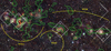 |
Fig. 1. Three-colour JHKs-band image from 2MASS of W51 (20′ × 40′), overlaid by 1.1 mm dust continuum contour from the Bolocam survey (Aguirre et al. 2011) in green and the 1.4 GHz NRAO VLA Sky Survey (NVSS, Condon et al. 1998) contours in white. The four white boxes mark the areas where photometry and spectroscopy are obtained. From left to right: field I and II cover HII region G49.5–0.4, field III G49.2–0.3 and field IV covers G48.9–0.3. The yellow arcs mark the location and extent of the 3 subregions in W51: W51A, W51B and W51C used throughout the paper. |
Exploring the larger scale picture of the W51 GMC in different tracers (Fig. 1), it becomes evident that the GMC has been fragmenting at different locations forming several star clusters 10 s of parsecs away from each other. The BOLOCAM (Aguirre et al. 2011) 1.1 mm dust continuum (green contours in Fig. 1) highlights the dense clumps in the GMC, while the 21 cm radio map from NVSS (white contours, Condon et al. 1998) shows the HII regions in the GMC. Most of the HII regions are associated with a dense mm core, suggesting that they harbour young, embedded clusters which have not yet fully evacuated the dust and gas they formed in.
To get individual measurements of each cluster and their properties, we focus on the clusters themselves. Figure 2 shows zoom-ins of the clusters in our near-infrared data obtained with SOFI, which are highlighted by white circles. In field I, there is only little diffuse emission present. The brightest star in this field is LS1 (Okumura et al. 2000), identified as a P Cygni star (Clark et al. 2009). This evolved massive star is surrounded by a diffuse shell, possibly created by its stellar wind. Field II contains the youngest region G49.5–0.4. Especially the southern region in this field shows very high extinction by dust and hosts two proto-cluster candidates (W51 Main and IRS2, Ginsburg et al. 2012). The cluster in field III seems to be emerging from the edge of a dense clump in the molecular cloud, while in field IV, we find two clusters inside the same HII region still surrounded by molecular gas.
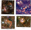 |
Fig. 2. JHKs composite colour image from the SOFI data of the 4 observed fields in W51, zoomed in on the clusters, from left to right field I, field II, field III and field IV. The red, green and blue channels are mapped to the Ks, H and J, respectively. The regions selected for the photometric analysis are indicated with white circles. The spectroscopically classified massive stars in each field are indicated with their ID numbers. In field II, also the positions of the O stars and massive YSO from Figuerêdo et al. (2008) and Barbosa et al. (2008) are shown. |
The white circles drawn in Fig. 2 highlight the sub-clusters we have selected for further analysis. The size of the white circles are chosen to cover the visual extend of the clusters and their surrounding HII region. Figure 3 shows the J–Ks vs Ks colour-magnitude diagrams (CMDs) of the different clusters. In grey scale, all the stars in the 4.9′ × 4.9′ FOV of the specific field are shown and the black points are the stars inside the drawn circles on Fig. 2. All sources with a detection in JHKs and a photometric error in all three bands less than 0.5 mag are plotted in the diagrams. The dashed line indicates the main sequence isochrone from the Geneva stellar evolution models without rotation for an age of 1 Myr (Ekström et al. 2012; Yusof et al. 2013) and assuming a distance of 5.4 kpc (Sato et al. 2010). The 1 Myr PMS isochrone of Tognelli et al. (2011) is overplotted as a solid line.
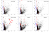 |
Fig. 3. J–Ks vs. Ks colour-magnitude diagram of the four observed fields in W51 showing the positions of all the stars in each field (grey points) and the sub-clusters (black points) defined by the circles on Fig. 2. The red triangles indicate the spectroscopically classified massive stars. The red triangle in panel b is the position of LS1 (note the different y-axis in this panel). The red squares in panel d are the massive stars classified by Figuerêdo et al. (2008) and Barbosa et al. (2008). The blue dashed vertical line represents the un-reddened isochrone for main sequence stars with an age of 1 Myr (Ekström et al. 2012; Yusof et al. 2013). The blue solid line is the reddening-free pre-main-sequence isochrone of Tognelli et al. (2011). The red lines represent the same isochrones, but reddened with AKs = 0.45 mag to highlight the foreground extinction. |
A mildly reddened, blue main sequence between J–Ks = 1 and 2 mag is visible towards all of the clusters. This is very likely the unreddened (AKs ≲ 0.45 mag) foreground population towards W51. Additionally, each panel shows a reddened cluster population starting at J–Ks ≈ 2 mag and extending to J–Ks ≈ 7 mag for the most reddened stars.
Figure 4 shows the H–Ks, J–H colour-colour diagrams (CCDs) of the same subfields. The blue dashed and solid lines represent the 1 Myr isochrone as shown in the CMD unreddened around J–H = 0 and reddened with AKs = 3.0 mag using the Nishiyama et al. (2009) extinction law around J–H = 4. The reddening line, connecting the two isochrones is plotted as a blue dashed-dotted line.
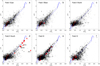 |
Fig. 4. H–Ks vs. J–H colour-colour diagram of the four observed fields in W51 showing the positions of all the stars in each field (grey points) and the sub-clusters (black points) defined by the circles in Fig. 2. The red triangles indicate the spectroscopically classified massive stars. The red triangle in panel b is the position of LS1. The red squares in panel d are the massive stars classified by Figuerêdo et al. (2008) and Barbosa et al. (2008). The blue dashed lines are the unreddened 1 Myr isochrone (around H–Ks = 0) and reddened with AKs = 3.0 mag (around H–Ks = 2.5 mag). The blue solid lines are the unreddened 1 Myr PMS isochrones and the reddened isochrone with AKs = 3.0 mag. The blue dashed-dotted is the reddening line connecting the high-mass end of the two isochrones. The red lines represent the lines at AKs = 0.45 mag. |
As in the CMD, the foreground population is clearly detected at low extinction values as a cloud of points at low J–H and H–Ks values. The cluster population is visible at higher extinction, reaching values up to AKs ≈ 3.0 mag. Apart from the spectroscopically identified OB stars it is hard to totally exclude background stars in our sample. The background stars will most likely be late type giant and AGB stars. However, by including Spitzer 8 μm observation, Nandakumar et al. (2018) showed that they can be distinguished from young and early type stars. As we are not attempting a full photometric analysis of the cluster population we do not attempt to remove the background stars, but assume the contribution is small due to the large extinction in W51.
Especially in field II, many infrared excess sources are visible as sources below the reddening line. This suggests that, together with the high extinction measured towards this region, this field contains the youngest region in our sample of clusters. A comparison between the grey and the black points shows that there are also many sources outside the white circles with a infrared excess. These are also likely member of W51, as we drew the circles on the visual extend of the clusters and HII regions, there are very likely young stars located outside the circles. Most likely the stellar population of W51 and its sub-clusters cover all the observed frames.
The photometric properties of the spectroscopically studied stars are listed in Table 3 and marked in the CMD and CCD. Additionally we add the stars of which a spectroscopic classification is done in the literature: LS1 (Clark et al. 2009) and 4 OB stars (Figuerêdo et al. 2008; Barbosa et al. 2008) to our analysis. For LS1 we used the 2MASS photometry as the source is saturated in our images. Source #12 is not detected in our J-band images, and therefore is not listed in our catalogue. For source #12 we use JHKs magnitudes from the UKIDDS Galactic Plane Survey DR6 (Lucas et al. 2008)
Spectroscopically classified OB stars in W51.
For the OB stars from Figuerêdo et al. (2008) and Barbosa et al. (2008) we matched the sources with our photometric catalogue and used our photometry. For all but one source our photometry is consistent with that of Figuerêdo et al. (2008). For W51d, however, our photometry is very different. Our J and Ks magnitudes are about a magnitude brighter than what Figuerêdo et al. (2008) found, while our H magnitude is even 2 magnitudes brighter. This results in a totally different J–H and H–Ks colour as well. Figuerêdo et al. (2008) found a large K-band excess for this source, suggesting it has a circumstellar envelope. With our photometry that Ks-band excess disappears (Fig. 4), and the source ends up close to the reddening line. The reason of the difference is not clear to us, but could be related to the very crowded and high background region this source is located in. The K-band spectrum of this source by Barbosa et al. (2008) shows a photospheric spectrum of an early O stars with He II in absorption. This would be incompatible with the spectrum of a star with a strong Ks excess as the faint He II absorption line would be invisible due to veiling by the circumstellar material. Therefore, we chose to use our photometry for the analysis of this star. The YSO IRS2E, whose spectrum is presented in Barbosa et al. (2008), is only detected in H and Ks. As our catalogues only have detections in JHKs we took its H and Ks magnitudes from Figuerêdo et al. (2008).
In Fig. 3, panel b, we show Field I where LS1 is indicated with a red triangle, however, we do no detect any other massive stars. Most spectroscopically identified OB stars are located in the southern cluster of field II. This is the location of the most active star forming complex in W51: G49.5–0.4. The OB stars from Figuerêdo et al. (2008) are shown as red squares. The location of the OB stars in the CCD (Fig. 4) shows that in field II all spectroscopically identified OB stars are highly reddened. In the two HII regions in W51B (fields III and IV) we also identify several OB stars in each region. Also in field III most OB stars in our spectroscopic sample are reddened (apart from 1 object), while in field IV, all OB stars have very low reddening. In the CCD (Fig. 4), we have two spectroscopic targets which shows a significant infrared excess. Star #16 is located in field II, south and has a H–Ks colour of 2.1 mag. With J–H = 3.08 mag this results in a mild infrared excess. The source with an extreme infrared excess is source #12.
3.2. Spectral classification
From our total spectral sample we identified 15 stars with early spectral type K-band spectra (Table 3). Their normalized K-band spectra are shown in Fig. 5. All the K-band spectra are dominated by broad Brγ in absorption. The narrow emission lines visible in several stars are due to nebular emission from the HII region. We tried to correct for the nebular contamination by fitting and subtracting the background around the positions of the spectra, but residual of the nebular emission are still present in several spectra. The spectra are not corrected for the systemic velocity of the earth, therefore some of the lines might appear shifted.
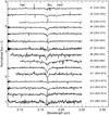 |
Fig. 5. Normalized K-band spectra of OB-type stars as taken with the multi-object mode of LUCI. The star number and their derived spectral type are indicated. Indicated with dashed lines are the diagnostic lines for the spectral classification. The narrow emission lines at 2.166 μm are of nebular origin (see text). Their profiles are truncated for clarity. |
For the earlier type stars He I (2.113 μm) and He II (2.189 μm) absorption lines are present as well as a NIII emission complex at 2.115 μm (Hanson et al. 1996, 2005). To determine the spectral types of each star, their spectra are visually compared to high resolution K-band spectra of reference OB-type stars with optical classification from Hanson et al. (2005) and Bik et al. (2005), while for spectral types mid-B and later the low-resolution spectra of Hanson et al. (1996) are used.
We performed spectral classification similar to Bik et al. (2012) as follows; high resolution, high S/N reference spectra are degraded in resolution and S/N to match the observed LUCI spectra of W51. After that a visual comparison is made between the reference spectra and the observed spectra to identify the range of best matching reference spectra and therefore best matching spectral types. The resulting spectral types are given in Table 3 and Fig. 5.
From the total sample of 15 OB stars, we identified six O stars. Three stars, #, 1, 2, and 3, are identified as early O stars, based on the lack of He I absorption and the presence of N III emission. Star #3 shows a strong contamination of Brγ emission from the HII region. This also makes the use of the He I line for the classification uncertain, as this line could be contaminated by nebular emission. We do not see any He I absorption in the spectra, suggesting a spectral type of O5V or earlier, however, the He II line is relatively weak, which suggests a spectral type as late as O8V. For this reason we classified this star as O3V–O8V. Star #3 is also included in Figuerêdo et al. (2008) as star #44 in their paper, classified as an O5V star, consistent with our classification.
The remaining nine stars are classified as B stars. Their spectral classification relies on the He I and Brγ lines, while for the late-B stars only the strength of the Brγ absorption is used as no other lines are present. Most stars show a nebular emission line on top of the Brγ absorption line. This affects the accuracy of the spectral classification, especially for the B stars where Brγ is the most important line, as we can only use the absorption wings to estimate the strength. This results in a less accurate classification which is reflected in the large uncertainty in the spectral classification.
The spectrum of star #16 shows an emission line spectrum instead of a photospheric absorption line spectrum (Fig. 6). This object shows strong Brγ emission as well as CO first-overtone emission redwards of 2.29 μm. The CO emission is seen in several (massive) YSOs and young stars with remnant accretion disks in many star forming regions (e.g. Chandler et al. 1995; Bik & Thi 2004; Blum et al. 2004; Bik et al. 2006, 2012; Puga et al. 2010; Wheelwright et al. 2010; Stolte et al. 2010; Ellerbroek et al. 2013; Ilee et al. 2013; Cooper et al. 2013; Pomohaci et al. 2017). Also the K-band spectrum of IRS2E from Barbosa et al. (2008) has a similar spectrum to that of our source #16. The CO emission originates in neutral gas with a temperature of ∼2000 K located in the inner disk (Bik & Thi 2004; Wheelwright et al. 2010). The Brγ emission line most likely originates from several different environments in the circumstellar matter such as the ionized surface of the disk, disk wind or the surrounding HII region (Bik et al. 2006). Additionally, faint Na I is detected at ∼2.208 μm consistent with warm neutral gas. This emission is detected in other YSOs as well (Cooper et al. 2013).
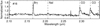 |
Fig. 6. Normalized K-band spectrum of source #16, identified as YSO based on the CO bandhead emission. The dashed lines indicate the emission lines in the spectra. |
Star #12 shows a strong near-infrared excess in the photometry, however, the K-band spectrum shows an absorption line in Brγ. This lead to the classification of B1V–B7V. The strong infrared excess from the photometry is not compatible with the K-band spectrum. Object #16 only shows a small excess in the photometry and already shows a K-band spectrum dominated by the circumstellar matter. We therefore exclude star #12 from the analysis of the HRD as the magnitudes might be affected by an infrared excess, which would result in wrong position in the HRD.
The very luminous source LS1 is also covered by our spectroscopic survey, however, the K-band spectrum is partly saturated. Spectral modelling by Clark et al. (2009) of their K-band spectrum shows that LS1 is a P Cygni type supergiant with an expanding envelope (see also Okumura et al. 2000). Clark et al. (2009) derived physical parameters for 3 different distances for LS1; 2, 3.4 and 6 kpc. They excluded the 2 kpc distance due to the fact that the derived mass would be too low to be a P Cygni supergiant. Due to the association with W51, the 6 kpc distance is favoured, bringing the mass in the more typical P Cygni supergiant regime. In the remaining of the paper we use the parameters derived for 3.4 kpc and 6 kpc (Table 4). The four O stars found by Figuerêdo et al. (2008) are all early type O stars, significantly increasing the number of spectroscopically identified O stars in W51.
Physical properties LS1.
3.3. Cluster membership
Before placing the stars in the HRD in order to compare them to evolutionary tracks, possible fore- and background stars need to be removed from the sample. The W51 complex is located rather isolated in a spiral arm with very little foreground material. The CO observations show that the W51 GMC is observed in velocity space between 50 and 70 km s−1 (e.g. Carpenter & Sanders 1998), with two additional features in the CO spectra at 7 km s−1 and between 20 and 25 km s−1. These two features are associated with foreground cloud of which the 7 km s−1 cloud is a diffuse molecular cloud and the 20−25 km s−1 mostly consist of atomic neutral hydrogen detected in absorption towards IRS2 inside W51A (Indriolo et al. 2012). No signs of active star formation has been reported for those clouds. All the HII regions are associated with the molecular material between 50 and 70 km s−1 (see for a sketch Fig. 11 of Ginsburg et al. 2015).
This makes the presence of foreground O stars rather unlikely, as they are young enough to still show part of their birth material around them. It is more likely to find foreground B stars, as they live longer and are therefore not anymore associated with molecular clouds. Foreground stars would have a much lower extinction than the cluster members as the latter are still partially embedded in the GMC. Any background source on the other hand would have a much higher extinction than the cluster members as they are behind the GMC.
As discussed in Sect. 3.1 we found five sources with very low extinction, possibly consistent with a less reddened foreground population. Source #10 is the only OB stars in field III with an AKs below 1 mag (AKs = 0.49 ± 0.04 mag), while all the other OB stars have AKs = 1.3 mag or higher. Therefore we classify source #10 as a potential foreground star. The other stars with low AKs measurements are all located in field IV (G48.9–0.3). Here all stars have consistently AKs values below 1 mag, even the early O star source #1, which is clearly located in the centre of one of the two clusters. The low extinction towards these stars could be explained by the fact that G48.9–0.3 seems to be located in front of the 68 km s−1 cloud (Ginsburg et al. 2015) instead of inside (Kang et al. 2010). Therefore we assume that all OB stars inside G48.9–0.3 are cluster members.
3.4. HRD
Using stellar atmosphere models we can derive a temperature and luminosity for each star we have spectrally classified. This allows us to compare those values to isochrones and stellar evolution tracks to derive stellar masses as well as putting constraints on the star formation history of W51. We used Martins et al. (2005) to calculate the effective temperature for the O stars. The bolometric correction and the intrinsic H–Ks colours are taken from Martins & Plez (2006). The effective temperature, bolometric correction and the intrinsic H–Ks colours of B type main sequence stars are from Pecaut & Mamajek (2013). The derived temperatures are listed in Table 5. The errors in the effective temperature are determined by the uncertainties in the spectral typing.
Physical parameters of the OB stars in W51.
With the intrinsic H–K colour we were able to derive the extinction AKs of the stars. As shown in Bik et al. (2012) and Wu et al. (2014) the choice of extinction law can have a large influence on the derived luminosity and mass, especially at very high AKs. We tested several extinction laws in the CCD to see if the slope of a given extinction law is consistent with observed reddened main sequence. The extinction laws of Román-Zúñiga et al. (2007) and Cardelli et al. (1989) are too shallow and the reddening lines are not following the reddened main sequence in the CCD. The extinction law of Fitzpatrick (1999) is too steep. The extinction laws of Rieke & Lebofsky (1985) and Indebetouw et al. (2005) are very similar in the near-infrared and provide a good fit to the reddened main sequence. The last extinction law we tested, Nishiyama et al. (2009) also provides a good fit to the data. This last extinction law is shown in the CCD, as explained in Fig. 4. Apart from the slope of the extinction, the ratio of the total over selective extinction (Rλ = Aλ/E(H − Ks)) is important when calculating the absolute extinction AKs. This cannot be constrained by JHKs data alone. In Table 5 the values for AKs listed for both the Nishiyama et al. (2009) and Indebetouw et al. (2005) extinction laws are given. The Indebetouw et al. (2005) law results in higher extinction values due to a higher RK (1.82 mag instead of 1.44 mag as in Nishiyama et al. 2009).
We derived the remaining stellar parameters for both the Indebetouw et al. (2005) and Nishiyama et al. (2009) extinction laws. The absolute K-band magnitudes were calculated by subtracting AK and the distance modulus (13.66 ± 0.12 mag) from the apparent magnitudes. Considering the bolometric correction from stellar models (Martins & Plez 2006), we derived the bolometric magnitudes and then derived the luminosity of the OB stars (Table 5). The points dereddened using the Indebetouw et al. (2005) law all have higher luminosity due to the higher extinction.
In Fig. 7 we plot the sources in the HRD together with the location of the zero age main sequence (ZAMS) from Lejeune & Schaerer (2001) as well as the 1, 2, 3 and 5 Myr isochrones (left panel) and evolutionary tracks without rotation (right panel) from Ekström et al. (2012) and Yusof et al. (2013) as well as the pre-main-sequence isochrones from Tognelli et al. (2011). For clarity we only show the HRD with the Nishiyama et al. (2009) extinction law. The HRD with de-reddening using the Indebetouw et al. (2005) extinction law is presented in Fig. B.1. The colour coding of the points in the HRD reflects the fiels in which the sources are found. The green (field III) and blue (field IV) are originating from W51B, while the red (field II) and yellow (LS1 in field I) are located in W51A.
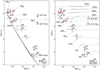 |
Fig. 7. HRD of stars identified as OB stars in our spectroscopic survey. The coloured sources are the locations with the extinction correction of Nishiyama et al. (2009). The colour coding of the sources indicates in which region they are located: red: field II, green: field III and blue: field IV. The location of LS1 (Okumura et al. 2000) for the assumed distances of 3.4 and 6 kpc is marked with a “plus” sign. The red squares are the massive stars classified by Figuerêdo et al. (2008) and Barbosa et al. (2008). Left panel: solid line represents the ZAMS isochrone from Lejeune & Schaerer (2001) and the dashed lines the main-sequence isochrones for 1, 2, 3 and 5 Myr from Ekström et al. (2012) and Yusof et al. (2013). The dash-dot lines represent the PMS isochrones of 1 and 2 Myr from Tognelli et al. (2011). Right panel: dashed lines represent the evolutionary tracks from Ekström et al. (2012) and Yusof et al. (2013). |
The masses of the stars are calculated by interpolating the tracks to the position of the stars in the HRD (Fig. 7, right panel). The errors on the masses are determined from the range of evolutionary tracks consistent with the position of the star in the HRD taking into account the error in luminosity and temperature. The resulting masses are given in Table 5 for both extinction laws. For the determination of the mass, the choice of extinction law is important and the final mass can vary a lot. For example for star #3 the masses we derive differ by a factor 2 from each other (100 vs. 200 M⊙). The final column of Table 5 provides the average of the masses derived for the two extinction laws.
Also the O stars from Figuerêdo et al. (2008) and Barbosa et al. (2008) are included in the HRD. We use the spectral types and the magnitudes in Table 3 and calculate their luminosity, effective temperature and mass in the same way as the other stars. As for most of these stars no range in spectral types is given, we plot the position without error bar. Also LS1 is added to the HRD, where the luminosity and effective temperature are taken from Table 4.
For sources #1, #2, #3 and W51d, the left error bar is plotted as an arrow. The reason for this is that the spectral type corresponding to that error bar is O3V (log Teff = 4.652), which is the earliest spectral type listed in the tables of Martins et al. (2005) and with existing near-infrared classification criteria (Hanson et al. 2005). This means that in our HRD there are no points to the left of log Teff = 4.652, making the upper temperature error of these stars in a lower limit. Stars hotter than log Teff = 4.652 will be classified as O3V star with the current near-infrared classification. This degeneracy can be solved by spectral fitting with stellar atmosphere models.
Our sample includes stars from early type O stars, down to late B-early A stars, spanning five orders of magnitude in luminosity in the HRD. We identify eight stars of early and mid-O spectral type with masses above 30 M⊙ in the W51 GMC, of which most are located in the G49.5–0.4 HII region (field II).
The sources with late O to early B spectral types (#4, 6, 7 and 12) are located a bit above the main sequence, however, all within 2 sigma away from the stellar isochrones. Sources #13 and 14 are located even further from the main sequence isochrones. Source #15 is consistent with being a 1–2 Myr old pre-main-sequence star. We discuss this displacement in detail in Sect. 4.1.
3.5. Energy budget HII regions
The W51 GMC harbours numerous HII regions, each ionized by one or more massive stars. The radio free-free emission observed from these HII regions can be used as a proxy for the spectral type of the ionizing sources. Most of the radio observations have been focussed on the most active site of star formation: the W51A cloud. Mehringer (1994) performed high resolution VLA observations with a spatial resolution of 3.1″ at 3.6 cm of the W51A cloud and covered our fields II and III. Ginsburg et al. (2012) zoomed in the central part of W51A and presented observations with a spatial resolution of 0.3″ at 2 and 6 cm.
We compared the location of the spectroscopically identified OB stars with these radio observations and found for five stars in field II the corresponding HII region (Table 6). Additionally, the clusters in field III and IV have their own H II region and we only list their most massive stars as they are the dominant source of ionizing photons.
HII regions associated with massive stars.
When comparing the spectral types derived from the radio free-free emission with that of the stars inside the HII regions, we found in most cases good agreement, thus confirming that we have identified the main ionizing sources of those regions. In two regions (G49.5–0.4 c1 and e7) we find that the radio spectral type is significantly earlier than the spectrum of the star inside the HII region. This suggests that another massive stars, possibly more deeply embedded in this HII region, is responsible for its ionization.
The dust cocoons around several of these HII regions are also detected in the mid-infrared imaging of Lim & De Buizer (2019), suggesting that these HII regions harbour very young objects. HII region e7 around star #7 is even identified as a massive YSO candidate. The other HII regions are more extended, possible suggesting a slightly more evolved nature.
Also, there are many O stars without identified HII region and vice versa. This is because of two reasons. The radio emission in this area is very complex and due to confusion as well as the fact that radio interferometers typically are sensitive to a limited range in spatial scales, it might well be that some of the fainter HII regions are missed. Our spectroscopic census is not complete and several bright point sources have not been observed, therefore it is very likely that we missed some O stars.
4. Discussion
We obtained K-band spectroscopy and near-infrared imaging of members of four HII regions in the W51 GMC complex. Below we discuss the implications of our findings for our understanding of the star formation history for each individual region and W51 as a whole. Table 7 summarizes the basic properties of the four observed clusters.
Properties of different HII regions and their massive stellar content.
4.1. Age of the stellar population
We can compare the position of the massive stars in W51 in the HRD (Fig. 7) with the location of the theoretical isochrones and derive constraints on the age of the stellar population. The early O stars, sources #1, 2, W51d, 57 and 3 are all located between the ZAMS and the 2 Myr isochrones. Sources #5, 50 and 61 are a bit to the right of the 2 Myr isochrone and, especially 61, more consistent with the 3 Myr track.
However, several of these stars have a very high extinction and a change of extinction law changes their position in the HRD significantly. Comparing the HRD made with the Nishiyama et al. (2009) extinction law (Fig. 7) with the diagram created with the Indebetouw et al. (2005) extinction law (Fig. B.1), the position of #5, 60 and 61 all move upward and become more consistent with the 2 Myr isochrone.
The sources with late B to early A spectral types overlap in the HRD with the PMS tracks and can also be used to constrain the age of the stellar population. Sources #8 and #15 would be classified as intermediate mass pre-main-sequence stars with an age of 1–2 Myr, consistent with the age found for the massive stars. Source #10 was classified as foreground star due to it’s very low extinction compared to the other stars in Field III.
We have detected 3 early-mid B stars in W51 (#4,#6, #7 ) as well as 2 late B stars (#13 and #14) whose location in the HRD (for both extinction laws) is not consistent with the above derived age of 1–3 Myr. Sources #4, #6 and #7 are 1.5–2σ away from the 1–3 Myr isochrones, while sources 13 and 14 are more than 3σ away. Also in other star forming regions we found that the B stars are not matching with the same isochrones as the O stars (Bik et al. 2012; Wu et al. 2016). From all the 5 sources, only 1 source (#13) is located slightly to the right of the reddening line in the CCD (Fig. 4), suggesting that it has as small colour excess (∼0.25 mag in (H − K). However, this would only result in a 25% increase in luminosity, not explaining the large offset of source #13 from the isochrones.
The classification of the B stars relies on just one (late B) or two (early- mid B) absorption lines (Hanson et al. 1996). This is reflected in the large error bars of the stars in the HRD, however, cannot explain the large offset. For sources #4, 6 and 7 the observed luminosity is consistent with them being late O stars, this is however not compatible with just the detection of Brγ and He I.
In Bik et al. (2012) several possibilities are listed causing a displacement in the HRD. It has become clear that most massive stars are observed as binaries (e.g. Apai et al. 2007; Sana et al. 2012, 2017; Ramírez-Tannus et al. 2017). The combined luminosity would be a factor 2 higher in the case of an equal mass binary, again only explaining part of large offset in luminosity observed. Another possibility is that the stars are not part of W51, but are located in the foreground. Sources #6 and #7 are associated with radio sources c1 and e7 (see Sect. 3.5). Additionally, the measured foreground extinction towards all the sources is similar to the other stars in W51. As shown in Sect. 3.3 there is very little molecular material along the line of sight towards W51 and non of that is associated with star formation. This makes the stars most likely member of W51.
The other possibility is that the B stars are in a different evolutionary state than the O stars. Stars #4 and #6 overlap within their error bars with the 5 Myr isochrone. This would make their age consistent with LS1. Alternatively, these stars could be massive pre-main-sequence stars. Theoretical simulations of massive stars predict the presence of massive PMS stars (e.g Hosokawa & Omukai 2009). Deep optical and near-infrared studies of high-mass star forming regions have revealed several candidates for this evolutionary phase (Ochsendorf et al. 2011; Bik et al. 2012; Ramírez-Tannus et al. 2017). Especially, sources #6 and #7 could be good candidates, as they are surrounded by a compact HII region, still embedded in their natal dust cocoon, suggesting they are young objects. Follow-up optical spectra would allow a better spectral classification as well as a determination of their surface gravity. These observations would provide more constraints on their evolutionary state.
The black plus signs show the location of LS1 assuming a distance of 3.4 and 6 kpc distance, where the parameters are taken from Clark et al. (2009) and listed in Table 4. The position in the HRD made Clark et al. (2009) conclude that LS1 is at least 3 Myr old, with a likely age between 3 and 6 Myr for the furthest distance. This would suggest an age difference between LS1 and the O type stars in W51 and therefore an extended star formation history (Clark et al. 2009). No directed search has been done in W51 to identify the lower-mass stars formed in the same star formation epoch as LS1. The spatially variable extinction and diffuse emission makes it hard to obtain accurate ages with only photometric data. Some of the observed B stars above the isochrones could be part of this population, even though the B stars are not located in the same field as LS1 (Field I), but in fields II and III.
We know from the longer wavelength observations that currently star formation is still active, especially in the W51A cloud (Ginsburg et al. 2015). In G49.5–04 two proto clusters are still forming (Ginsburg et al. 2012). In the near-infrared we are sensitive to find stars with an age of a few Myr, while at mm wavelength, where extinction is not an issue, much younger objects can be identified. However, the near-infrared traces the only spectral window to directly detect and characterize the photosphere of the most recently formed OB stars.
Concluding, we found a very young massive star population consistent with an age of 3 Myr or less. Other epochs of star formation in W51 are found via mm observations (the ongoing star formation) and the identification of LS1, an evolved massive star. The evolutionary state of some of the B stars remains inconclusive as they could belong to either older or the very young stellar population.
4.2. Cluster properties
The properties of the clusters inside the HII regions where we have identified OB stars are summarised in Table 7. The molecular masses are derived based on CO observations by Kang et al. (2010) for the W51A cloud and by Carpenter & Sanders (1998) for the HII regions in W51B. The stellar masses are estimated by Okumura et al. (2000, W51a) and Nanda Kumar et al. (2004, W51B) based on near-infrared photometry. Okumura et al. (2000) derived a slope of the IMF of 1.8 (with Salpeter being 1.3), based on the more massive stars, which they extrapolated to lower masses to derive the total cluster mass. Nanda Kumar et al. (2004) derived their cluster masses using the procedure outlined in Lada & Lada (2003) making use of the K-band luminosity function.
Based on the masses of the spectroscopically identified OB stars we can get an independent estimate of the cluster mass. We assumed a Kroupa (2002) IMF and used the number of stars (eight) with photometric masses between 37 and 120 M⊙ identified by us in the W51 cloud as boundary condition. We carried out Monte Carlo simulations by randomly drawing a population from the IMF as described in Brandner et al. (2008). Based on this we derived a most likely cluster mass of 5 × 10³M⊙, a factor of ten lower than the literature value based on near-infrared imaging (Okumura et al. 2000; Nanda Kumar et al. 2004). This difference shows how much we are incomplete in sampling the high-mass stellar population. As can be seen the in CMD (Fig. 3) and CCD (Fig. 4) of W51, there are many bright, reddened point sources from which we do not have near-infrared spectra. Even the near-infrared photometry mass estimate is likely still a lower limit, especially in the very extincted regions like G49.5–0.4.
Once we know the molecular and stellar masses we can estimate the star formation efficiency (SFE). Using the cluster masses from Okumura et al. (2000) and Nanda Kumar et al. (2004) and the molecular mass of Carpenter & Sanders (1998) we derive a SFE of 3% for the entire W51 complex. This is similar to what is found on GMC scales in the Milky Way as well as other galaxies (e.g. Murray 2011; Kennicutt & Evans 2012). Based on the YSOs detected in Spitzer images, Kang et al. (2009, 2010) derived a SFE of ∼1% for the entire W51 region.
When we zoom in to the individual HII regions, we find much higher SFEs. For G49.5–0.4 (our field II) a SFE of 17% is found based on the near-infrared data of Kang et al. (2010) and the molecular observations of Carpenter & Sanders (1998). This is likely still even a lower limit as the stellar population is so reddened that even in the near-infrared a large fraction will be missed. In fact, all the spectroscopically detected O stars in G49.5–0.4 have AKs > 2.5 mag. For the two regions in W51B we find 17% for G49.2–0.3 (field III) and even 35% for G48.9–0.3 (field IV). Derivation of SFEs towards the denser cores of GMCs in which the clusters are forming are generally much higher than SFEs averaged over an entire GMC. Simulations predict that the gravitationally bound regions of the clouds form star clusters with a higher SFE than the more dispersed population formed in unbound regions of the molecular clouds (Bonnell et al. 2011). Similar results have been found in starburst region W43 where the SFE increases with increasing density of H2 (Louvet et al. 2014).
On the other hand, gas dispersion due to stellar feedback can also result in a measured high star formation efficiency. Ginsburg et al. (2015) shows that in W51B the star formation has mostly stopped and there is little dense gas left. The feedback of the massive stars in these two clusters is now dispersing and/or ionizing the cloud. This could be the reason for the high SFE in G48.9–0.3, where already a significant fraction of the molecular material is removed. The cluster contains an early O star (#1) and the ionizing photons and stellar wind emitted by the star is efficient in removing, especially, the low-density molecular gas (Dale et al. 2013).
4.3. Spatial distribution of the massive stars in GMC region
Using Fig. 2 we can look at the spatial distribution of the (massive) stars and compare this to other star-forming complexes in the literature and relate the spatial distribution to the formation mechanisms of OB associations and star clusters. The W51 GMC contains many clusters spatially separated from each other, each surrounded by their own HII region (e.g. G48.9–0.3 and G49.2–0.3). When we compare the location of the spectroscopically identified massive stars we find that not all the massive stars are located inside the clusters. In both G48.9–0.3 and G49.2–0.3 we found massive stars in the central region, however, there are also several B stars dispersed around the cluster. (#8 in G48.9–0.2 and #4, #14 and #15 in G49.3–0.4, Fig. 2). In these regions, at least the massive stars are located where the diffuse emission (Brγ) from the HII region is located. The B stars do not emit enough ionizing photons to create a detectable HII region.
Most massive stars in our sample are located in G49.5–0.4 (field II), the most massive region in W51. Figure 2 panel III shows their spatial distribution. We found only few O stars associated with the currently forming proto-clusters associated with the HII regions W51d and W51e. These stars (W51d and IRS2E) are very deeply embedded and we clearly miss a large fraction of the stars forming there. We also found several of the spectroscopically identified massive stars outside these two clusters. Some of the O stars we detected (#6, #7) are associated with diffuse emission likely caused by Brγ emission from a small HII region (see also Sect. 3.5). Similar results have been found for the youngest massive stars in W51, where Saral et al. (2017) found that most massive YSOs are associated with HII regions. However, we also find sources not associated with HII regions: sources 57 and 61 from Figuerêdo et al. (2008) are not (anymore) associated with any HII regions, but are among the most massive stars detected in this region (Table 5).
The observation that not all massive stars in G49.5–0.4 are part of the two forming proto-clusters can be explained by two scenarios. First, the stars outside the cluster can be run-away stars (Blaauw 1961), where the star is ejected out of the star cluster by the supernova explosion of the binary companion or via dynamical interactions in the cluster (e.g. Gvaramadze et al. 2009). Taking a typical velocity of 100 km s−1 (Gvaramadze et al. 2010) and assuming an age of 2 Myr would result at a displacement of ∼200 pc away from the birthplace. This distance is larger than the size of the W51 GMC, indicating that these stars could be runaway stars. As the stars are still very young, the supernova kick scenario would be unlikely. In the dynamical ejection scenario, the less massive star involved in the dynamical three- or four body interaction is expelled (e.g. Gvaramadze et al. 2009). The two stars 57 and 61 are among the most massive stars in W51, making also this scenario not very likely.
The other explanation is that massive stars do not exclusively form in the highest density regions of the GMC where the proto-clusters are forming, but also in their immediate surroundings. Observations of other large star forming sites such as G305 (Davies et al. 2012), the Carina region (Smith 2006; Feigelson et al. 2011) and 30 Doradus (Bressert et al. 2012) showed similar behaviour. These regions contain dense star clusters but also a spatially extended O star population. In W49 we found that massive stars are more centrally concentrated around the main cluster (Wu et al. 2016), however also there we identified several stars outside the central cluster.
This spatial distribution can be related to the properties of the GMCs in which the stars have formed. GMCs do not have a smooth density distribution, but are highly turbulent resulting in a hierarchical distribution of densities. Modelling by Bonnell et al. (2011) shows that the densest, gravitationally bound regions in the GMCs could give rise to gravitationally bound stellar clusters formed with a high star formation efficiency, while in the unbound parts of the clouds a more spatially dispersed population forms.
4.4. Star formation history
The different stellar populations discussed in this paper and many other studies, show that W51 has a complex star forming history. We find a population of massive OB stars with an estimated age of 3 Myr or less. The presence of the evolved P Cygni-type supergiant suggests that star formation at some rate has been going on for longer than 3 Myr (Okumura et al. 2000; Clark et al. 2009). Additionally, in the centre of W51A, two proto-clusters (Ginsburg et al. 2012) are located which are currently forming stars on a very high rate. This raises the question how the star formation was initiated and how it proceeds. Due to the large extend and elongated shape of the W51 GMC several authors suggested, or could not exclude the possibility, that an external triggering mechanism working on large scales, such as a spiral arm passage is responsible for the star formation (Koo 1999; Nanda Kumar et al. 2004; Clark et al. 2009).
On the presence of smaller scale triggering, however, the opinions highly vary. Koo & Moon (1997) found evidence for the presence of shockwaves in the interface between the supernova remnant W51C and the GMC from HI and X-ray observations, suggesting that the supernova has affected the molecular cloud. However, considering the estimated age of the supernova remnant W51C of only 30 kyr (Koo et al. 1995), the formation of the stars we observed in G49.2–0.3, the HII region closest to W51C, could not be triggered by the supernova event. This is supported by the lack of dense gas showing that the collect-and-collapse scenario is not at play in this region (Ginsburg et al. 2015).
Sequential star formation in G49.5–0.4 was proposed by Okumura et al. (2000). By investigating their NIR photometry, an age spread between their regions 1, 2 and 3 has been found, implying the internal triggered star formation from north to south. Clark et al. (2009) object against this hypothesis because if region 1 triggered similar star formation activity in region 3, then we might expect to see a large wind blown cavity in mid-IR created by stars like LS1 in region 1. But Spitzer observations reveal that IRS2 does not resides on the boundaries of any wind bubble, implying IRS2 formed independently of the effect of other regions. Additionally, evidence for cloud-cloud collisions inside G49.5–0.4 has been presented by Kang et al. (2010) and Fujita et al. (2017).
Based on our spectroscopy in combination with the other literature data we can derive a relative time line for the four regions we have studied in detail. The HII region in field I, G49.58–0.038 contains little dust and ionized gas as traced by the green and white contours in Fig. 1. This suggests that this region is one of the older regions in W51 as most of the gas and dust have been dispersed. Additionally, towards this region we observe also the evolved star LS1. Under the assumption that this star is associated with the HII region, this would place an age estimate of 3–6 Myr (Clark et al. 2009) on this region.
For the other regions, the HRD analysis shows that they all have an age younger than ∼3 Myr. However, based on additional, more indirect arguments we can still derive a relative sequence. The youngest of the regions is vey likely G49.5–0.4 (field II), because of its high gas density and the presence of two proto-clusters. The extinction towards the massive stars in this region is the highest of all 4 regions studied.
From the two regions in W51B, G48.9–0.3 (field IV) is likely older than G49.2–0.3 (field III). The OB stars identified in G48.9–0.3 have the lowest extinction of all the four regions, suggesting that the cluster has cleared out most of the dust. Additionally, the amount of molecular material around this cluster is also relatively low, resulting in the very high SFE derived for this region (Sect. 4.2). The cluster is already relatively evolved and has dispersed a large fraction of its parental molecular cloud. This results in an evolutionary sequence (see Fig. 8) with G49.58–0.038 being the oldest, after that G48.9–0.3 formed, then G49.2–0.3, and finally G49.5–0.4, which is currently still forming stars at a high rate.
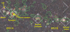 |
Fig. 8. Three-colour image of W51 (identical to Fig. 1) overlayed with the annotation of the evolutionary state of the different clusters discussed in Sect. 4.4 as well as the location of the two proto clusters identified in Ginsburg et al. (2012) and the evolved massive star LS1. |
Their spatial distribution excludes the triggering scenario proposed by Okumura et al. (2000) as the two oldest regions are at the two extreme ends of the molecular cloud. This sequence confirms the conclusions of Clark et al. (2009), suggesting that star formation in W51 is a multi-seeded process where molecular clumps in the W51 GMC collapse at slightly different times resulting in the observed star formation. In the densest regions, like G49.5–0.4 internal triggering likely plays a role in the formation of some of the stars, but overall, triggering is not the dominant mode of star formation in W51.
Recent kinematic studies of OB associations showed that they are not expanding clusters (e.g. Baumgardt & Kroupa 2007), but are made of kinematically independent sub-structure. They consist of the product of low-density multi-seeded star formation where each of the sub-clusters leaves their own kinematic signature (Wright et al. 2016; Wright & Mamajek 2018; Ward & Kruijssen 2018; Kuhn et al. 2019). The observed properties of W51 show that W51 is also such an OB association, where we currently witness several of the sub-clusters being formed, while others are already slightly more evolved.
5. Conclusions
In this paper, we presented JHKs imaging from NTT/SOFI and K-band spectroscopy from LBT/LUCI of the stellar content in the star-forming region of W51. We derived the following results and conclusions on the W51 GMC:
-
1.
We constructed CMDs and CCDs of four fields for which we collected near-infared imaging and spectroscopic data. We found that the locations of the OB stars in the CCD are consistent with reddened photospheres. Additionally, we found several sources showing an infrared excess, suggesting the presence of sources with circumstellar disks in W51. We found a range of extinctions, with the youngest region. G49.5–0.4 (field II) showing the highest values. G48.9–0.3 (field IV) shows very low extinction, suggesting that this region is already more evolved.
-
2.
We identified 15 O and B stars based on their absorption line spectra and one source with a circumstellar disk showing CO bandhead emission. The most massive star discovered by our spectroscopic survey is star #3 (with an estimated mass of ∼100 M⊙). We added four O stars identified in the literature and derived the age of the stellar population to be consistent with ∼3 Myr or less.
-
3.
We analysed the properties of the clusters in which we have identified OB stars and found star-formation efficiencies higher than the overall SFE of W51 (1–3%). This is consistent to what is observed towards other GMCs. The more evolved cluster (G48.9–0.3) shows a very high apparent SFE (35%). The SFE at the time of formation might have been substantially lower as the majority of the gas is already expelled from the cluster.
-
4.
Finally we did not find evidence for triggered star formation being the dominant mode of star formation in W51. We did not find a progressive age-space sequence in the GMC, as the two regions on the northern (field I) and southern end (field IV) seem to be the most evolved regions. We support the conclusions drawn in the literature that star formation in W51 is multi-seeded. We conclude that W51 is an OB association.
The UKIDSS project is defined in Lawrence et al. (2007). UKIDSS uses the UKIRT Wide Field Camera (WFCAM; Casali et al. 2007) and a photometric system described in Hewett et al. (2006). The pipeline processing and science archive are described in Irwin (2008) and Hambly et al. (2008). We have used data from the 7th data release, which is described in detail in Warren et al. (2007).
Acknowledgments
We thank the referee for the comments and suggestions which improved the paper. We thank Kate Rubin, Jaron Kurk and Barry Rothberg for carrying out part of the observations. A.B. acknowledges MPIA for hospitality and travel support. A.P. acknowledges support from Sonderforschungsbereich SFB 881 “The Milky Way System” (subproject B5) of the German Research Foundation (DFG). Based on data obtained from the ESO Science Archive Facility. This research has made use of NASA’s Astrophysics Data System Bibliographic Services (ADS). This research has made use of the SIMBAD database, operated at CDS, Strasbourg, France (Wenger et al. 2000). IRAF is distributed by the National Optical Astronomy Observatory, which is operated by the Associated Universities for Research in Astronomy, Inc., under cooperative agreement with the National Science Foundation.
References
- Ageorges, N., Seifert, W., Jütte, M., et al. 2010, Proc. SPIE, 7735, 53 [NASA ADS] [Google Scholar]
- Aguirre, J. E., Ginsburg, A. G., Dunham, M. K., et al. 2011, ApJS, 192, 4 [NASA ADS] [CrossRef] [MathSciNet] [Google Scholar]
- Aleksić, J., Alvarez, E. A., Antonelli, L. A., et al. 2012, A&A, 541, A13 [NASA ADS] [CrossRef] [EDP Sciences] [Google Scholar]
- Apai, D., Bik, A., Kaper, L., Henning, T., & Zinnecker, H. 2007, ApJ, 655, 484 [NASA ADS] [CrossRef] [Google Scholar]
- Ascenso, J., Alves, J., Beletsky, Y., & Lago, M. T. V. T. 2007, A&A, 466, 137 [NASA ADS] [CrossRef] [EDP Sciences] [Google Scholar]
- Bally, J. 2008, in Handbook of Star Forming Regions, ed. B. Reipurth, ASP Conf., 4, 459 [NASA ADS] [Google Scholar]
- Barbosa, C. L., Blum, R. D., Conti, P. S., Damineli, A., & Figuerêdo, E. 2008, ApJ, 678, L55 [NASA ADS] [CrossRef] [Google Scholar]
- Baumgardt, H., & Kroupa, P. 2007, MNRAS, 380, 1589 [NASA ADS] [CrossRef] [Google Scholar]
- Beccari, G., Spezzi, L., De Marchi, G., et al. 2010, ApJ, 720, 1108 [NASA ADS] [CrossRef] [Google Scholar]
- Berlanas, S. R., Herrero, A., Comerón, F., et al. 2018, A&A, 612, A50 [NASA ADS] [CrossRef] [EDP Sciences] [Google Scholar]
- Bik, A., & Thi, W.-F. 2004, A&A, 427, L13 [NASA ADS] [CrossRef] [EDP Sciences] [Google Scholar]
- Bik, A., Kaper, L., Hanson, M. M., & Smits, M. 2005, A&A, 440, 121 [NASA ADS] [CrossRef] [EDP Sciences] [Google Scholar]
- Bik, A., Kaper, L., & Waters, L. B. F. M. 2006, A&A, 455, 561 [NASA ADS] [CrossRef] [EDP Sciences] [Google Scholar]
- Bik, A., Puga, E., Waters, L. B. F. M., et al. 2010, ApJ, 713, 883 [NASA ADS] [CrossRef] [Google Scholar]
- Bik, A., Henning, T., Stolte, A., et al. 2012, ApJ, 744, 87 [NASA ADS] [CrossRef] [Google Scholar]
- Bik, A., Stolte, A., Gennaro, M., et al. 2014, A&A, 561, A12 [Google Scholar]
- Blaauw, A. 1961, Bull. Astron. Inst. Neth., 15, 265 [Google Scholar]
- Blaauw, A. 1991, NATO ASIC Proc. 342: The Physics of Star Formation and Early Stellar Evolution, 1, 125 [NASA ADS] [CrossRef] [Google Scholar]
- Blum, R. D., Barbosa, C. L., Damineli, A., Conti, P. S., & Ridgway, S. T. 2004, ApJ, 617, 1167 [NASA ADS] [CrossRef] [Google Scholar]
- Bonnell, I. A., Smith, R. J., Clark, P. C., & Bate, M. R. 2011, MNRAS, 410, 2339 [NASA ADS] [CrossRef] [Google Scholar]
- Brandner, W., Clark, J. S., Stolte, A., et al. 2008, A&A, 478, 137 [NASA ADS] [CrossRef] [EDP Sciences] [Google Scholar]
- Bressert, E., Bastian, N., Evans, C. J., et al. 2012, A&A, 542, A49 [NASA ADS] [CrossRef] [EDP Sciences] [Google Scholar]
- Brogan, C. L., Goss, W. M., Hunter, T. R., et al. 2013, ApJ, 771, 91 [NASA ADS] [CrossRef] [Google Scholar]
- Brown, A. G. A., de Geus, E. J., & de Zeeuw, P. T. 1994, A&A, 289, 101 [NASA ADS] [Google Scholar]
- Buschkamp, P., Hofmann, R., Gemperlein, H., et al. 2010, Proc. SPIE, 7735, 236 [NASA ADS] [Google Scholar]
- Cardelli, J. A., Clayton, G. C., & Mathis, J. S. 1989, ApJ, 345, 245 [NASA ADS] [CrossRef] [Google Scholar]
- Carpenter, J. M., & Sanders, D. B. 1998, AJ, 116, 1856 [NASA ADS] [CrossRef] [Google Scholar]
- Casali, M., Adamson, A., Alves de Oliveira, C., et al. 2007, A&A, 467, 777 [NASA ADS] [CrossRef] [EDP Sciences] [Google Scholar]
- Chandler, C. J., Carlstrom, J. E., & Scoville, N. Z. 1995, ApJ, 446, 793 [NASA ADS] [CrossRef] [Google Scholar]
- Clark, J. S., Negueruela, I., Crowther, P. A., & Goodwin, S. P. 2005, A&A, 434, 949 [NASA ADS] [CrossRef] [EDP Sciences] [Google Scholar]
- Clark, J. S., Davies, B., Najarro, F., et al. 2009, A&A, 504, 429 [NASA ADS] [CrossRef] [EDP Sciences] [Google Scholar]
- Comerón, F., & Pasquali, A. 2012, A&A, 543, A101 [NASA ADS] [CrossRef] [EDP Sciences] [Google Scholar]
- Comerón, F., Pasquali, A., Rodighiero, G., et al. 2002, A&A, 389, 874 [NASA ADS] [CrossRef] [EDP Sciences] [Google Scholar]
- Condon, J. J., Cotton, W. D., Greisen, E. W., et al. 1998, AJ, 115, 1693 [NASA ADS] [CrossRef] [Google Scholar]
- Cooper, H. D. B., Lumsden, S. L., Oudmaijer, R. D., et al. 2013, MNRAS, 430, 1125 [NASA ADS] [CrossRef] [Google Scholar]
- Da Rio, N., Robberto, M., Soderblom, D. R., et al. 2010, ApJ, 722, 1092 [NASA ADS] [CrossRef] [Google Scholar]
- Dale, J. E., Ngoumou, J., Ercolano, B., & Bonnell, I. A. 2013, MNRAS, 436, 3430 [NASA ADS] [CrossRef] [Google Scholar]
- Davies, R. I. 2007, MNRAS, 375, 1099 [NASA ADS] [CrossRef] [Google Scholar]
- Davies, B., Clark, J. S., Trombley, C., et al. 2012, MNRAS, 419, 1871 [NASA ADS] [CrossRef] [Google Scholar]
- de Zeeuw, P. T., Hoogerwerf, R., de Bruijne, J. H. J., Brown, A. G. A., & Blaauw, A. 1999, AJ, 117, 354 [NASA ADS] [CrossRef] [Google Scholar]
- Devillard, N. 2001, in Astronomical Data Analysis Software and Systems X, eds. F. R. Harnden, F. A. Primini, & H. E. Payne, ASP Conf. Ser., 238, 525 [NASA ADS] [Google Scholar]
- Eden, D. J., Moore, T. J. T., Urquhart, J. S., et al. 2018, MNRAS, 477, 3369 [NASA ADS] [CrossRef] [Google Scholar]
- Ekström, S., Georgy, C., Eggenberger, P., et al. 2012, A&A, 537, A146 [NASA ADS] [CrossRef] [EDP Sciences] [Google Scholar]
- Ellerbroek, L. E., Bik, A., Kaper, L., et al. 2013, A&A, 558, A102 [NASA ADS] [CrossRef] [EDP Sciences] [Google Scholar]
- Elmegreen, B. G. 2000, ApJ, 530, 277 [NASA ADS] [CrossRef] [Google Scholar]
- Elmegreen, B. G. 2008, ApJ, 672, 1006 [NASA ADS] [CrossRef] [Google Scholar]
- Elmegreen, B. G. 2009, Proc. Int. Astron. Union, 5, 3 [CrossRef] [Google Scholar]
- Feigelson, E. D., & Townsley, L. K. 2008, ApJ, 673, 354 [NASA ADS] [CrossRef] [Google Scholar]
- Feigelson, E. D., Getman, K. V., Townsley, L. K., et al. 2011, ApJS, 194, 9 [NASA ADS] [CrossRef] [Google Scholar]
- Feigelson, E. D., Townsley, L. K., Broos, P. S., et al. 2013, ApJS, 209, 26 [Google Scholar]
- Figuerêdo, E., Blum, R. D., Damineli, A., Conti, P. S., & Barbosa, C. L. 2008, AJ, 136, 221 [NASA ADS] [CrossRef] [Google Scholar]
- Fitzpatrick, E. L. 1999, PASP, 111, 63 [NASA ADS] [CrossRef] [Google Scholar]
- Fujita, S., Torii, K., Kuno, N., et al. 2017, ArXiv e-prints [arXiv:1711.01695] [Google Scholar]
- Gaia Collaboration (Prusti, T., et al.) 2016, A&A, 595, A1 [NASA ADS] [CrossRef] [EDP Sciences] [Google Scholar]
- Gennaro, M., Brandner, W., Stolte, A., & Henning, T. 2011, MNRAS, 412, 2469 [NASA ADS] [CrossRef] [MathSciNet] [Google Scholar]
- Gennaro, M., Bik, A., Brandner, W., et al. 2012, A&A, 542, A74 [NASA ADS] [CrossRef] [EDP Sciences] [Google Scholar]
- Ginsburg, A. 2017, Star Formation Newsletter #290 [Google Scholar]
- Ginsburg, A., Bressert, E., Bally, J., & Battersby, C. 2012, ApJ, 758, L29 [NASA ADS] [CrossRef] [Google Scholar]
- Ginsburg, A., Bally, J., Battersby, C., et al. 2015, A&A, 573, A106 [NASA ADS] [CrossRef] [EDP Sciences] [Google Scholar]
- Ginsburg, A., Goss, W. M., Goddi, C., et al. 2016, A&A, 595, A27 [NASA ADS] [CrossRef] [EDP Sciences] [Google Scholar]
- Ginsburg, A., Goddi, C., Kruijssen, J. M. D., et al. 2017, ApJ, 842, 92 [Google Scholar]
- Goldader, J. D., & Wynn-Williams, C. G. 1994, ApJ, 433, 164 [NASA ADS] [CrossRef] [Google Scholar]
- Gvaramadze, V. V., Gualandris, A., & Portegies Zwart, S. 2009, MNRAS, 396, 570 [NASA ADS] [CrossRef] [Google Scholar]
- Gvaramadze, V. V., Kroupa, P., & Pflamm-Altenburg, J. 2010, A&A, 519, A33 [NASA ADS] [CrossRef] [EDP Sciences] [Google Scholar]
- Hambly, N. C., Collins, R. S., Cross, N. J. G., et al. 2008, MNRAS, 384, 637 [NASA ADS] [CrossRef] [Google Scholar]
- Hanson, M. M., Conti, P. S., & Rieke, M. J. 1996, ApJS, 107, 281 [Google Scholar]
- Hanson, M. M., Kudritzki, R.-P., Kenworthy, M. A., Puls, J., & Tokunaga, A. T. 2005, ApJS, 161, 154 [NASA ADS] [CrossRef] [EDP Sciences] [MathSciNet] [Google Scholar]
- Harfst, S., Portegies Zwart, S., & Stolte, A. 2010, MNRAS, 409, 628 [NASA ADS] [CrossRef] [Google Scholar]
- Hewett, P. C., Warren, S. J., Leggett, S. K., & Hodgkin, S. T. 2006, MNRAS, 367, 454 [NASA ADS] [CrossRef] [Google Scholar]
- Hill, J. M., Green, R. F., & Slagle, J. H. 2006, Proc. SPIE, 6267, 31 [NASA ADS] [Google Scholar]
- Hosokawa, T., & Omukai, K. 2009, ApJ, 691, 823 [NASA ADS] [CrossRef] [Google Scholar]
- Hussmann, B., Stolte, A., Brandner, W., Gennaro, M., & Liermann, A. 2012, A&A, 540, A57 [NASA ADS] [CrossRef] [EDP Sciences] [Google Scholar]
- Ilee, J. D., Wheelwright, H. E., Oudmaijer, R. D., et al. 2013, MNRAS, 429, 2960 [NASA ADS] [CrossRef] [Google Scholar]
- Indebetouw, R., Mathis, J. S., Babler, B. L., et al. 2005, ApJ, 619, 931 [NASA ADS] [CrossRef] [Google Scholar]
- Indriolo, N., Neufeld, D. A., Gerin, M., et al. 2012, ApJ, 758, 83 [NASA ADS] [CrossRef] [Google Scholar]
- Irwin, M. J. 2008, The 2007 ESO Instrument Calibration Workshop (Berlin, Heidelberg: Springer, Berlin Heidelberg), 541 [Google Scholar]
- Kang, M., Bieging, J. H., Povich, M. S., & Lee, Y. 2009, ApJ, 706, 83 [NASA ADS] [CrossRef] [Google Scholar]
- Kang, M., Bieging, J. H., Kulesa, C. A., et al. 2010, ApJS, 190, 58 [NASA ADS] [CrossRef] [Google Scholar]
- Kausch, W., Noll, S., Smette, A., et al. 2015, A&A, 576, A78 [NASA ADS] [CrossRef] [EDP Sciences] [Google Scholar]
- Kennicutt, R. C., & Evans, N. J. 2012, ARA&A, 50, 531 [NASA ADS] [CrossRef] [Google Scholar]
- Kim, J.-G., Kim, W.-T., & Ostriker, E. C. 2018, ApJ, 859, 68 [NASA ADS] [CrossRef] [Google Scholar]
- Koo, B. C. 1999, ApJ, 518, 760 [NASA ADS] [CrossRef] [Google Scholar]
- Koo, B. C., & Moon, D. S. 1997, ApJ, 475, 194 [NASA ADS] [CrossRef] [Google Scholar]
- Koo, B. C., Kim, K.-T., & Seward, F. D. 1995, ApJ, 447, 211 [NASA ADS] [CrossRef] [Google Scholar]
- Koo, B. C., Lee, J. J., Seward, F. D., & Moon, D. S. 2005, ApJ, 633, 946 [NASA ADS] [CrossRef] [Google Scholar]
- Kroupa, P. 2002, Science, 295, 82 [NASA ADS] [CrossRef] [PubMed] [Google Scholar]
- Krumholz, M. R. 2014, Phys. Rep., 539, 49 [NASA ADS] [CrossRef] [Google Scholar]
- Krumholz, M. R., Bate, M. R., Arce, H. G., et al. 2014, Protostars and Planets VI, 243 [Google Scholar]
- Kudryavtseva, N., Brandner, W., Gennaro, M., et al. 2012, ApJ, 750, L44 [NASA ADS] [CrossRef] [Google Scholar]
- Kuhn, M. A., Hillenbrand, L. A., Sills, A., Feigelson, E. D., & Getman, K. V. 2019, ApJ, 870, 32 [Google Scholar]
- Lada, C. J., & Lada, E. A. 2003, ARA&A, 41, 57 [NASA ADS] [CrossRef] [Google Scholar]
- Lawrence, A., Warren, S. J., Almaini, O., et al. 2007, MNRAS, 379, 1599 [NASA ADS] [CrossRef] [MathSciNet] [Google Scholar]
- Lejeune, T., & Schaerer, D. 2001, A&A, 366, 538 [NASA ADS] [CrossRef] [EDP Sciences] [Google Scholar]
- Lim, W., & De Buizer, J. M. 2019, ApJ, 873, 51 [NASA ADS] [CrossRef] [Google Scholar]
- Louvet, F., Motte, F., Hennebelle, P., et al. 2014, A&A, 570, A15 [NASA ADS] [CrossRef] [EDP Sciences] [Google Scholar]
- Lucas, P. W., Hoare, M. G., Longmore, A., et al. 2008, MNRAS, 391, 136 [NASA ADS] [CrossRef] [Google Scholar]
- Martin, A. H. M. 1972, MNRAS, 157, 31 [NASA ADS] [CrossRef] [Google Scholar]
- Martins, F., & Plez, B. 2006, A&A, 457, 637 [NASA ADS] [CrossRef] [EDP Sciences] [Google Scholar]
- Martins, F., Schaerer, D., & Hillier, D. J. 2005, A&A, 436, 1049 [NASA ADS] [CrossRef] [EDP Sciences] [Google Scholar]
- Mehringer, D. M. 1994, ApJS, 91, 713 [NASA ADS] [CrossRef] [Google Scholar]
- Melena, N. W., Massey, P., Morrell, N. I., & Zangari, A. M. 2008, AJ, 135, 878 [NASA ADS] [CrossRef] [Google Scholar]
- Moorwood, A., Cuby, J.-G., & Lidman, C. 1998, The Messenger, 91, 9 [NASA ADS] [Google Scholar]
- Murray, N. 2011, ApJ, 729, 133 [NASA ADS] [CrossRef] [Google Scholar]
- Nanda Kumar, M. S., Kamath, U. S., & Davis, C. J. 2004, MNRAS, 353, 1025 [NASA ADS] [CrossRef] [Google Scholar]
- Nandakumar, G., Schultheis, M., Feldmeier-Krause, A., et al. 2018, A&A, 609, A109 [NASA ADS] [CrossRef] [EDP Sciences] [Google Scholar]
- Neugebauer, G., Hilgeman, T., & Becklin, E. 1969, BAAS, 1, 201 [NASA ADS] [Google Scholar]
- Negueruela, I., Clark, J. S., & Ritchie, B. W. 2010, A&A, 516, A78 [NASA ADS] [CrossRef] [EDP Sciences] [Google Scholar]
- Nishiyama, S., Tamura, M., Hatano, H., et al. 2009, ApJ, 696, 1407 [NASA ADS] [CrossRef] [Google Scholar]
- Ochsendorf, B. B., Ellerbroek, L. E., Chini, R., et al. 2011, A&A, 536, L1 [NASA ADS] [CrossRef] [EDP Sciences] [Google Scholar]
- Okamoto, Y. K., Kataza, H., Yamashita, T., Miyata, T., & Onaka, T. 2001, ApJ, 553, 254 [NASA ADS] [CrossRef] [Google Scholar]
- Okumura, S.-I., Mori, A., Nishihara, E., Watanabe, E., & Yamashita, T. 2000, ApJ, 543, 799 [NASA ADS] [CrossRef] [Google Scholar]
- Palla, F., & Stahler, S. W. 1999, ApJ, 525, 772 [NASA ADS] [CrossRef] [Google Scholar]
- Pecaut, M. J., & Mamajek, E. E. 2013, ApJS, 208, 9 [NASA ADS] [CrossRef] [Google Scholar]
- Pomohaci, R., Oudmaijer, R. D., Lumsden, S. L., Hoare, M. G., & Mendigutía, I. 2017, MNRAS, 472, 3624 [NASA ADS] [CrossRef] [Google Scholar]
- Preibisch, T., Ratzka, T., Kuderna, B., et al. 2011, A&A, 530, A34 [NASA ADS] [CrossRef] [EDP Sciences] [Google Scholar]
- Puga, E., Marín-Franch, A., Najarro, F., et al. 2010, A&A, 517, A2 [NASA ADS] [CrossRef] [EDP Sciences] [Google Scholar]
- Ramírez-Tannus, M. C., Kaper, L., de Koter, A., et al. 2017, A&A, 604, A78 [NASA ADS] [CrossRef] [EDP Sciences] [Google Scholar]
- Rey-Raposo, R., Dobbs, C., Agertz, O., & Alig, C. 2017, MNRAS, 464, 3536 [NASA ADS] [CrossRef] [Google Scholar]
- Rieke, G. H., & Lebofsky, M. J. 1985, ApJ, 288, 618 [NASA ADS] [CrossRef] [Google Scholar]
- Rochau, B., Brandner, W., Stolte, A., et al. 2010, ApJ, 716, L90 [NASA ADS] [CrossRef] [Google Scholar]
- Román-Zúñiga, C. G., Lada, C. J., Muench, A., & Alves, J. F. 2007, ApJ, 664, 357 [NASA ADS] [CrossRef] [Google Scholar]
- Sana, H., de Mink, S. E., de Koter, A., et al. 2012, Science, 337, 444 [Google Scholar]
- Sana, H., Ramírez-Tannus, M. C., de Koter, A., et al. 2017, A&A, 599, L9 [CrossRef] [EDP Sciences] [Google Scholar]
- Saral, G., Hora, J. L., Audard, M., et al. 2017, ApJ, 839, 108 [NASA ADS] [CrossRef] [Google Scholar]
- Sato, M., Reid, M. J., Brunthaler, A., & Menten, K. M. 2010, ApJ, 720, 1055 [NASA ADS] [CrossRef] [Google Scholar]
- Scott, P. F. 1978, MNRAS, 183, 435 [NASA ADS] [Google Scholar]
- Seifert, W., Ageorges, N., Lehmitz, M., et al. 2010, Proc. SPIE, 7735, 256 [NASA ADS] [Google Scholar]
- Skrutskie, M. F., Cutri, R. M., Stiening, R., et al. 2006, AJ, 131, 1163 [NASA ADS] [CrossRef] [Google Scholar]
- Smette, A., Sana, H., Noll, S., et al. 2015, A&A, 576, A77 [NASA ADS] [CrossRef] [EDP Sciences] [Google Scholar]
- Smith, N. 2006, MNRAS, 367, 763 [NASA ADS] [CrossRef] [Google Scholar]
- Stetson, P. B. 1987, PASP, 99, 191 [NASA ADS] [CrossRef] [Google Scholar]
- Stolte, A., Brandner, W., Brandl, B., Zinnecker, H., & Grebel, E. K. 2004, AJ, 128, 765 [NASA ADS] [CrossRef] [Google Scholar]
- Stolte, A., Brandner, W., Brandl, B., & Zinnecker, H. 2006, AJ, 132, 253 [NASA ADS] [CrossRef] [Google Scholar]
- Stolte, A., Ghez, A. M., Morris, M., et al. 2008, ApJ, 675, 1278 [NASA ADS] [CrossRef] [Google Scholar]
- Stolte, A., Morris, M. R., Ghez, A. M., et al. 2010, ApJ, 718, 810 [NASA ADS] [CrossRef] [Google Scholar]
- Tan, J. C., Beltrán, M. T., Caselli, P., et al. 2014, Protostars and Planets VI, 149 [Google Scholar]
- Tognelli, E., Prada Moroni, P. G., & Degl’Innocenti, S. 2011, A&A, 533, A109 [NASA ADS] [CrossRef] [EDP Sciences] [Google Scholar]
- Ward, J. L., & Kruijssen, J. M. D. 2018, MNRAS, 475, 5659 [NASA ADS] [CrossRef] [Google Scholar]
- Warren, S. J., Cross, N. J. G., Dye, S., et al. 2007, ArXiv e-prints [arXiv:astro-ph/0703037] [Google Scholar]
- Wenger, M., Ochsenbein, F., Egret, D., et al. 2000, A&AS, 143, 9 [NASA ADS] [CrossRef] [EDP Sciences] [Google Scholar]
- Westerhout, G. 1958, Bull. Astron. Inst. Neth., 14, 215 [Google Scholar]
- Wheelwright, H. E., Oudmaijer, R. D., de Wit, W.-J., et al. 2010, MNRAS, 408, 1840 [NASA ADS] [CrossRef] [Google Scholar]
- Wright, N. J., & Mamajek, E. E. 2018, MNRAS, 476, 381 [NASA ADS] [CrossRef] [Google Scholar]
- Wright, N. J., Bouy, H., Drew, J. E., et al. 2016, MNRAS, 460, 2593 [NASA ADS] [CrossRef] [Google Scholar]
- Wu, S. W., Bik, A., Henning, T., et al. 2014, A&A, 568, L13 [NASA ADS] [CrossRef] [EDP Sciences] [Google Scholar]
- Wu, S.-W., Bik, A., Bestenlehner, J. M., et al. 2016, A&A, 589, A16 [NASA ADS] [CrossRef] [EDP Sciences] [Google Scholar]
- Wynn-Williams, C. G., Becklin, E. E., & Neugebauer, G. 1974, ApJ, 187, 473 [NASA ADS] [CrossRef] [Google Scholar]
- Yusof, N., Hirschi, R., Meynet, G., et al. 2013, MNRAS, 433, 1114 [NASA ADS] [CrossRef] [Google Scholar]
- Zapata, L. A., Ho, P. T. P., Schilke, P., et al. 2009, ApJ, 698, 1422 [NASA ADS] [CrossRef] [Google Scholar]
- Zinnecker, H., & Yorke, H. W. 2007, ARA&A, 45, 481 [NASA ADS] [CrossRef] [Google Scholar]
Appendix A: Discussion on individual sub-clusters in W51
This appendix provides a literature overview of the clusters identified in the four fields discussed in this paper.
A.1. G49.58–0.038
This HII region is one of the least embedded regions in W51 and located at the edge of the W51A cloud. The western region (Fig. 2) is the host of one of the two very luminous stars (LS1) discovered by Okumura et al. (2000). A high resolution K-band spectrum of LS1 identifies it as a P Cygni supergiant (Clark et al. 2009) with an estimated age of 3–6 Myr. There is no mm or radio continuum associated with this source (Fig. 1), confirming the more evolved nature of this region. The eastern nebula corresponds to the northern most HII region inside G49.5–0.4 (region h, Mehringer 1994). This region is still associated with dust continuum emission (and radio free-free emission) suggesting a younger age.
A.2. G49.5–0.4
G49.5–0.4 is the most well studied region and the most luminous region in W51 and comprises the W51A cloud. This area is one of the most active star-forming region in our Galaxy and contains a very high dense gas fraction (Ginsburg et al. 2015), indicative of high star formation activity. The two main radio component of this regions are sources W51d and W51e (Mehringer 1994), associated with infrared sources IRS2 and IRS1, respectively (Neugebauer et al. 1969; Wynn-Williams et al. 1974) and located in the southern part of our image of field II (Fig. 2). These two infrared sources are in fact embedded clusters (Nanda Kumar et al. 2004). There are two massive proto-clusters in this region, one associated with IRS2 and the other with the HII regions e1 and e2 containing each more than 104M⊙ of gas and having high infrared luminosities (Ginsburg et al. 2012, 2017).
Numerous studies have been performed on W51d/IRS2, also called W51 North, using data from a wide wavelength range. Using mm continuum observations, Zapata et al. (2009) reported the presence of a dusty circumstellar disk and outflow perpendicular to it in IRS2, suggesting a single very massive protostar with a central stellar mass of more than 60 M⊙. The two bright sources IRS2E and IRS2W were identified from low resolution NIR images, and IRSE was suggested to be a small cluster of stars (Goldader & Wynn-Williams 1994). High resolution imaging reveals that IRS2E as a single unresolved source (Figuerêdo et al. 2008). The spectrum of IRS2E presented in Figuerêdo et al. (2008) may reflect the nebular nature, when considering its similarity with the UCHII region G25.2–1.74 (Bik et al. 2005). Mid-infrared (7.8–13.5 μm) observations resolved IRS 2 into seven sources, including four UCHII regions and an embedded protostar (Okamoto et al. 2001). Spectral types of the central ionizing sources derived from mid-infrared data are later than those from the radio continuum flux.
A.3. G49.2–0.3
G49.2–0.3 is the brightest HII region in W51B. W51B is a long filamentary structure including three additional UCHII regions (G49.1–0.4, G49.0–0.3 and G48.9–0.3). The dense gas fraction in W51B is much lower than in W51A (Ginsburg et al. 2015), suggesting that most of the star formation in W51B has taken place and more exposed clusters should be visible.
The four UCHII regions are located almost in a line parallel to the Galactic plane (Koo 1999) and are all associated with molecular gas. G49.2–0.3 is associated with the cloud NE, while the other three UCHII regions are associated with the cloud SW according to their positions and velocities. The radio continuum morphology suggests G49.2–0.3 to be a “blister” type HII region formed near the edge of a molecular cloud (Koo 1999).
The morphology of the G49.2–0.3 region is suggested to be the product of shock wave interaction between the supernova remnant W51C and the GMC (Nanda Kumar et al. 2004). OH masers observed in the vicinity of G49.2–0.3 provide evidence for this interaction (Brogan et al. 2013). To the south-east of G49.2–0.3 the pulsar wind nebula candidate CXO J192318.5+1403035 is found (Koo et al. 2005; Aleksić et al. 2012; Brogan et al. 2013) to be associated with the supernova remnant.
A.4. G48.9–0.3
G48.9–0.3 is the most southern HII region in the W51B cloud and hosts two clusters (Nanda Kumar et al. 2004). Figure 2 shows that both clusters are centrally concentrated, located 1.3 pc from each other. This cluster is associated with the 68 km s−1 cloud (e.g. Kang et al. 2010; Ginsburg et al. 2015). Kang et al. (2010) places this HII region and the neighbouring G49.0–0.3 inside the cloud. Ginsburg et al. (2015) place the two HII regions in front of the 68 km s−1 cloud based on H2CO absorption measurements.
Appendix B: HRD with a different extinction law
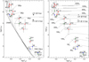 |
Fig. B.1. HRD of stars identified as OB stars in our spectroscopic survey. The coloured sources are the locations with the extinction correction of Indebetouw et al. (2005). The colour coding of the sources indicates in which region they are located: red: field II, green field III and blue field IV, the location of LS1 (Okumura et al. 2000) for the assumed distances of 3.4 and 6 kpc is marked with a “plus” sign (field I). The red squares in panel d are the massive stars classified by Figuerêdo et al. (2008) and Barbosa et al. (2008). Left panel: solid line represents the ZAMS isochrone from Lejeune & Schaerer (2001) and the dashed lines the main-sequence isochrones for 1, 2, 3 and 5 Myr from Ekström et al. (2012) and Yusof et al. (2013). The dash-dot lines represent the PMS isochrones of 1 and 2 Myr from Tognelli et al. (2011). Right panel: dashed lines represent the evolutionary tracks from Ekström et al. (2012) and Yusof et al. (2013). |
Appendix C: Late type stars towards W51
Spectroscopically classified late type stars towards W51.
All Tables
All Figures
|
Fig. 1. Three-colour JHKs-band image from 2MASS of W51 (20′ × 40′), overlaid by 1.1 mm dust continuum contour from the Bolocam survey (Aguirre et al. 2011) in green and the 1.4 GHz NRAO VLA Sky Survey (NVSS, Condon et al. 1998) contours in white. The four white boxes mark the areas where photometry and spectroscopy are obtained. From left to right: field I and II cover HII region G49.5–0.4, field III G49.2–0.3 and field IV covers G48.9–0.3. The yellow arcs mark the location and extent of the 3 subregions in W51: W51A, W51B and W51C used throughout the paper. |
| In the text | |
|
Fig. 2. JHKs composite colour image from the SOFI data of the 4 observed fields in W51, zoomed in on the clusters, from left to right field I, field II, field III and field IV. The red, green and blue channels are mapped to the Ks, H and J, respectively. The regions selected for the photometric analysis are indicated with white circles. The spectroscopically classified massive stars in each field are indicated with their ID numbers. In field II, also the positions of the O stars and massive YSO from Figuerêdo et al. (2008) and Barbosa et al. (2008) are shown. |
| In the text | |
|
Fig. 3. J–Ks vs. Ks colour-magnitude diagram of the four observed fields in W51 showing the positions of all the stars in each field (grey points) and the sub-clusters (black points) defined by the circles on Fig. 2. The red triangles indicate the spectroscopically classified massive stars. The red triangle in panel b is the position of LS1 (note the different y-axis in this panel). The red squares in panel d are the massive stars classified by Figuerêdo et al. (2008) and Barbosa et al. (2008). The blue dashed vertical line represents the un-reddened isochrone for main sequence stars with an age of 1 Myr (Ekström et al. 2012; Yusof et al. 2013). The blue solid line is the reddening-free pre-main-sequence isochrone of Tognelli et al. (2011). The red lines represent the same isochrones, but reddened with AKs = 0.45 mag to highlight the foreground extinction. |
| In the text | |
|
Fig. 4. H–Ks vs. J–H colour-colour diagram of the four observed fields in W51 showing the positions of all the stars in each field (grey points) and the sub-clusters (black points) defined by the circles in Fig. 2. The red triangles indicate the spectroscopically classified massive stars. The red triangle in panel b is the position of LS1. The red squares in panel d are the massive stars classified by Figuerêdo et al. (2008) and Barbosa et al. (2008). The blue dashed lines are the unreddened 1 Myr isochrone (around H–Ks = 0) and reddened with AKs = 3.0 mag (around H–Ks = 2.5 mag). The blue solid lines are the unreddened 1 Myr PMS isochrones and the reddened isochrone with AKs = 3.0 mag. The blue dashed-dotted is the reddening line connecting the high-mass end of the two isochrones. The red lines represent the lines at AKs = 0.45 mag. |
| In the text | |
|
Fig. 5. Normalized K-band spectra of OB-type stars as taken with the multi-object mode of LUCI. The star number and their derived spectral type are indicated. Indicated with dashed lines are the diagnostic lines for the spectral classification. The narrow emission lines at 2.166 μm are of nebular origin (see text). Their profiles are truncated for clarity. |
| In the text | |
|
Fig. 6. Normalized K-band spectrum of source #16, identified as YSO based on the CO bandhead emission. The dashed lines indicate the emission lines in the spectra. |
| In the text | |
|
Fig. 7. HRD of stars identified as OB stars in our spectroscopic survey. The coloured sources are the locations with the extinction correction of Nishiyama et al. (2009). The colour coding of the sources indicates in which region they are located: red: field II, green: field III and blue: field IV. The location of LS1 (Okumura et al. 2000) for the assumed distances of 3.4 and 6 kpc is marked with a “plus” sign. The red squares are the massive stars classified by Figuerêdo et al. (2008) and Barbosa et al. (2008). Left panel: solid line represents the ZAMS isochrone from Lejeune & Schaerer (2001) and the dashed lines the main-sequence isochrones for 1, 2, 3 and 5 Myr from Ekström et al. (2012) and Yusof et al. (2013). The dash-dot lines represent the PMS isochrones of 1 and 2 Myr from Tognelli et al. (2011). Right panel: dashed lines represent the evolutionary tracks from Ekström et al. (2012) and Yusof et al. (2013). |
| In the text | |
|
Fig. 8. Three-colour image of W51 (identical to Fig. 1) overlayed with the annotation of the evolutionary state of the different clusters discussed in Sect. 4.4 as well as the location of the two proto clusters identified in Ginsburg et al. (2012) and the evolved massive star LS1. |
| In the text | |
|
Fig. B.1. HRD of stars identified as OB stars in our spectroscopic survey. The coloured sources are the locations with the extinction correction of Indebetouw et al. (2005). The colour coding of the sources indicates in which region they are located: red: field II, green field III and blue field IV, the location of LS1 (Okumura et al. 2000) for the assumed distances of 3.4 and 6 kpc is marked with a “plus” sign (field I). The red squares in panel d are the massive stars classified by Figuerêdo et al. (2008) and Barbosa et al. (2008). Left panel: solid line represents the ZAMS isochrone from Lejeune & Schaerer (2001) and the dashed lines the main-sequence isochrones for 1, 2, 3 and 5 Myr from Ekström et al. (2012) and Yusof et al. (2013). The dash-dot lines represent the PMS isochrones of 1 and 2 Myr from Tognelli et al. (2011). Right panel: dashed lines represent the evolutionary tracks from Ekström et al. (2012) and Yusof et al. (2013). |
| In the text | |
Current usage metrics show cumulative count of Article Views (full-text article views including HTML views, PDF and ePub downloads, according to the available data) and Abstracts Views on Vision4Press platform.
Data correspond to usage on the plateform after 2015. The current usage metrics is available 48-96 hours after online publication and is updated daily on week days.
Initial download of the metrics may take a while.