| Issue |
A&A
Volume 624, April 2019
|
|
|---|---|---|
| Article Number | A107 | |
| Number of page(s) | 13 | |
| Section | Interstellar and circumstellar matter | |
| DOI | https://doi.org/10.1051/0004-6361/201834864 | |
| Published online | 19 April 2019 | |
Interferometric observations of SiO thermal emission in the inner wind of M-type AGB stars IK Tauri and IRC+10011★,★★
1
Molecular Astrophysics Group, Instituto de Física Fundamental (IFF-CSIC),
C/Serrano 123,
28006
Madrid, Spain
e-mail: This email address is being protected from spambots. You need JavaScript enabled to view it.
2
Observatorio Astronómico Nacional (OAN-IGN),
C/Alfonso XII 3,
28014
Madrid, Spain
3
Observatorio Astronómico Nacional (OAN-IGN),
Apdo 112,
28803
Alcalá de Henares,
Madrid, Spain
4
Instituto Geográfico Nacional, Centro de Desarrollos Tecnológicos, Observatorio de Yebes,
Apdo 148,
19080
Yebes, Spain
5
Institut de Radioastronomie Millimétrique,
300 rue de la Piscine,
38406
Saint Martin d’Hères, France
Received:
14
December
2018
Accepted:
25
February
2019
Abstract
Context. Asymptotic giant branch (AGB) stars go through a process of strong mass loss that involves pulsations of the atmosphere, which extends to a region in which the conditions are adequate for dust grains to form. Radiation pressure acts on these grains which, coupled to the gas, drive a massive outflow. The details of this process are not clear, including which molecules are involved in the condensation of dust grains.
Aims. We seek to study the role of the SiO molecule in the process of dust formation and mass loss in M-type AGB stars.
Methods. Using the IRAM NOEMA interferometer we observed the 28SiO and 29SiO J = 3−2, v = 0 emission from the inner circumstellar envelope of the evolved stars IK Tau and IRC+10011. We computed azimuthally averaged emission profiles to compare the observations to models using a molecular excitation and ray-tracing code for SiO thermal emission.
Results. We observe circular symmetry in the emission distribution. We also find that the source diameter varies only marginally with radial velocity, which is not the expected behaviour for envelopes expanding at an almost constant velocity. The adopted density, velocity, and abundance laws, together with the mass-loss rate, which best fit the observations, give us information concerning the chemical behaviour of the SiO molecule and its role in the dust formation process.
Conclusions. The results indicate that there is a strong coupling between the depletion of gas-phase SiO and gas acceleration in the inner envelope. This could be explained by the condensation of SiO into dust grains.
Key words: stars: AGB and post-AGB / stars: mass-loss / stars: late-type / circumstellar matter / radio lines: stars
The reduced datacubes are only available at the CDS via anonymous ftp to cdsarc.u-strasbg.fr (130.79.128.5) or via http://cdsarc.u-strasbg.fr/viz-bin/qcat?J/A+A/624/A107
This work is based on observations carried out under project number W15BJ with the IRAM NOEMA interferometer. IRAM is supported by INSU/CNRS (France), MPG (Germany), and IGN (Spain).
© ESO 2019
1 Introduction
During the asymptotic giant branch (AGB) phase, stars go through a process of strong mass loss that is caused by the pulsating levitation of the atmosphere, transporting gas to a region in which the conditions are right for dust condensation (i.e. low temperature and high density). Dust is then accelerated by radiation pressure from the central star, and as a consequence of the efficient coupling between gas and dust, drives a massive outflow. This outflow becomes part of the interstellar medium after forming a circumstellar envelope and a planetary nebula in future post-AGB phases (Höfner & Olofsson 2018). In a mature galaxy like the Milky Way, stars of low to intermediate mass (those with an initial mass between 0.8 and 8 M⊙) are responsible for a considerable fraction of the reinsertion of material into the galaxy due to such massive molecule-rich winds (Busso et al. 1999).
AGB stars consist of a carbon-oxygen core, a helium-burning shell, and a more external hydrogen-burning shell1. Eventually the helium shell runs out of fuel, but in periods of ~104–105 yr the hydrogen burning shell provides the inner shell with enough helium for an explosive event to take place, where helium burns again. This causes the hydrogen shell to cease burning and results in an expansion of the stellar atmosphere. These periodic events are known as thermal pulses. In this way the star enters the thermally pulsing asymptotic giant branch (TP-AGB), and the related third dredge-up events lifts up carbon and other elements to the outer atmosphere. Depending on the duration of the TP-AGB, which depends on the initial mass, some stars become C-rich ([C] > [O]) and some remain O-rich (i.e. M-type) during the whole evolution. C-rich chemistry is fairly well understood and has been shown to be feasible in stellar outflow conditions (Gail & Sedlmayr 1984). But the same cannot be said about O-rich chemistry, for which the process of nucleation and growth of dust grains is not clear (see e.g. Gobrecht et al. 2016; Gail et al. 2016). According to observations, the dominating dust components formed in the photospheres of M-type stars are magnesium iron silicates (Molster et al. 2010), and laboratory investigations support this assessment (Vollmer et al. 2009; Nguyen et al. 2010; Bose et al. 2010). More recently it has been found that for objects with low mass-loss rates alumina dust may be as abundant as silicate dust (Zhao-Geisler et al. 2012; Karavikova et al. 2013; Khouri et al. 2015).
Among all the gas-phase species of refractory elements that could be involved in the dust nucleation process, SiO is one of the most abundant. Dust containing Si and O are also identified through the 9 and 18 μm silicate features in infrared spectra of stars (Forrest et al. 1975; Pégourié & Papoular 1985). Therefore, the SiO gas-phase abundance should fall off as the molecules are incorporated into dust grains. At the same time, the expansion velocity of the gas should increase as the radiation pressure acts more efficiently on dust grains of larger size. By the determination of the abundance of SiO and its dynamical behaviour throughout the envelope we can assess if a relation between SiO depletion and dust formation exists. Other alternatives to explain dust formation in O-rich stellar atmosphereshave been studied recently by, for example Goumans & Bromley (2012), Plane (2013), and Bromley et al. (2014).
Thermal2 emission from the SiO molecule was previously studied by Bujarrabal et al. (1989) with the Institut de Radioastronomie Millimétrique (IRAM) 30 m radio antenna and has given us information about the physical conditions of the circumstellar envelope. These authors also observed the CO molecule and simultaneously modelled the emission from both CO and SiO. There are also interferometric observations of SiO that suggest that the gas might not reach its final expansion velocity as fast as was previously believed and that dust formation might also not occur as instantaneously (Lucas et al. 1992). These authors found a relatively large initial abundance of gaseous SiO, X(SiO) ~5 × 10⁻⁵, which has a strong decrease beyond ~1015 cm from grain formation, which would itself be associated with the gas acceleration3 (see also Bujarrabal & Alcolea 1991).
González-Delgado et al. (2003) carried out a statistical analysis on a sample of AGB stars. They found a relation between the radius of the SiO envelope and what they called the “density measure”, Ṁ∕Ve, where Ṁ is the stellar mass-loss rate and Ve is the expansion velocity. They deduced, in most objects, relatively lower inner abundances: X(SiO) ≤ 10−5, and stressed the importance of photodissociation in establishing the outer SiO-rich boundary. On the other hand Schöier et al. (2004) concluded that X(SiO) is as high as 4 × 10⁻⁵ in the inner envelope and has a decrease that is higher than a factor 10, due to grain formation, at ~ 1015 cm. According to these authors, a small fraction of SiO remained in the gas until photodissociation. Decin et al. (2010) also modelled several emission lines from observations carried out with various radio telescopes and obtained their own set of physical parameters for the envelope. Later on Decin et al. (2018) carried out a spectral line and imaging survey to observe molecular species key to the formation of dust grains, providing constraints on the properties of oxygen-dominated stellar winds. These authors concluded that properties tend to be different for stars with high mass-loss rates as compared to those with low mass-loss rates and found a similar stratification of the SiO abundance starting with a somewhat lower value.
We conducted observations of two evolved, O-rich, stars with intermediate mass-loss rates, IK Tau and IRC+10011 (a.k.a. WX Psc), with the NOrthern Extended Millimeter Array (NOEMA) interferometer, resulting in higher spatial resolution than previously available. We describe the observations and data reduction in Sect. 2 and discuss the results in Sect. 3. We obtained the best fit for the azimuthally averaged emission using a molecular excitation and line transfer code. The resulting models and physical parameters obtained are shown and discussed in Sect. 4, where we also discuss the implications for dust formation. Final discussion and conclusions are shown in Sects. 5 and 6.
2 Observations
Observations were carried out towards IK Tau and IRC+10011 with the NOEMA millimeter interferometer (project W15BJ) during the winter and autumn of 2016 using seven and eight antennas. The observations were performed by alternating between the two sources in cycles of ~15 min in the so-called track-sharing mode. Acquisitions were obtained from February 21 to 24, 2016 for the most extended A configuration, and between October 10 and 31, 2016 for the C configuration. In the merged data we obtained baselines ranging from 48 to 720 m, for a total of about 5 h on each source. Data were recorded with the Widex Correlator for 4 GHz bandwidth with two polarisations and a channel spacing of 2 MHz. In addition, observations of one receiver polarisation were simultaneously processed by the narrow-band correlator to achieve a spectral resolution of 0.3 MHz in a windowof 110 MHz around the frequencies 130.269 and 128.637 GHz, which are the rest frequencies of the J = 3−2, v = 0 emission lines for 28SiO and 29SiO, respectively;these comprise our two lines of interest.
The data calibration was performed with CLIC, which is part of the GILDAS4 package. Two phase calibrators were observed, each one close to one of the sources, also in cycles of 15 min. The bright quasars 3C84 and 3C454.3 (with more than 15 Jy in continuum emission) were observed for the bandpass calibration, and acquisitions in MWC349 and LKHA101 (the standard flux calibrators for the NOEMA observatory) were used to reach an absolute flux accuracy in the calibrated data better than 10%. The achieved relative flux accuracy among our observed objects and transitions is nonetheless better than 10%.
Maps ina central channel for both objects and both isotopologues are shown in Figs. 1 and 2. The continuum emission was subtracted to better identify the weak emission at extreme velocities. A synthetic half-power beam size of 1′′ × 1′′ in diameter was obtained with data robust weighting. The detailed data inspection was performed in 120 channels with spectral resolutions of 0.6 km s−1. Data reduction was carried out with standard reduction techniques using MAPPING (also included in the GILDAS package). The reported systemic velocities of the sources are 34.4 and 9.6 km s−1 for IK Tau and IRC+10011, respectively (González-Delgado et al. 2003).
3 Results: size and flux
In Figs. 3 and 4 we show the half-power angular diameters and fluxes as functions of local standard of rest (LSR) velocity determined from model fits to the visibilities obtained for IK Tau and IRC+10011. The model used to represent the emission region was that of a Gaussian disc. We note that the size of the SiO emission region is extended for both objects, with angular diameters of ~2.′′5 for IK Tau and ~2 for IRC+10011, which translate to physical diameters of the order of 1 × 1016 cm and 2 × 1016 cm, respectively, when considering the distances to the objects shown in Table 1.
The plots for both 28SiO and 29SiO show that the diameter does not decrease with offset from the central velocity; instead, the diameter is very similar in the line centres and wings. Lucas et al. (1992) argued that this can be explained if the final expansion velocity has not been fully reached in the inner SiO emission region. In such a case the hot, central regions emit only at the central velocities, while only the outer regions are seen at the profile edges with a larger apparent size than if the velocity were constant. On the contrary, Sahai & Bieging (1993) found no need for such slowly varying velocity fields. Instead, they argued that this behaviour is a characteristic feature of power-law intensity distributions, being scale-free, rather than Gaussian, where there are well-defined scale sizes. Nonetheless, attempting other types of fits, such as uniform disc, exponential and power-law, resulted in considerably larger errors in the fits to the observational data; therefore we believe that a Gaussian disc accurately represents the emission region and that indeed gas is still accelerating in the inner envelope.
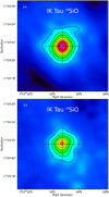 |
Fig. 1 SiO emission maps in one of the central channels for IK Tau in 28SiO (top) and 29SiO (bottom). Contour level spacings are 200 mJy beam−1 for 28SiO and 50 mJy beam−1 for 29SiO. In the top left corner the channel LSR velocity is indicated. |
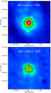 |
Fig. 2 SiO emission maps in one of the central channels for IRC+10011 in 28SiO (top) and 29SiO (bottom). Contour level spacings are 100 mJy beam−1 for 28SiO and 20 mJy beam−1 for 29SiO. In the top left corner the channel LSR velocity is indicated. |
4 Radiative transfer and SiO abundance
To estimate the physical parameters that reproduce the emission we used a radiative transfer code assuming spherical symmetry. The parameters are fed into a molecular excitation and ray-tracing code that solves the statistical equilibrium equations by assuming the Sobolev approximation, i.e. describing photon trapping by means of an escape-probability algorithm. Level populations were then used to calculate the expected intensity for a high number of rays in the direction of the line of sight, following the standard radiative transfer equation. We take into account 40 rotational levels in the v = 0 vibrational state. The black-body stellar radiation field with stellar temperatures listed in Table 2 is taken into account for radiative excitation. The dust radiation field is not taken into account. Finally, the brightness distributions are convolved with the telescope beam to simulate the observational maps. Similar codes were used by Bujarrabal et al. (1989) and Bujarrabal & Alcolea (1991), where more details on the numerical treatment can be found. Collisional transition probabilities were taken from the Leiden Atomic and Molecular Database (LAMDA5; Schöier et al. 2005). We find that the level populations are practically thermalised for 28SiO, but not for 29SiO owing to its lower opacities.
From the observations we calculated azimuthal averages of the emission and then computed an extensive number of models for the physical parameters of the circumstellar envelope to reproduce the azimuthally averaged emission maps. The computation of the azimuthal averages allows us to gain signal-to-noise ratio (S/N) in the outer parts of the map and to compare lines at all distances with our molecular excitation and radiative transfer code. The code was tailored to efficiently treat optically thin and optically thick thermal SiO emission. The observations, together with the best-fitting model results, are shown in Figs. 5 and 6.
The criteria used to determine the goodnes of fit to a model are as follows:
to fit both isotopic species with the same parameters varying only their relative abundance, assuming that photodissociation is not isotope selective;
to obtain a reasonable and similar value for the 28SiO/29SiO ratio for both objects;
to take previously published kinetic temperature and expansion velocity laws as starting points;
to fix mass-loss rates, terminal velocities, and distances to agree with previously published values.
We considered that the density is a function of the radius, mass-loss rate, and expansion velocity following the continuity equation
 (1)
(1)
where Ṁ is the mass-loss rate, Ve is the expansion velocity, and r is the distance from the central star.
The kinetic temperature profiles were determined using the following equation:
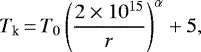 (2)
(2)
where T0 and α are free parameters that determine the magnitude and slope of the kinetic temperature.
The velocity profile has been parameterised using a simplified law (Lamers & Cassinelli 1999). We used the following expression:

where V0 is the velocity before the gas starts to accelerate, which is set to 1 km s−1, V∞ is the terminal expansion velocity, and Rd is the distance from the star at which dust grains form, which we treated as a free parameter that affects the innermost portion of the envelope, where little is known about the dynamics.
To describe the SiO relative abundance profile we used a simplified parameterisation
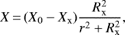 (5)
(5)
where Xx is the final abundance left after SiO depletion in the inner envelope, and X0 is treated as a free parameter that represents a reference abundance such that the initial value for X is X0 − Xx. We assumed that 85% of the gas-phase SiO is condensed into dust grains for both objects, following Bujarrabal et al. (1989). The SiO abundance distribution is nonetheless expected to be very complicated because of its strong dependence on dust parameters, in particular the dust mass loss rate (González-Delgado et al. 2003). As can be seen, Rx is the distance from the central star at which the abundance falls to  (X0 − Xx).
The values of the fixed parameters adopted for each object are given in Table 1. The value for the distance to IK Tau is taken from the Gaia Data Release 2 (Gaia Collaboration 2018), while that of IRC+10011 is taken from Vinkovic et al. (2004) and references therein. We adopt the mass-loss rates reported in Lucas et al. (1992) for both objects, which have been corroborated by other more recent works (see e.g. Decin et al. 2018). Stellar temperatures used to calculate stellar excitation are taken from Decin et al. (2018) for IK Tau and Vinkovic et al. (2004) for IRC+10011. Terminal expansion velocities were taken from Velilla-Prieto et al. (2017) and Vinkovic et al. (2004) for IK Tau and IRC+10011, respectively. We fixed 28SiO/29SiO = 20 for both objects, similar to the galactic value and in agreement with the values obtained by Monson et al. (2017).
The free parameters and their values are listed in Table 2. The density, kinetic temperature, abundance, and expansion velocity for the models of both sources are shown in Figs. 7 and 8. For both objects we found kinetic temperature laws somewhat in between those of Bujarrabal et al. (1989) and Decin et al. (2010). Our results are plotted in Figs. 7 and 8. We note that these laws were obtained for IK Tau, but we also included them in the plots for IRC+10011 for comparison. The kinetic temperature found by Bujarrabal et al. (1989) is higher in general, but decreases steeply as r−0.9, while that of Decin et al. (2010) decreases more slowly as r−0.6.
While having observations of two isotopologues for two relatively similar sources helps us to more strictly constrain the parameters in our models, it also results in complications in the achievement of satisfactory model fits and in the calculation of uncertainties. The criteria to obtain the parameters of the model that best fit the observations were the following: from the azimuthally averaged emission maps that resulted from the observations we calculated the rms value of the noise. It is calculated outside the emission region in emitting LSR velocities to account for cleaning errors and we call it σ.
We computed a set of models representing different scenarios, such as slow/fast acceleration, early/late SiO depletion, and we obtained maps of azimuthally averaged emission. We visually inspected the model maps and compared these maps with the azimuthally averaged emission maps that resulted from the observations to infer which models reproduced the observations better, and to identify problems and artefacts that would be hard to identify numerically. Additionally, we subtracted the observed map from each resulting model map, thereby obtaining a residual map. In this residual map we calculated the rms in the zones with emission, and also inspected the maps visually to identify zones of large residual value and/or other systematic errors. The model we chose as the most adequate is the one that results in the residual map with the minimum rms and minimum residual value. This process is done simultaneously for both 28SiO and 29SiO emission because the set of parameters has to reproduce the emission for both isotopic species varying only their relative abundance to H2. Some compromise had to be made because while the variation of a given parameter might improve the fit for an isotopic species, at the same time it could worsen the fit for the other.
Once we had the general idea of the scenario, we then computed another set of models with slighter variations of the parameters and chose the most adequate model in the same manner that we did in the previous step and also for both isotopologues simultaneously. We established as the most adequate models those that satisfy the following conditions for both isotopic species: the rms in the emission region stays below 3σ, the maximum residual has an absolute value below 5σ, and the size of the region with this maximum residual stays smaller than the beam size.
Once we had established the set of parameters that best reproduced the observations, to estimate the uncertainties in these parameters (see Table 2) we varied one parameter at a time while keeping the others constant and obtained residual maps. Once the map contained residuals with values exceeding 7 σ or had a rms in the region with emission exceeding 3σ for either of the isotopic species, we regarded that model as no longer acceptable and reported the uncertainties as the maximum variation the parameter can take; we also always visually inspected the maps. A more detailed description of the method is given in Appendix A.
Another source of uncertainty is the fact that we constrained the kinetic temperature law by a single SiO line, however our results for IK Tau agree with those of Bujarrabal et al. (1989; see Fig. 7). These authors used CO (J = 1−0) and SiO (J = 2−1) lines to constrain the kinetic temperature profile. Unfortunately, to our knowledge, similar information for IRC+10011 is not available.
As we can see in Figs. 7 and 8, the best fits are those which result from a gas that is still accelerating in the inner region of the wind and that has not acquired its terminal expansion velocity as quickly as itwas previously believed (see e.g. Olofsson et al. 1982; Morris et al. 1983; Schönberg 1988). We find that there is a good correlation between the decrease in the abundance of the SiO molecule and the gas acceleration. If the SiO is removed from the gas phase as a result of grain growth, radiation pressure from the star then acts more efficiently on larger dust grains. Owing to a strong coupling between gas and dust, gas then accelerates along with the dust. Therefore, a correlation between gas-phase SiO depletion and gas acceleration might be a sign of SiO condensation into dust grains. Our results indicate that it is reasonable to assume that ~85% percent of the SiO molecular gas condenses into dust grains, and the remaining SiO photodissociates very far from the star. We also note that gas acceleration and SiO depletion happen slightly faster for IRC+10011 than for IK Tau. This is understandable if we take into account the larger mass-loss rate, and hence larger density, of the former: under this condition grain growth happens more quickly, and therefore the dust accelerates faster and SiO depletion also happens faster. For this object we also assumed that the value of the temperature is in general lower, which also favours the condensation of dust grains.
After the molecular gas is condensed into dust, at much larger distances from the star, photodissociation removes the remaining SiO in the gas phase. We assumed that photodissociation sets in at a distance beyond 3 × 1016 cm for both objects following the results of Li et al. (2016). Using a large gas-phase chemical model of an AGB envelope including the effects of CO and N2 self-shielding, along with an improved list of parent species derived from detailed modelling and observations, concluded that the SiO photodissociation region lies past 3 × 1016 cm for IK Tau.
In Fig. 9 we show azimuthally averaged spectra obtained from observations of 29SiO in IK Tau and spectra that results from the modelling. We can see two interesting features of the obervations that were reproduced in the models to some extent. One is is self-absorption and the other is a triple-peaked structure of the azimuthally averaged central spectra. Self-absorption happens when a region of relatively low excitation temperature lies somewhere along the line of sight to a hotter region with the same radial velocity. The other feature, the triple-peaked central spectra, means that we find local maxima at central velocities, as well as in the blue and red regions of the spectra. The blue and red peaks are very common in optically thin emission of outflows because we see the approaching and receding wind. The central peak appears if we have a high SiO abundance in the inner zone with slow-moving gas causing an emission excess. The three peaks can clearly be seen as well as the self-absorption in the blue-shifted side of the spectra. The figures include the emission at six offsets from the central star separated by 0.′′125 to make the effects more visible.
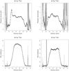 |
Fig. 3 Half-power diameter and flux as functions of LSR velocity as determined from model fits to the visibilities for IK Tau. As argued in Lucas et al. (1992), the small variation of the diameter as a function of velocity could be explained by a wind for which the final expansion velocity is not yet fully reached. |
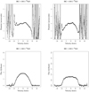 |
Fig. 4 Half-power diameter and flux as functions of LSR velocity as determined from model fits to the visibilities for IRC+10011.The small variation in the diameter as a function of velocity could be explained by a wind for which the final expansion velocity is not yet fully reached. |
Fixed parameters used for the models.
Free parameters used for the models.
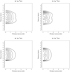 |
Fig. 5 Azimuthally averaged emission as a function of distance and LSR velocity for IK Tau. Observations are represented on the top and results of the radiative transfer model on the bottom. Both isotopologues are shown: 28SiO on the left and 29SiO on the right. Countour labels are denoted in units of Jy beam−1. |
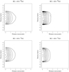 |
Fig. 6 Azimuthally averaged emission as a function of distance and LSR velocity for IRC+10011. Observations are represented on the top and results of the radiative transfer model on the bottom. Both isotopologues are shown: 28SiO on the left and 29SiO on the right. Countour labels are denoted in units of Jy beam−1. |
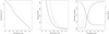 |
Fig. 7 Total density, kinetic temperature, molecular abundance, and velocity profile used for the models of Fig. 5 for IK Tau. We also show for comparison the temperatures obtained by Bujarrabal et al. (1989; dashed line) and Decin et al. (2010; dotted line). In the velocity plot we include, for comparison, the velocity by Decin et al. (2010; dotted line). The velocity stays constant at 1 km s−1 up to the distance Rd, and then gradually increases as described in Eqs. (3) and (4). |
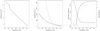 |
Fig. 8 Total density, kinetic temperature, molecular abundance, and velocity profile used for the models of Fig. 6 for IRC+10011. We also show for comparison the temperatures obtained by Bujarrabal et al. (1989; dashed line) and Decin et al. (2010; dotted line) for IK Tau. In the velocity plot we include, for comparison, the velocity by Decin et al. (2010) for IK Tau (dotted line). The velocity stays constant at 1 km s−1 up to the distance Rd, and then gradually increases as described in Eqs. (3) and (4). |
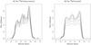 |
Fig. 9 Spectra of the innermost regions of the envelope. The azimuthally averaged observed emission is shown to the left and the model to the right. Six positions are shown separated by 0.′′125; the innermost is the most intense. The model reproduces to some extent the three peaks and the self-absorption that happens in the blue-shifted side of the spectra. |
5 Discussion
We have been able to reproduce, quantitatively and qualitatively, the emission from the inner envelope of IK Tau and IRC+10011 within the expected uncertainties, including the effects of self-absorption, as can be seen especially in the blue part of the spectrum of the 29SiO emission. We also reproduce in the models the triple-peaked structure of the azimuthally averaged central spectra. The central peak appears because we have a high SiO abundance in the inner zone with slow-moving gas that causes an emission excess. This supports our hypothesis that the inner part of the envelope is richer in gas-phase SiO and is moving at lower velocities before the gas accelerates and strong SiO depletion occurs.
The sizes of the SiO emission we computed (Sect. 3) differ to those found by González-Delgado et al. (2003). For IK Tau these authors found a radius of the SiO emission region of 2.5 × 1016 cm, which is larger than the value we found by a factor of 4.6. It is worth noting that in their work the radius was set as a free parameter, and they reported the radius value that provided the best fit. We also note that they used the rather high mass-loss rate of 3 × 10⁻⁵ M⊙ yr−1 compared to the value of 5 × 10⁻⁶ M⊙ yr−1 used by us. Our values are, nonetheless, very similar to those found by Lucas et al. (1992), taking into account that they underestimated the distances to the sources.
The value of the terminal expansion velocity for IK Tau agrees with that found by Velilla-Prieto et al. (2017), who estimated an expansion velocity of 18.5 km s−1 from the line widths of the spectral features arising from the outer envelope, where the gas is assumed to have fully accelerated to its maximal velocity. The value for this terminal expansion velocity is higher than the previously found value of 17 km s−1 (Lucas et al. 1992).
6 Summary and conclusions
Using high angular resolution images of SiO thermal emission in the circumstellar envelopes of IK Tau and IRC+10011 we estimated the half-power diameters and fluxes as functions of velocity assuming the emission region is well represented by a Gaussian disc. We conclude that the fact that the variation of the diameter of the emission region is small is a sign that gas is still accelerating in the inner envelope where dust grains are forming. Assuming spherical symmetry we computed azimuthal averages. We were able to estimate the physical parameters that reproduce the emission using a molecular excitation and ray-tracing code tailored to treat SiO thermal emission. We used as starting points for our models previously found values of parameters such as mass-loss rate, distance, stellar temperature, and terminal velocity. We used temperature laws, expansion velocity laws, and isotopic ratios, which are in agreement with values previously reported in the literature. We conclude there is a strong coupling between the depletion of gas-phase SiO and gas acceleration in the inner region of the envelope. Both the SiO depletion and gas acceleration could be explained by the condensation of SiO into dust grains. The difference inacceleration and SiO depletion between the two objects can be explained in terms of their mass-loss rates and temperatures. SiO depletion and gas acceleration occur faster in the higher mass loss, lower temperature object because the appropriate conditions for dust formation appear sooner and at shorter distances from the star.
Acknowledgements
The research leading to these results has received funding from the European Research Council under the European Union’s Seventh Framework Programme (FP/2007-2013) / ERC Grant Agreement n. 610256 NANOCOSMOS and by the Spanish MINECO, Grant FIS2012-32096. This work has made use of data from the European Space Agency (ESA) mission Gaia (https://www.cosmos.esa.int/gaia), processed by the Gaia Data Processing and Analysis Consortium (DPAC, https://www.cosmos.esa.int/web/gaia/dpac/consortium). Funding for the DPAC has been provided by national institutions, in particular the institutions participating in the Gaia Multilateral Agreement. The authors thank the anonymous referee for comments and suggestions that improved the quality of the manuscript. This research has made use of NASA’s Astrophysics Data System.
Appendix A Obtaining the best-fit model and parameter uncertainties
We illustrate the method used to obtain the models that best fit the observations. In Fig. A.1 we show the azimuthally averaged emission map obtained from the observations. The rectangle outside the contours represents the area where the observational rms value of the noise is calculated. We chose this region to take into account errors resulting from the cleaning process. We call this rms value, σ. For this particular case we have σ ~ 0.07 Jy beam−1.
We compute a set of models varying the parameters for the abundance, expansion velocity, and kinetic temperature laws to account for different scenarios, i.e. slow or fast acceleration, SiO depletion happening sooner or later, etc. We compute azimuthally averaged maps of the emission from the models. Besides visually inspecting and comparing each of the resulting models to the observations, we subtract from the model map the observed map and obtain a residual map. Our goal is to obtain a model that results in a residual map with the minimum rms in the emission zone. We cannot rely solely on this criterion to discriminate between models, as it can average out large residuals with the very small. Therefore, we use as an additional criterion that the zones with maximum residuals must have an absolute value below 5σ and a size no more extended than the size of the beam.
Once we find the general trends for the abundance, expansion velocity, and kinetic temperature laws that best reproduce the observations, we start from there and vary each of the parameters slightly until we find the model that results in the residual map with the minimum rms and the minimum residual values.
If we subtract the observations from the model, for the case of 28SiO emission shown in Fig. 5, we obtain the residual map shown in Fig. A.2. When we calculate the value of the rms of this map in the region with emission, represented by the rectangle, we obtain a value of ~0.09 Jy beam−1, which is ~1.3 σ. This is done while also visually inspecting the resulting models to avoid other systematic errors. For this particular case, the absolute value of the largest residual is ~0.28 Jy beam−1 (4σ) and is located in the regions enclosed by the red contours.
The fact that the same set of parameters has to satisfy the observations for both isotopologues, as we assumed that photodissociation is not isotope selective, complicates the process, since variations of the parameters that improve the fit for one of the isotopic species, might at the same time worsen it for the other. For this reason the modelling process was carried out for both isotopologues simultaneously and some compromise had to be made. The model we chose as the best-fit results in a residual map with an rms below 3σ and contains no residual values greater than 5σ. Additionally, the zones with high residuals cannot exceed the size of the beam. Visual inspection was performed on all maps to confirm.
For the same object, but for observations of 29SiO (See Fig. A.3), we calculate σ in the region enclosed by a rectangle to the right of the contours. We obtain σ ~ 0.02 Jy beam−1, smaller thanthat obtained for 28SiO. When we subtract the model map shown in Fig. 5 from the observations map, we obtain the residual map shown in Fig. A.4. In this case the rms in the emission region is ~0.04 Jy beam−1 (2σ) and the largest value of the residual is ~0.1 Jy beam−1 (5σ). Further changing the parameters either increases the rms value of the residual map, or the largest value of the residual for one of the isotopologues, therefore we conclude that this is the model that best fit the observations for both isotopic species.
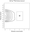 |
Fig. A.1 Azimuthally averaged 28SiO emission as a function of distance and LSR velocity for IK Tau. The rectangle outside the contours represents the area where the rms (σ) was calculated. We chose this region to take into account errors that could have resulted from the cleaning process. |
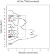 |
Fig. A.2 Residual map that results from subtracting the observations from the model, for IK Tau, 28SiO emission. The rms of the residuals is calculated in the area enclosed by the rectangle. The red contours illustrate the regions in which the maximum, in absolute value, residual is located. |
The uncertainties for the parameters reported in Table 2 were obtained starting from the previously established models. We varied slightly one parameter at the time while keeping the others constant. Besides visually inspecting the resulting model and residualmaps, we calculated the rms and the maximum value of the residual map. Once the rms in the emission region exceeds 3σ or the maximum value of the residual exceeded 7σ, we considered that the model is no longer satisfactory and report the upper and lower uncertainties.
In the case of IRC+10011, 28SiO, the value of the rms of the observations, calculated in the rectangular region indicated in Fig. A.5, is ~0.04 Jy beam−1; the rms in the emission region in the residual map (Fig. A.6) is 0.05 Jy beam−1 (1.25 σ). The maximum residual value is ~0.2 Jy beam−1 (5 σ).
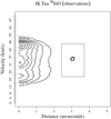 |
Fig. A.3 Azimuthally averaged 28SiO emission as a function of distance and LSR velocity for IK Tau. The rectangle outside the contours represents the area where the rms (σ) was calculated. We chose this region to take into account errors that could have resulted from the cleaning process. |
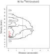 |
Fig. A.4 Residual map that results from subtracting the observations from the model, for IK Tau, 29SiO emission. The rms of the residuals is calculated in the area enclosed by the rectangle. The red contours illustrate the regions where the maximum residual, in absolute value, is located. |
For 29SiO emission in the case of IRC+10011, we obtain a rms value of the observations ~ 0.012 Jy beam−1 (See Fig. A.7). The rms in the emission region in the residual map (Fig. A.8) is ~0.015 Jy beam−1 (1.25 σ). The maximum residual value is ~0.06 Jy beam−1 (5 σ).
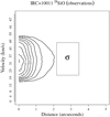 |
Fig. A.5 Azimuthally averaged 28SiO emission as a function of distance and LSR velocity for IRC+10011. The rectangle outside the contours represents the area where the rms (σ) was calculated. We chose this region to take into account errors that could have resulted from the cleaning process. |
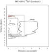 |
Fig. A.6 Residual map that results from subtracting model from observations, for IK Tau, 28SiO emission. The rms of the residuals is calculated in the area enclosed by the rectangle. The red contours illustrate the regions where the maximum residual, in absolute value, is located. |
Given the simplicity of the models, the complexity of the objects, and the infinite number of possible parameterisations, in particular of the SiO abundance, we cannot claim that the resulting models provide a unique fit to the observations. We can only say that they describe a plausible scenario for the conditions in the inner envelope of M-type AGB stars.
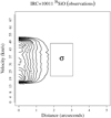 |
Fig. A.7 Azimuthally averaged 28SiO emission as a function of distance and LSR velocity for IRC+10011. The rectangle outside the contours represents the area where the rms (σ) was calculated. We chose this region to take into account errors that could have resulted from the cleaning process. |
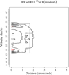 |
Fig. A.8 Residual map that results from subtracting the observations from the model, for IRC+10011, 28SiO emission. The rms of the residuals is calculated in the area enclosed by the rectangle. The red contours illustrate the regions in which the maximum residual, in absolute value, is located. |
References
- Bose, M., Floss, C., & Stadermann., F. J. 2010, ApJ, 714, 1624 [NASA ADS] [CrossRef] [Google Scholar]
- Bromley, S. T., Goumans, T. P. M., Herbst, E., Jones, A. P., & Slater, B. 2014, Phys. Chem. Chem. Phys., 16, 18623 [CrossRef] [Google Scholar]
- Bujarrabal, V., & Alcolea, J. 1991, A&A, 251, 536 [NASA ADS] [Google Scholar]
- Bujarrabal, V., Gómez-González, J., & Planesas, P. 1989, A&A, 219, 256 [NASA ADS] [Google Scholar]
- Busso, M., Gallino, R., & Wasserburg, G. J. 1999, ARA&A, 37, 239 [NASA ADS] [CrossRef] [Google Scholar]
- Decin, L., De Beck, E., Brünken, S., et al. 2010, A&A, 411, 123 [Google Scholar]
- Decin, L., Richards, A. M. S., Danilovich, T., Homan, W., & Nuth, J. A. 2018, A&A, 615, A28 [NASA ADS] [CrossRef] [EDP Sciences] [Google Scholar]
- Duari, D., Cherchneff, I., & Willacy, K. 1999, A&A, 341, L47 [NASA ADS] [Google Scholar]
- Forrest, W. J., Gillet, F. C., & Stein, W. A. 1975, ApJ, 195, 423 [NASA ADS] [CrossRef] [Google Scholar]
- Gaia Collaboration (Brown, A. G. A., et al.) 2018, A&A, 616, A1 [NASA ADS] [CrossRef] [EDP Sciences] [Google Scholar]
- Gail, H. P., & Sedlmayr, E. 1984, A&A, 132, 163 [NASA ADS] [Google Scholar]
- Gail, H. P., Scholz, M., & Pucci, A. 2016, A&A, 591, A17 [NASA ADS] [CrossRef] [EDP Sciences] [Google Scholar]
- Gobrecht, D., Cherchneff, I., Sarangi, A., Plane, J. M. C., & Bromley, S. T. 2016, A&A, 585, A6 [NASA ADS] [CrossRef] [EDP Sciences] [Google Scholar]
- González-Delgado, D., Olofsson, H., Kerschbaum, F., et al. 2003, A&A, 411, 123 [NASA ADS] [CrossRef] [EDP Sciences] [Google Scholar]
- Goumans, T. P. M., & Bromley, S. T. 2012, MNRAS, 420, 3344 [NASA ADS] [Google Scholar]
- Höfner, S., & Olofsson, H. 2018, A&ARv, 26, 1 [NASA ADS] [CrossRef] [Google Scholar]
- Homan, W., Danilovich, T., Decin, L., et al. 2018, A&A, 614, A113 [NASA ADS] [CrossRef] [EDP Sciences] [Google Scholar]
- Karavikova, I., Wittkowsky, M., Ohnaka, K., et al. 2013, A&A, 560, A75 [NASA ADS] [CrossRef] [EDP Sciences] [Google Scholar]
- Kervella, P., Montargès, M., Lagadec, E., et al. 2015, A&A, 578, A77 [NASA ADS] [CrossRef] [EDP Sciences] [Google Scholar]
- Khouri, T., Waters, L. B. F. M., de Koter, A., et al. 2015, A&A, 577, A114 [NASA ADS] [CrossRef] [EDP Sciences] [Google Scholar]
- Lamers, H. J. G. L., & Cassinelli, J. P. 1999, Introduction to Stellar Winds (Cambridge: Cambridge University Press) [CrossRef] [Google Scholar]
- Li, X., Millar, T. J., Heays, A. N., et al. 2016, A&A, 588, A4 [NASA ADS] [CrossRef] [EDP Sciences] [Google Scholar]
- Lucas, R., Bujarrabal, V., Guilloteau, S., et al. 1992, A&A, 262, 491 [NASA ADS] [Google Scholar]
- Molster, F. J., Waters, L. B. F. M., & Kemper, F. 2010, in Lect. Notes Phys., ed. T. Henning (Berlin: Springer Verlag), 815, 143 [Google Scholar]
- Monson, N. N., Morris, M. R., & Young, E. D. 2017, ApJ, 839, 123 [NASA ADS] [CrossRef] [Google Scholar]
- Morris, M., Lucas, R., & Omont, A. 1983, A&A, 142, 107 [Google Scholar]
- Nguyen, A. N., Nittler, L. R., Stadermann, F. J., Stroud, R. M., & Alexander, M. O. 2010, ApJ, 719, 166 [NASA ADS] [CrossRef] [Google Scholar]
- Olofsson, H., Johansson, L. E. B., Hjalmarson, A., & Nguyen-Q-Rieu, M. 1982, A&A, 107, 128 [NASA ADS] [Google Scholar]
- Pégourié, B., & Papoular, R. 1985, A&A, 142, 451 [NASA ADS] [Google Scholar]
- Plane, J. M. C. 2013, Roy. Soc. London Philos. Trans. Ser. A, 371, 20335 [Google Scholar]
- Sahai, R., & Bieging, J. H. 1993, AJ, 105, 595 [NASA ADS] [CrossRef] [Google Scholar]
- Schönberg, K. 1988, A&A, 195, 198 [NASA ADS] [Google Scholar]
- Schöier, F. L., Olofsson, H., Wong, T., Lindqvist, M., & Kerschbaum, F. 2004, A&A, 422, 651 [NASA ADS] [CrossRef] [EDP Sciences] [Google Scholar]
- Schöier, F. L., van der Tak, F. F. S., van Dishoek, E. F., & Black, J. H. 2005, A&A, 432, 369 [NASA ADS] [CrossRef] [EDP Sciences] [Google Scholar]
- Schöier, F. L., David, F., Olofsson, H., Zhang, Q., & Patel, N. 2006, ApJ, 649, 2, 965 [NASA ADS] [CrossRef] [Google Scholar]
- Velilla-Prieto, L., Sánchez-Conteras, C., Cernicharo, J., et al. 2017, A&A, 597, A25 [NASA ADS] [CrossRef] [EDP Sciences] [Google Scholar]
- Vinković, D., Blöcker, T., Hofmann, K.-H., Elitzur, M., & Weigelt, G. 2004, MNRAS, 352, 3, 852 [NASA ADS] [CrossRef] [Google Scholar]
- Vollmer, C., Brenker, F. E., Hoppe, P., & Stroud, R. M. 2009, ApJ, 700, 774 [NASA ADS] [CrossRef] [Google Scholar]
- Zhao-Geisler, R., Quirrenbach, A., Köhler, R., & Lopez, B. 2012, A&A, 545, A56 [NASA ADS] [CrossRef] [EDP Sciences] [Google Scholar]
At the high mass end of AGB stars the core may consist of oxygen and neon, the super AGB stars.
We use the term “thermal” to differenciate between v = 0 emission and maser emission from vibrationally excited states (v > 0), even though SiO excitation is normally far from thermal equilibrium with the gas kinetic temperature so that radiative excitation plays a non-negligible role.
We refer to the relative abundance of SiO with respect to H2 as X(SiO).
All Tables
All Figures
|
Fig. 1 SiO emission maps in one of the central channels for IK Tau in 28SiO (top) and 29SiO (bottom). Contour level spacings are 200 mJy beam−1 for 28SiO and 50 mJy beam−1 for 29SiO. In the top left corner the channel LSR velocity is indicated. |
| In the text | |
|
Fig. 2 SiO emission maps in one of the central channels for IRC+10011 in 28SiO (top) and 29SiO (bottom). Contour level spacings are 100 mJy beam−1 for 28SiO and 20 mJy beam−1 for 29SiO. In the top left corner the channel LSR velocity is indicated. |
| In the text | |
|
Fig. 3 Half-power diameter and flux as functions of LSR velocity as determined from model fits to the visibilities for IK Tau. As argued in Lucas et al. (1992), the small variation of the diameter as a function of velocity could be explained by a wind for which the final expansion velocity is not yet fully reached. |
| In the text | |
|
Fig. 4 Half-power diameter and flux as functions of LSR velocity as determined from model fits to the visibilities for IRC+10011.The small variation in the diameter as a function of velocity could be explained by a wind for which the final expansion velocity is not yet fully reached. |
| In the text | |
|
Fig. 5 Azimuthally averaged emission as a function of distance and LSR velocity for IK Tau. Observations are represented on the top and results of the radiative transfer model on the bottom. Both isotopologues are shown: 28SiO on the left and 29SiO on the right. Countour labels are denoted in units of Jy beam−1. |
| In the text | |
|
Fig. 6 Azimuthally averaged emission as a function of distance and LSR velocity for IRC+10011. Observations are represented on the top and results of the radiative transfer model on the bottom. Both isotopologues are shown: 28SiO on the left and 29SiO on the right. Countour labels are denoted in units of Jy beam−1. |
| In the text | |
|
Fig. 7 Total density, kinetic temperature, molecular abundance, and velocity profile used for the models of Fig. 5 for IK Tau. We also show for comparison the temperatures obtained by Bujarrabal et al. (1989; dashed line) and Decin et al. (2010; dotted line). In the velocity plot we include, for comparison, the velocity by Decin et al. (2010; dotted line). The velocity stays constant at 1 km s−1 up to the distance Rd, and then gradually increases as described in Eqs. (3) and (4). |
| In the text | |
|
Fig. 8 Total density, kinetic temperature, molecular abundance, and velocity profile used for the models of Fig. 6 for IRC+10011. We also show for comparison the temperatures obtained by Bujarrabal et al. (1989; dashed line) and Decin et al. (2010; dotted line) for IK Tau. In the velocity plot we include, for comparison, the velocity by Decin et al. (2010) for IK Tau (dotted line). The velocity stays constant at 1 km s−1 up to the distance Rd, and then gradually increases as described in Eqs. (3) and (4). |
| In the text | |
|
Fig. 9 Spectra of the innermost regions of the envelope. The azimuthally averaged observed emission is shown to the left and the model to the right. Six positions are shown separated by 0.′′125; the innermost is the most intense. The model reproduces to some extent the three peaks and the self-absorption that happens in the blue-shifted side of the spectra. |
| In the text | |
|
Fig. A.1 Azimuthally averaged 28SiO emission as a function of distance and LSR velocity for IK Tau. The rectangle outside the contours represents the area where the rms (σ) was calculated. We chose this region to take into account errors that could have resulted from the cleaning process. |
| In the text | |
|
Fig. A.2 Residual map that results from subtracting the observations from the model, for IK Tau, 28SiO emission. The rms of the residuals is calculated in the area enclosed by the rectangle. The red contours illustrate the regions in which the maximum, in absolute value, residual is located. |
| In the text | |
|
Fig. A.3 Azimuthally averaged 28SiO emission as a function of distance and LSR velocity for IK Tau. The rectangle outside the contours represents the area where the rms (σ) was calculated. We chose this region to take into account errors that could have resulted from the cleaning process. |
| In the text | |
|
Fig. A.4 Residual map that results from subtracting the observations from the model, for IK Tau, 29SiO emission. The rms of the residuals is calculated in the area enclosed by the rectangle. The red contours illustrate the regions where the maximum residual, in absolute value, is located. |
| In the text | |
|
Fig. A.5 Azimuthally averaged 28SiO emission as a function of distance and LSR velocity for IRC+10011. The rectangle outside the contours represents the area where the rms (σ) was calculated. We chose this region to take into account errors that could have resulted from the cleaning process. |
| In the text | |
|
Fig. A.6 Residual map that results from subtracting model from observations, for IK Tau, 28SiO emission. The rms of the residuals is calculated in the area enclosed by the rectangle. The red contours illustrate the regions where the maximum residual, in absolute value, is located. |
| In the text | |
|
Fig. A.7 Azimuthally averaged 28SiO emission as a function of distance and LSR velocity for IRC+10011. The rectangle outside the contours represents the area where the rms (σ) was calculated. We chose this region to take into account errors that could have resulted from the cleaning process. |
| In the text | |
|
Fig. A.8 Residual map that results from subtracting the observations from the model, for IRC+10011, 28SiO emission. The rms of the residuals is calculated in the area enclosed by the rectangle. The red contours illustrate the regions in which the maximum residual, in absolute value, is located. |
| In the text | |
Current usage metrics show cumulative count of Article Views (full-text article views including HTML views, PDF and ePub downloads, according to the available data) and Abstracts Views on Vision4Press platform.
Data correspond to usage on the plateform after 2015. The current usage metrics is available 48-96 hours after online publication and is updated daily on week days.
Initial download of the metrics may take a while.