| Issue |
A&A
Volume 624, April 2019
|
|
|---|---|---|
| Article Number | A44 | |
| Number of page(s) | 9 | |
| Section | Stellar atmospheres | |
| DOI | https://doi.org/10.1051/0004-6361/201834741 | |
| Published online | 05 April 2019 | |
Be and O in the ultra metal-poor dwarf 2MASS J18082002-5104378: the Be–O correlation★,★★
1
GEPI, Observatoire de Paris, Université PSL, CNRS, Place Jules Janssen,
92190 Meudon, France
e-mail: monique.spite@obspm.fr
2
European Southern Observatory,
Casilla 19001,
Santiago, Chile
3
Max Planck Institut für Astronomie,
69117 Heidelberg, Germany
Received:
29
November
2018
Accepted:
14
February
2019
Context. Measurable amounts of Be could have been synthesised primordially if the Universe were non-homogeneous or in the presence of late decaying relic particles.
Aims. We investigate the Be abundance in the extremely metal-poor star 2MASS J1808-5104 ([Fe/H] = −3.84) with the aim of constraining inhomogeneities or the presence of late decaying particles.
Methods. High resolution, high signal-to-noise ratio (S/N) UV spectra were acquired at ESO with the Kueyen 8.2 m telescope and the UVES spectrograph. Abundances were derived using several model atmospheres and spectral synthesis code.
Results. We measured log(Be/H) = −14.3 from a spectrum synthesis of the region of the Be line. Using a conservative approach, however we adopted an upper limit two times higher, i.e. log(Be/H) < −14.0. We measured the O abundance from UV–OH lines and find [O/H] = −3.46 after a 3D correction.
Conclusions. Our observation reinforces the existing upper limit on primordial Be. There is no observational indication for a primordial production of 9Be. This places strong constraints on the properties of putative relic particles. This result also supports the hypothesis of a homogeneous Universe, at the time of nucleosynthesis. Surprisingly, our upper limit of the Be abundance is well below the Be measurements in stars of similar [O/H]. This may be evidence that the Be–O relation breaks down in the early Galaxy, perhaps due to the escape of spallation products from the gas clouds in which stars such as 2MASS J1808-5104 have formed.
Key words: stars: abundances / binaries: spectroscopic / stars: Population II / stars: individual: 2MASS J18082002-5104378
Based on observations collected at the European Organisation for Astronomical Research in the Southern Hemisphere under ESO programmes 101.A-0229(A), (PI M.Spite) and 293.D-5036 (PI J. Mélendez). This research has also made use of Keck Observatory Archive (KOA), operated by the W. M. Keck Observatory and the NASA Exoplanet Science Institute (NExScI), under contract with the National Aeronautics and Space Administration (PI A. Boesgaard).
The 3D values of the oxygen abundance are only available at the CDS via anonymous ftp to cdsarc.u-strasbg.fr (130.79.128.5) or via http://cdsarc.u-strasbg.fr/viz-bin/qcat?J/A+A/624/A44
© M. Spite et al. 2019
 Open Access article, published by EDP Sciences, under the terms of the Creative Commons Attribution License (http://creativecommons.org/licenses/by/4.0), which permits unrestricted use, distribution, and reproduction in any medium, provided the original work is properly cited.
1 Introduction
Beryllium has only one stable isotope, 9Be. The lack of stable nuclei with A = 5 implies that it cannot be synthesised by capture of α particles and the lack of stable nuclei with A = 8 implies that it cannot be synthesised by proton nor neutron captures either. The nuclear fusion reactions that can synthesise Be in a plasma involve several rare nuclei, specifically :  ,
,  , and
, and 
In the conditions that characterise stellar interiors (including H and He burning shells) such reactions cannot synthesise Be fast enough to counter the inverse photodissociation reactions that destroy this element. Thus stars are net destroyers of Be.
In the first minutes of existence of the primordial plasma when most of the helium in the Universe was produced, very tiny amounts of 9Be can be formed; this can occur at the level of log(9Be/H) ≈ 10−18 (Pitrou et al. 2018), that is almost eight orders of magnitude less than the primordial 7Li. This is however true under “standard” conditions, that is if the plasma is homogeneous and there is no “new physics”. If the primordial plasma was inhomogeneous and in particular included lower density n-rich regions, Boyd & Kajino (1989) showed that 3H and 7Li could be abundant enough to make the  reaction, which is an efficient channel to produce sizeable amounts of 9Be. A way to introduce new physics is to postulate the existence of relic particles, interacting either electromagnetically or strongly, which decay at late times (see e.g. Jedamzik 2006; Kusakabe et al. 2009, and references therein). For example, Pospelov & Pradler (2011) showed that the energy injected by decaying hadrons can lead to an efficient 9 Be production via the
  reaction. Infact they advocate the use of an upper limit on the primordial 9 Be abundance as a powerful test to put limits on the energy and decay half-life of such putative relic hadrons. The common wisdom, supported by the observations (see below) is that all the observed Be is produced by spallation processes triggered by cosmic rays in the interstellar medium (Reeves et al. 1970; Meneguzzi et al. 1971).
From the observational point of view, Be can be observed in solar-type stars via the Be ii resonance doublet at 313 nm. This makes the observation from the ground difficult since this wavelength is rather near to the atmospheric cut-off. The Be abundance in the Sun was determined using the lines from Chmielewski et al. (1975) who derived a Be abundance about 0.3 dex lower than the meteoritic abundance. Coupled to the fact that soon after, Boesgaard (1976) found almost the same Be abundance in a sample of young stars, this uniformity led to the notion that Be is depleted in the Sun, like Li. The solar abundance of Be was drastically revised by Balachandran & Bell (1998) who invoked the presence of an unaccounted continuum opacity at UV wavelengths and derived a Be abundance that is in good agreement with the meteoritic abundance. The motivation for this extra opacity was to force the UV and IR lines to yield the same O abundance. An analysis of these lines using 3D hydrodynamical simulations by Asplund (2004) confirmed the need for this extra opacity. It should be noted however that the source of this continuum opacity has not to date been identified and that it is not unanimously accepted (see e.g. Boesgaard & King 2002).Recently Carlberg et al. (2018), using a new line list in the near UV for generating theoretical solar spectra in the region of the Be lines, found that the difference in Be abundance is only 0.2 dex with or without an extra opacity. This implies that even using this extra opacity, Be is depleted by about 0.1 dex in the solar photosphere.
The first attempts to measure Be in Pop II stars to study the Galactic evolution of Be, began in the 1980s (Molaro & Beckman 1984; Molaro 1987), however it was not until the late 1980s and 1990s that it became clear that the Be abundance shows a clear linear decrease with decreasing metallicity (Rebolo et al. 1988; Gilmore et al. 1991, 1992; Ryan et al. 1992; Boesgaard & King 1993; Molaro et al. 1997). If Be is produced only by cosmic rays, then the Be abundance can be used as chronometer, provided there is a suitable model of the temporal evolution of the cosmic ray evolution (Beers et al. 2000; Pasquini et al. 2005). The advent of 8 m class telescopes with high resolution spectrographs that can observe down to the atmospheric cut-off allowed the measurement of Be in a large sample of field halo stars (Boesgaard et al. 1999, 2011; Primas et al. 2000a,b; Boesgaard 2007; Smiljanic et al. 2009; Ito et al. 2009; Tan et al. 2009; Tan & Zhao 2011) and also in two globular clusters (Pasquini et al. 2004, 2007).
Be abundances in metal-poor stars allow for probing the existence of inhomogeneities in the primordial Universe or the existence of late decaying relic particles. If there is no primordial production of Be, the linear decrease of the Be abundance with decreasing metallicity should continue no matter how low the metallicity of the star. If instead there is primordial production of Be, at some metallicity value the Be abundance should stop decreasing and present a constant value at all lower metallicities below. Thus measurements and upper limits of Be at the lowest abundances are of paramount importance to probe a primordial production of Be. The discovery of the bright extremely metal-poor star 2MASS J1808-5104 ([Fe/H] = − 3.8) by Meléndez et al. (2016) opens up the possibility to probe the Be abundance in stars at the lowest metallicities. In this paper we present the analysis of high signal-to-noise ratio (S/N) UV spectra of the star 2MASS J1808-5104 acquired with the specific aim of investigating its Be abundance.
2 Observational data
In order to observe the Be line at 313 nm, new spectra of the ultra metal-poor (UMP) dwarf 2MASS J1808-5104 were obtained in June 2018 with the Very Large Telescope (VLT) and the spectrograph UVES (Dekker et al. 2000). Ten 1 h exposures were obtained during the night of June 21–22. The dichroic beam-splitter was used, permitting simultaneous use of the blue and red arms. The blue arm was centred at 346 nm and the red arm at either 760 or 860 nm. With the spectra obtained previously with UVES by Meléndez et al. (2016), the spectral coverage of this UMP dwarf is almost complete from 310 to 1000 nm (with only a gap between 452.3 and 478.6 nm). The resolving power R is close to 50 000 in the blue and 40 000 in the red. In the region of the Be doublet (313 nm), the S/N of the spectrum is close to 70, a value close to the expected value in case of good weather (seeing of 1′′ and good transparency), it is about 250 at 370 nm and 350 at 670 nm.
The spectra were reduced using the ESO UVES pipeline version 5.8.2; the basic concepts and algorithms of the pipeline can be found in Ballester et al. (2000) and in the user manual. The spectra were extracted using optimal extraction and flat-fielding was performed on the extracted spectra. Two different flat-field lamps were used: a deuterium lamp below 340 nm and a tungsten lamp, for longer wavelengths. The spectra were wavelength calibrated using the Th–Ar lamp exposures.
We carefully measured the radial velocity on our spectra and on the previous UVES spectra (Meléndez et al. 2016). The more precise measurement of radial velocities with UVES is obtained when stellar and telluric lines are present in the spectrum. The zero point of the wavelength scale depends indeed on the position of the star on the slit (see e.g. Molaro et al. 2008) and the position of the telluric lines on the spectrum makes its definition possible.
In very metal-poor stars this is possible only on the yellow spectra domain centered at 580 nm. Unfortunately the determination of the zero point is not possible on the spectra centered at 346 nm since there are no telluric lines in this region. It is possible to determine the zero point on the spectra centered at 760 nm, but in this wavelength range, the Fe I lines in the stellar spectrum are extremely weak and only the position of the hydrogen line H α and of the red Ca II triplet could be measured. In the blue and in the visible region (settings B346 and R580 in Table 1) the wavelength of the stellar iron lines were compared to the wavelength of numerous Fe I lines taken from the list of Nave et al. (1994). The wavelengths of the telluric lines are from Jacquinet-Husson et al. (2005). The velocity error on the barycentric radial velocity in Table 1 should be less than 1.0 km s−1. The star 2MASS J1808-5104 has been observed by Gaia DR2 (Gaia Collaboration 2018) but its radial velocity is not provided.
Radial velocity of 2MASS J1808-5104.
3 Binarynature and orbit
Schlaufman et al. (2018) confirmed the binary nature of 2MASS J1808-5104. Using 17 radial velocity measurements from spectra obtained with MIKE at the Magellan telescope, and three measurements obtained from the UVES R580 spectra (which we also used), Schlaufman et al. (2018) were able to determine the orbital parameters for this system. They also gathered 31 epochs of radial velocity measurements obtained from low resolution spectra using GMOS-S on the Gemini South telescope. Since we have independent measurements of the radial velocities (the UVES R580 spectra and a new epoch from our UVES R760 spectrum), we decided to redetermine the orbital parameters of the system combining our measurements with those of Schlaufman et al. (2018).
In our opinion the most robust determination of the period of a binary system comes from the power spectrum of the observations. To estimate the power spectrum of the radial velocities measurements we used the Lomb–Scargle periodogram (Lomb 1976; Scargle 1982). If we use only the measurements based on high resolution spectra, i.e. MIKE and UVES, no peak is statistically significant; in that case, all the peaks appearing could be due to random noise. In Fig. 1 we show the power spectrum obtained from all the radial velocity measurements, including those based on the GMOS-S spectra. In this case, a highly significant peak, which has a false alarm probability less than 0.001, is apparent, corresponding to a period of 34.7538 days. This period is almost identical to that obtained by Schlaufman et al. (2018) using Keplerian fits to their high resolution data. We decided to fit a Keplerian orbit to our radial velocities measurements based on high resolution spectra, keeping the value of the period fixed. We used version 1.3 of the program velocity (Wichmann et al. 2003). Our preferred solution is summarised in Table 2 and is very close to that found by Schlaufman et al. (2018) except for the angle of the periastron, the time of passage at periastron and the eccentricity. We did not run a Monte Carlo to estimate errors, since this orbit is certainly preliminary. The star is bright enough that it should eventually have radial velocities for about 80 epochs from the RVS spectrograph on board Gaia (see e.g. Sartoretti et al. 2018). The ensemble of ground-based and space-borne radial velocities will provide a much more accurate orbit. The orbit and the phased data for high resolution measurements are shown in Fig. 2, where we assumed an error of 1 km s−1 for all the measurements. The root-mean-square deviation of our computed orbit from the observations is 0.52 km s−1.
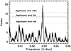 |
Fig. 1 Lomb–Scargle estimate of the power spectrum of all the radial velocity measurements. The lower dotted line corresponds to a false alarm probability of 0.25, dashed line to 0.01, and upper dotted line to 0.001. |
Orbit parameters for the system 2MASS J1808-5104.
4 Stellar parameters
Meléndez et al. (2016) estimated the temperature of 2MASS J1808-5104 by imposing the excitation equilibrium of Fe I lines and adding an empirical correction described in Frebel et al. (2013). Since 2MASS J1808-5104 was observed by Gaia, we used the Gaia photometry recently displayed in the Gaia DR2 (Arenou et al. 2018; Gaia Collaboration 2018), and the 3D maps of interstellar reddening (Capitanio et al. 2017; Lallement et al. 2018; R. Lallement, 2018, priv. comm.) to improve these parameters. The Gaia photometry and the reddening are listed in Table 3. We note that following Schlaufman et al. (2018), the mass of the secondary must be very low (M2 = 0.14 M⊙) and thus its contribution to the total flux is negligible.
In Fig. 3 we compared the position of 2MASS J1808-5104 in a G versus (BP–RP) diagram to the isochrones computed by Chieffi and Limongi (Chieffi & Limongi, 2013, priv. comm.); we used the same code and prescriptions as Straniero et al. (1997) for 12 and 14 Gyr and metallicities of − 3.0 and − 4.0. We note that the error on the G magnitude is very small and is inside the black dot in Fig. 3. The position of the star in the diagram corresponds to a subgiant star with Teff = 5600 K, log g = 3.4, M ≈ 0.8 M⊙, and we decided to adopt this model. As a check we also computed the H α profile for the 1D model adopted by Meléndez (Teff = 5440 K, log g = 3.0) and the model adopted in this work (Teff = 5600 K, log g = 3.4). The fit of the wings of Hα is better with our model. The use of 3D profiles would even point towards a slightly hotter temperature (Amarsi et al. 2018).
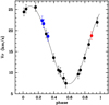 |
Fig. 2 Computed orbit for the 2MASS J1808-5104 system (using the parameters in Table 2) compared with the observedradial velocities based on high resolution spectra. The black points indicate the measurements of Schlaufman et al. (2018). The blue points indicate our measurements based on the UVES R580 spectra given in Table 1. The red point indicates our measurement based on the UVES R760 spectrum as given in Table 1. |
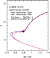 |
Fig. 3 Position of 2MASS J1808-5104 (black dot) in a G vs. (BP–RP) diagram and comparison to isochrones computed by Chieffi and Limongi for very metal-poor stars. |
Photometry and distance of 2MASS J1808-5104 (Gaia DR2 6702907209758894848).
Derived abundances in 2MASS J1808-5104 for Teff = 5600 K, log g = 3.4, vt = 1.6 km s−1 (1D computations, OSMARCS model).
5 Analysis
Since the adopted atmospheric model is rather different from the model adopted by Meléndez et al. (2016), we redetermined the abundances of the different elements with our adopted model. We carried out a classical Local Thermodynamical Equilibrium (LTE) analysis, using OSMARCS models (Gustafsson et al. 1975, 2003, 2008). The abundances were derived using equivalent widths or fits of synthetic spectra when the lines were blended. We used the code turbospectrum (Alvarez & Plez 1998), which includes treatment ofscattering in the blue and UV domains. These abundances are given in Table 4. In Fig. 4, we show the dependence of the iron abundance on the wavelength, excitation potential, and equivalent width of the Fe I line.
-
In Fig. 4b the iron lines with an excitation potential close to zero, over-predict the iron abundance. This is because of non-LTE (NLTE) effects, so these lines are not taken into account in the determination of the mean iron abundance (see Fig. 3 in Cayrel et al. 2004).
-
In Fig. 4c the iron abundance does not depend on the equivalent width of the line, and thus it justifies the choice of the microturbulent velocity, i.e. vt = 1.6 km s−1.
The final 1D, LTE abundances are given in Table 4. The solar abundances are from Caffau et al. (2011) or Lodders et al. (2009).
 |
Fig. 4 Iron abundance from individual lines in 2MASS J1808-5104 as a function of the wavelength, excitation potential, and equivalent width of the line. |
5.1 Carbon and oxygen abundances
In 2MASS J1808-5104, the carbon abundance deduced from the CH band, [C/Fe] = +0.49, is very close to the mean value found from 1D calculations for the extremely metal-poor turn-off stars (Bonifacio et al. 2009): [C/Fe] = +0.45. But the CH band is sensitive to 3D effects (Gallagher et al. 2016). We made use of a 3D CO5BOLD model (Freytag et al. 2012) belonging to the CIFIST grid (Ludwig et al. 2009), with parameters (5500 K/3.5/ − 4.0) close to the stellar parameters of 2MASS J1808-5104 to compute the 3D correction and we found A3D (C) − A1D(C) = −0.40 ± 0.1 dex; the error in this case corresponds to the different estimations of this correction in different parts of the CH band.
The oxygen abundance is derived from a fit of the ultraviolet OH band between 312.2 and 313.2 nm. The uncertainty (scatter from line to line) is less than 0.1 dex. The OH band is also strongly affected by 3D effects. For 12 OH lines, we computed the 3D corrections (Caffau & Ludwig 2007) and we derived A3D (O) − A1D(O) = −0.98 ± 0.08 dex. As a consequence in 2MASS J1808-5104, A(C) = 4.75, [C/H] = − 3.75, [C/Fe] = +0.09 and A(O) = 5.30 with [O/H] = − 3.46 and [O/Fe] = +0.38.
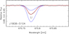 |
Fig. 5 Observed spectrum of 2MASS J1808-5104 in the region of the Li doublet and synthetic spectra computed with A(Li) = 1.5 and 2.1 (blue lines) and 1.78 (red line, best fit). |
5.2 Na and Al abundances
The abundance of these two elements in Table 4 has been deduced from the resonance lines which are often affected by strong NLTE effects. We estimated the NLTE correction from Andrievsky et al. (2007, 2008). In fact the correction at this very low metallicity is small for Na I. We found Δ(A(Na)) = − 0.05, but the correction is large for Al I, i.e. Δ(A(Al)) = +0.68. In 2MASS J1808-5104, the abundances of Na and Al given in Table 4, after correction for NLTE effects, are A(Na) = 2.51, [Na/Fe] = +0.05 and A(Al) = 2.61 and [Al/Fe] = − 0.02
6 Li and Be abundances
The Li abundance is redetermined from our new high S/N spectra in the red (Fig. 5). We find A(Li) = 1.78 a value very close tothe Li abundance found by Meléndez et al. (2016). If we apply the 3D-NLTE correction computed by Sbordone et al. (2010) we find A(Li) = 1.88. As a consequence Li is slightly depleted below the Spite plateau value (Spite & Spite 1982a,b; Sbordone et al. 2010). Lithium indeed is a very fragile element; it is destroyed by proton fusion when temperature reaches about 2 × 10⁶ K. In a main sequence star this element is destroyed as soon as the convective zone reaches the layers where the temperature is higher than this fusion temperature. When the star leaves the main sequence it develops surface convection zones, which deepen as the star evolves to lower temperatures. The surface convection zone mixes the surface layer with deeper material in which lithium has been depleted, and the observed lithium abundance falls. Following Pilachowski et al. (1993), the decrease of Li abundance for Teff = 5600 K is − 0.25 ± 0.25 dex in excellent agreement with the observed Li abundance in 2MASS J1808-5104.
The abundance of Be is determined by a χ2 fit of the observed spectrum (Fig. 6) between 312.94 and 313.14 nm. The best fit depends on the adopted position of the continuum, which is fortunately rather well defined in this region. Only the bluest Be line is used, as is generally done in metal-poor stars, the reddest being much too weak. The Be line at 313.04 nm is close to two OH lines, and to compute the profile of the global feature we use the 1D oxygen abundance given in Table 4. The best fit is obtained for A(Be) = − 2.33, but considering the S/N of the spectrum, it is reasonable to say that A(Be) < − 2.0 or log(Be/H) < − 14.0. Since the weak Be II lines are formed in the deep atmospheric layers, the abundance of Be computed with the 1D-LTE or the 3D-NLTE hypotheses are not significantly different (Primas et al. 2000b).
Although Be is destroyed at a higher temperature than Li (3.5 × 10⁶ K), it is legitimate to ask whether Be has been depleted in 2MASS J1808-5104, since its Li abundance is slightly below the “plateau”. However, we expect that for a same phase of the evolution of the star and thus the same depth of the convective layer, the depletion of Be by dilution is much smaller than the depletion of Li. In the sample of Boesgaard et al. (2011) there is no significant difference between the ratios [Be/Fe] in turn-off and in turn-off and insubgiant stars.
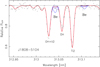 |
Fig. 6 Observed spectrum of 2MASS J1808-5104 in the region of the Be doublet and synthetic spectra computed with A(Be) = − 3.0, − 2.0 and − 1.6 (blue lines), and − 2.33 (red line, best fit). Taking into account the uncertainty in the position of the continuum, we adopted A (Be) ≤−2.0 dex i.e. log (Be/H) ≤−14.0. |
7 Discussion
7.1 Be–Fe correlation
In Fig. 7 we plot log(Be/H) versus [Fe/H] for a large sample of Galactic stars from Smiljanic et al. (2009) and Boesgaard et al. (2011). When a star was in both lists we prefer the abundance given by Smiljanic et al. (2009), but the two are always very close. The black dashed line in Fig. 7 represents the regression line in the middle of these stars.
The two Be measurements at the lowest metallicity are for the stars G 64-12 and G 275-4.
The two Be measurements at the lowest metallicity are for the stars G 64-12 (Primas et al. 2000b; Boesgaard et al. 2011)and G 275-4 (Boesgaard et al. 2011). For G 64-12, Primas et al. (2000b) measure log(Be/H) = − 13.10 ± 0.15, while Boesgaard et al. (2011) found − 13.43 ± 0.12. The two values are compatible within errors, however the difference can be entirely explained by the different atmospheric parameters adopted. Primas et al. (2000b) indeed adopted Teff = 6400 K, log g = 4.1, while Boesgaard et al. (2011) adopted Teff = 6074 K log g = 3.75. This relatively high Be abundance in G 64-12 suggested at that time the possible existence of a “plateau” of the Be abundance at very low metallicity.
As a check we retrieved the UVES and HIRES spectra from the archives. In the region of the Be line, they have almost the same resolution and same S/N so it is possible to average these spectra. The resulting spectrum has a S/N of more than 150 in the region of the Be lines. On this averaged spectrum we remeasured the O and Be abundance in G 64-12 adopting the Primas’s model. The Be abundance is indeed very sensitive to surface gravity and the Gaia DR2 parallax of G 64-12 (3.7626 ± 0.0856) mas implies log g = 4.25; this value is very close to the gravity adopted by Primas et al. (2000b). We found that the best fit was obtained with A(Be) = − 1.35 or log(Be/H) = − 13.35 (Fig. 8). This value is intermediate between the Primas et al. (2000b) and Boesgaard et al. (2011) values. In Fig. 7 the dot representing G 64-12 takes into account this new measurement. The position of the very metal-poor stars G 64-12, G 64-37, and G 275-4 in this figure could suggest the existence of a plateau at a level of log(Be/H) ≈ −13.4.
But before the present work, the most stringent upper limit on the primordial Be abundance was already the upper limit found in the carbon enhanced metal-poor (CEMP) star BD + 44°493 ([Fe/H] = − 3.7) provided by Ito et al. (2009), i.e. log(Be/H) < −14.0. The upper limit that we have derived for 2MASS J1808-5104 is essentially equivalent to that provided by BD + 44°493. The two stars have similar atmospheric parameters and metallicities, however there is a big difference in their carbon and oxygen abundances. With reference to the classification introduced by Bonifacio et al. (2018), while BD + 44°493 is a low-carbon band CEMP star, 2MASS J1808-5104 is a carbon normal star. This finding confirms what was already noticed by Ito et al. (2009): there is no correlation between CEMP nature and Be abundance.
The very low abundances of Be in 2MASS J1808-5104 confirms that the possibility of a Be plateau at a level of log(Be/H) ≈ − 13.6 is ruled out (Fig 7). It seems reasonable to assume that the Be abundance continues its linear decrease with metallicity in the range − 3.0 to − 4.0 dex. We found that, on average, log (Be∕H) = −10.75 + 0.89 *[Fe/H] (see dashed line in Fig. 7). The slope of this line is very close to the slope found by Boesgaard et al. (2011) from their stars alone. The low Be abundance found in 2MASS J1808-5104 and BD + 44°493 is compatible with this linear regression.
The upper limit on the primordial Be abundance log(Bep/H) < −14 is thus reinforced as are the limits on late decaying hadrons provided by Pospelov & Pradler (2011). At present there appears to be no hint towards inhomogeneities in the primordial plasma or the presence of late decaying particles.
 |
Fig. 7 For galactic stars, log(Be/H) vs. [Fe/H]. The green open circles are from Smiljanic et al. (2009) and the blue filled circles from Boesgaard et al. (2011). However the position of G 64-12 in this diagram takes into account our new measurement of the Be abundance in this star adopting the model of Primas et al. (2000b), which is in better agreement with the Gaia-DR2 data. The upper limit of the abundance of Be in 2MASS J1808-5104 and BD + 44°493 are indicated with big red and blue open circles. The blue dashed straight line represents the mean relation. The curved red dash-dotted line at low metallicity represents the possibility of a plateau, suggested in particular, by the previous high Be abundance found in G 64-12 by Primas et al. (2000b) and Boesgaard et al. (2011). The very low Be abundance in the two additional stars BD + 44°493 and 2MASS J1808-5104 rules out the possibility of a plateau. |
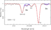 |
Fig. 8 Mean of the reduced G64-12 spectra obtained with the HIRES-Keck and the UVES-VLT spectrographs in the region of the Be doublet and synthetic spectra computed with A(Be) = − 3.0, − 1.5, − 1.2 (blue lines), and − 1.35 (red line, best fit). |
7.2 Be–O correlation
In Fig. 9 we plot log(Be/H) as a function of [O/H] for the stars studied by Boesgaard et al. (2011) in which the oxygen abundance was deduced from 1D computations of the profile of some UV–OH lines; the authors estimated that the error in [O/H] is about 0.2 dex. As discussed in Sect. 5.1, these lines are strongly affected by 3D effects. The 3D correction has been computed by Asplund & García Pérez (2001) and González Hernández et al. (2010) with two different grids of 3D models and their results are in good agreement. For dwarfs and subgiant stars this correction depends mainly on the metallicity and temperature of the star; this correction is negligible for [Fe∕H] > −1.0 but reaches almost − 1.0 for [Fe∕H] = −4.0.
The starBD + 44°493 is peculiar, it is very C-rich and Gallagher et al. (2017) have shown that the carbon abundance affects the molecular equilibria in 3D hydrodynamical models in a much more prominent way than happens in 1D models. Using a C-rich hydrodynamical model atmosphere computed with the CO5BOLD code (Freytag et al. 2012), we determined that the 3D correction in this case is only − 0.3 dex. As a consequence [O/H] in BD + 44°493 is equal to − 2.49.
The OH lines can be also affected by NLTE effects. Asplund & García Pérez (2001) approximated the UV–OH line formation with a two-level approach with complete redistribution, but they neglected the influence of NLTE on the dissociation of the molecules. These authors found from 1D computations that the oxygen abundance derived from the UV–OH band is underestimated by about 0.2 dex, almost independently from the stellar parameters. In order to obtain a right estimation of the NLTE effect it would be necessary to take into account fully the 3D thermal structure of the model atmosphere; this work is beyond the scope of this paper.
To date, we neglected the NLTE correction and we applied to all the stars of the sample of Boesgaard et al. (2011) the 3D correction computed from González Hernández et al. (2010).
In Fig. 9A the oxygen abundance was computed from 1D models (as in Boesgaard et al. 2011) and in Fig. 9B, this oxygen abundance was corrected for 3D effects. If we had applied the Asplund & García Pérez (2001) NLTE correction, all the dots in Fig. 9B would have been shifted by 0.2 dex towards higher [O/H] values.
When only Boesgaard’s stars are considered, the data after 3D correction can be interpreted by a linear relation between log(Be/H) and [O/H] with a slope of 0.77. Alternatively a two-slope relation (see Boesgaard et al. 2011) with a slope of 0.95 in the interval − 1.5 < [O/H] < 0.0 and a slope of 0.58 at lower metallicity can be used.
In Fig. 9A or B, 2MASS J1808-5104 and BD + 44°493 do not fit the general trend. The star BD + 44°493 has an oxygen abundance close to the oxygen abundance of G 64-12, and 2MASS J1808-5104 has about the same as G 275-4 and G 64-37, but 2MASS J1808-5104 like BD + 44°493 are clearly more deficient in Be. The Be abundance expected in 2MASS J1808-5104, from the mean relations in Fig. 9, would be in all the cases A(Be) ≈ −1.6, a value excluded from the observed spectrum (see Fig. 6).
Since BD + 44°493 is a C-rich star it could be possible that the high CNO abundances in this star are the result of a mass transfer from a “now dead” AGB companion. But since the star is a CEMP-no (no enrichment of the neutron capture elements) this interpretation is unlikely. Moreover, following Gaia Collaboration (2018), the radial velocity of BD + 44°493 does not seem variable, i.e. RV = − 147.9. As a consequence, the existence of a former pollution of the atmosphere of BD + 44°493 by a massive companion in its AGB phase is questionable. It is highly probable that the abundance of C, N and O in the atmosphere of BD + 44°493 is a good witness of the abundances in the cloud which formed the star.
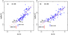 |
Fig. 9 For galactic stars, log(Be/H) vs. [O/H] following Boesgaard et al. (2011; blue filled circles). The upper limit of the abundance of Be in 2MASS J1808-5104 and BD + 44°493 are indicated with big red and blue open circles. Panel A: the oxygen abundance was simply computed with the 1D LTE hypothesis, as in Boesgaard et al. (2011). Panel B: this abundance has been corrected for 3D effects. The blue dashed line represents the mean relation and the red dashed line the two-slope solution with a change of the slope around [O/H] = − 1.5 dex as in Boesgaard et al. (2011). The positions of BD + 44°493 and 2MASS J1808-5104 in this diagram are hardly compatible with the mean relations. |
8 Conclusions
A two-slope solution of the relation log(Be/H) versus [O/H] is predicted by theory. It is now commonly accepted that all the observed Be is formed by spallation (Reeves et al. 1970; Meneguzzi et al. 1971), however the following two distinct processes can be invoked:
-
H and He nuclei in cosmic rays hit CNO nuclei in the ambient interstellar gas (secondary process).
-
CNO nuclei in the cosmic rays hit H and He nuclei in the ambient interstellar gas (primary process).
If Be (and B) were formed preferentially by the secondary process we would expect a quadratic dependence of the Be (B) abundance on the oxygen abundance, hence a slope of two in the logarithmic plane. The primary process, on the other hand, would imply a slope of one, as implied by the observations of both Be and B. The secondary process was probably invoked for the first time as the main process for the production of B (and Be by extension) by Duncan et al. (1992) to explain their B observations. Further considerations on this point can be found in Duncan (1997); Molaro et al. (1997) and Rich & Boesgaard (2009). However, from the theoretical point of view Suzuki et al. (1999) and Suzuki & Yoshii (2001) argued that the primary process is the main source of all the observed B and Be.
Boesgaard et al. (2011) suggested that the balance shifted from primary to secondary in the course of time. In the early days of Galactic evolution, the acceleration of CNO atoms from SNe II should be the main phenomenon and the number of Be atoms should be proportional to the number of SNe II and thus to the number of O atoms. Later the number of O atoms is proportional to the cumulative number of SN II, while the energetic protons are proportional to the instantaneous number of SN II. As a consequence the slope of the relation log(Be/H) versus [O/H] is expected to change, and for this reason Boesgaard et al. (2011) tried to describe the Galactic evolution of Be with two straight lines and a break at a metallicity around − 1.5. The slopes of the different relations in Fig. 9B are slightly different from those of Boesgaard et al. (2011) since we correct the abundance of oxygen for 3D effects.
In Bonifacio et al. (2015) we argued that low-carbon band CEMP stars, such as BD + 44°493, were formed from gas that was polluted by SNe that experienced a large fall-back of material onto the compact remnant, resulting in very high ratios of CNO elements to iron. We referred to these as “faint supernovae” (SNe) because we made the implicit assumption that the luminosities of these stars would also be lower than those of SNe that do not experience fall-back. Observationally this same name is given to type II SNe that are under-luminous, such as SN 1997D (de Mello et al. 1997), which was also characterised by relatively low expansion velocities and a low mass of ejected 56Ni (Turatto et al. 1998). It is interesting to note that SN 1997D should not have been able to produce light elements via spallation. The cross section for production of 9Be via spallation of oxygen drops drastically below energies of a few (MeV/A) of the projectile (see Fig. 1 of Suzuki & Yoshii 2001), and, translated into velocity of the O nuclei, this requires velocities in excess of 4000 km s−1. A typical type II SNe shows velocities of the ejecta that are of the order of 10 000 km s−1, thus in the useful range for Be production. On the other hand SN 1997D showed an expansion velocity of the ejecta of only 1200 km s−1 (Turatto et al. 1998), which is clearly insufficient for Be production. The upper limit of BD + 44°493 seems to be consistent with the hypothesis that it was formed from a faint SNe, characterised by strong fall-back, responsible for the high CNO to Fe ratios, and low velocity of the ejecta, resulting in a Be content that is clearly lower than that of stars of similar [O/H]. In fact it could well be that BD + 44°493 is completely devoid of Be, and that the fact that its upper limit on its Be abundance falls exactly on the expected line of Be–Fe evolution, is fortuitous. It would be of paramount importance to be able to push down the upper limit on the abundance of Be in BD + 44°493, even by only 0.3 dex. As a corollary, measurements of Be in other lower carbon CEMP unevolved stars are strongly encouraged. If our scenario is correct, all lower carbon CEMP unevolved stars should show a lower Be abundance than carbon-normal stars of similar [O/H]. The unevolved lower carbon band CEMP star, HE 1327-2326, has an upper limit on the Be abundance log (Be/H) < −13.2 and a 3D corrected [O/H] = − 2.64 (Frebel et al. 2008, for this star the 3D correction is − 0.72 dex). This upper limit is inconclusive since it is above the Be abundance measured in stars of comparable O abundance, and also above both the two-slope model and the one-slope model. It would be extremely important to be able to push down this upper limit by 0.3–0.4 dex. A detection of Be at the same level as that in stars of similar O abundance would invalidate our scenario on faint SNe.
While the low Be abundance in BD + 44°493 could be interpreted as a result of it being formed from ejecta of a faint SNe, the same cannot be invoked for 2MASS J1808-5104. As we have already argued, the Li abundance measured in 2MASS J1808-5104 is strong evidence that the Be in this star cannot have been significantly depleted. The fact that there are stars that have similar oxygen abundances but significantly different Be abundances is a real puzzle. A fundamental piece of information would, of course, come from a measure of the Be abundance in 2MASS J1808-5104, or at least an upper limit lower by 0.3 dex. This would at least ruleout the possibility that the difference is simply due to large observational errors in both Be and O abundances. A far more intriguing possibility is that in the early Galaxy, the tight correlation of Be with O breaks down: the scatter of the relation becomes larger. In a simple picture, 2MASS J1808-5104 and BD + 44°493 should be very old stars born in regions with anomalously high O, due to local inhomogeneities in the very early Galaxy.
Given the very low metallicity of 2MASS J1808-5104 we may assume that the SNe, that have produced the metals that we observe in its atmosphere, were Pop III stars, possibly even a single Pop III star or a few at most. If the velocities of the ejecta in these stars were higher than observed in normal Pop I and Pop II SNe, it may be that the lower mass spallation products, Li, Be and B, escape with a high enough velocity to escape the cloud that will give rise to the next generation of stars, such as 2MASS J1808-5104. If this were the case, we expect that stars at the metallicity of 2MASS J1808-5104 ([Fe/H] ≤ −3.5) are all devoid of Be and B.
This would also be an interesting diagnostic to distinguish true descendants of Pop III stars from stars of similar metallicity, but formed from clouds polluted by Pop II stars. This clearly prompts for new observations: on the one hand, it is important to measure Be and B in 2MASS J1808-5104 and other stars of similarly low metallicity and, on the other hand, one should increase the number of stars with measured Be and B in the metallicity range [Fe/H] ≤−2.0. A single or a few Pop III SNe can pollute a gas cloud to such high metallicities and a measure of Be could allow us to detect such true Pop IIIdescendants.
Acknowledgements
A.J.G. would like to acknowledge support by Sonderforschungsbereich SFB 881 “The Milky Way System” (subproject A5) of the German Research Foundation (DFG). This work uses results from the European Space Agency (ESA) space mission Gaia. Gaia data are being processed by the Gaia Data Processing and Analysis Consortium (DPAC). Funding for the DPAC is provided by national institutions, in particular the institutions participating in the Gaia MultiLateral Agreement (MLA). The Gaia mission website is https://www.cosmos.esa.int/gaia. The Gaia archive website is https://archives.esac.esa.int/gaia.
Note added in proof. The relation between Be and Fe found in Sect. 7.1 is almost identical to the predictions of the model b of Vangioni-Flam et al. (1998). In this model, Be is produced by standard GCR from ejecta of individual SN II with progenitors in the same mass range as that responsible for Fe production (M > 8 M⊙).
References
- Alvarez, R., & Plez, B. 1998, A&A, 330, 1109 [NASA ADS] [Google Scholar]
- Amarsi, A. M., Nordlander, T., Barklem, P. S., et al. 2018, A&A, 615, A139 [NASA ADS] [CrossRef] [EDP Sciences] [Google Scholar]
- Andrievsky, S. M., Spite, M., Korotin, S. A., et al. 2007, A&A, 464, 1081 [NASA ADS] [CrossRef] [EDP Sciences] [Google Scholar]
- Andrievsky, S. M., Spite, M., Korotin, S. A., et al. 2008, A&A, 481, 481 [NASA ADS] [CrossRef] [EDP Sciences] [Google Scholar]
- Arenou, F., Luri, X., Babusiaux, C., et al. 2018, A&A, 616, A17 [Google Scholar]
- Asplund, M. 2004, A&A, 417, 769 [NASA ADS] [CrossRef] [EDP Sciences] [Google Scholar]
- Asplund, M., & García Pérez, A. E. 2001, A&A, 372, 601 [NASA ADS] [CrossRef] [EDP Sciences] [Google Scholar]
- Balachandran, S. C., & Bell, R. A. 1998, Nature, 392, 791 [NASA ADS] [CrossRef] [Google Scholar]
- Ballester, P., Modigliani, A., Boitquin, O., et al. 2000, The Messenger, 101, 31 [NASA ADS] [Google Scholar]
- Beers, T. C., Suzuki, T. K., & Yoshii, Y. 2000, The Light Elements and their Evolution, IAU Symp., 198, 425 [NASA ADS] [Google Scholar]
- Boesgaard, A. M. 1976, ApJ, 210, 466 [NASA ADS] [CrossRef] [Google Scholar]
- Boesgaard, A. M. 2007, ApJ, 667, 1196 [NASA ADS] [CrossRef] [Google Scholar]
- Boesgaard, A. M., & King, J. R. 1993, AJ, 106, 2309 [NASA ADS] [CrossRef] [Google Scholar]
- Boesgaard, A. M., & King, J. R. 2002, ApJ, 565, 587 [NASA ADS] [CrossRef] [Google Scholar]
- Boesgaard, A. M., Deliyannis, C. P., King, J. R., et al. 1999, AJ, 117, 1549 [NASA ADS] [CrossRef] [Google Scholar]
- Boesgaard, A. M., Rich, J. A., Levesque, E. M., & Bowler, B. P. 2011, ApJ, 743, 140 [NASA ADS] [CrossRef] [Google Scholar]
- Bonifacio, P., Spite, M., Cayrel, R., et al. 2009, A&A, 501, 519 [NASA ADS] [CrossRef] [EDP Sciences] [Google Scholar]
- Bonifacio, P., Caffau, E., Spite, M., et al. 2015, A&A, 579, A28 [NASA ADS] [CrossRef] [EDP Sciences] [Google Scholar]
- Bonifacio, P., Caffau, E., Spite, M., et al. 2018, A&A, 612, A65 [NASA ADS] [CrossRef] [EDP Sciences] [Google Scholar]
- Boyd, R. N., & Kajino, T. 1989, ApJ, 336, L55 [NASA ADS] [CrossRef] [Google Scholar]
- Caffau, E., & Ludwig, H.-G. 2007, A&A, 467, L11 [NASA ADS] [CrossRef] [EDP Sciences] [Google Scholar]
- Caffau, E., Ludwig, H.-G., Steffen, M., Freytag, B., & Bonifacio, P. 2011, Sol. Phys., 268, 255 [NASA ADS] [CrossRef] [Google Scholar]
- Capitanio, L., Lallement, R., Vergely, J. L., Elyajouri, M., & Monreal-Ibero, A. 2017, A&A, 606, A65 [NASA ADS] [CrossRef] [EDP Sciences] [Google Scholar]
- Carlberg, J. K., Cunha, K., Smith, V. V., & do Nascimento, J.-D., Jr. 2018, ApJ, 865, 8 [NASA ADS] [CrossRef] [Google Scholar]
- Cayrel, R., Depagne, E., Spite, M., et al. 2004, A&A, 416, 1117 [NASA ADS] [CrossRef] [EDP Sciences] [Google Scholar]
- Chmielewski, Y., Brault, J. W., & Mueller, E. A. 1975, A&A, 42, 37 [NASA ADS] [Google Scholar]
- Dekker, H., D’Odorico, S., Kaufer, A., Delabre, B., & Kotzlowski, H. 2000, Proc. SPIE, 4008, 534 [Google Scholar]
- de Mello, D., Benetti, S., & Massone, G. 1997, IAU Circ., 6537, 1 [NASA ADS] [Google Scholar]
- Duncan, D. K. 1997, Nucl. Phys. A, 621, 10 [NASA ADS] [CrossRef] [Google Scholar]
- Duncan, D. K., Lambert, D. L., & Lemke, M. 1992, ApJ, 401, 584 [NASA ADS] [CrossRef] [Google Scholar]
- Frebel, A., Collet, R., Eriksson, K., Christlieb, N., & Aoki, W. 2008, ApJ, 684, 588 [NASA ADS] [CrossRef] [Google Scholar]
- Frebel, A., Casey, A. R., Jacobson, H. R., & Yu, Q. 2013, ApJ, 769, 57 [NASA ADS] [CrossRef] [Google Scholar]
- Freytag, B., Steffen, M., Ludwig, H.-G., et al. 2012, J. Comput. Phys., 231, 919 [Google Scholar]
- Gaia Collaboration (Brown, A. G. A., et al.) 2018, A&A, 616, A1 [NASA ADS] [CrossRef] [EDP Sciences] [Google Scholar]
- Gallagher, A. J., Caffau, E., Bonifacio, P., et al. 2016, A&A, 593, A48 [NASA ADS] [CrossRef] [EDP Sciences] [Google Scholar]
- Gallagher, A. J., Caffau, E., Bonifacio, P., et al. 2017, A&A, 598, L10 [NASA ADS] [CrossRef] [EDP Sciences] [Google Scholar]
- Gilmore, G., Edvardsson, B., & Nissen, P. E. 1991, ApJ, 378, 17 [NASA ADS] [CrossRef] [Google Scholar]
- Gilmore, G., Gustafsson, B., Edvardsson, B., & Nissen, P. E. 1992, Nature, 357, 379 [NASA ADS] [CrossRef] [Google Scholar]
- González Hernández, J. I., Bonifacio, P., Ludwig, H.-G., et al. 2010, A&A, 519, A46 [NASA ADS] [CrossRef] [EDP Sciences] [Google Scholar]
- Gustafsson, B., Bell, R. A., Eriksson, K., Nordlund, Å., 1975, A&A, 42, 407 [Google Scholar]
- Gustafsson, B., Edvardsson, B., Eriksson, K., et al. 2003, in Stellar Atmosphere Modeling, eds. I. Hubeny, D. Mihalas, & K. Werner, ASP Conf. Ser., 288, 331 [Google Scholar]
- Gustafsson, B., Edvardsson, B., Eriksson, K., et al. 2008, A&A, 486, 951 [NASA ADS] [CrossRef] [EDP Sciences] [Google Scholar]
- Ito, H., Aoki, W., Honda, S., & Beers, T. C. 2009, ApJ, 698, L37 [NASA ADS] [CrossRef] [Google Scholar]
- Jacquinet-Husson, N., Scott, N. A., Chédin, A., et al. 2005, J. Quant. Spectr. Rad. Transf., 95, 429 [NASA ADS] [CrossRef] [Google Scholar]
- Jedamzik, K. 2006, Phys. Rev. D, 74, 103509 [NASA ADS] [CrossRef] [Google Scholar]
- Kusakabe, M., Kajino, T., Yoshida, T., & Mathews, G. J. 2009, Phys. Rev. D, 80, 103501 [CrossRef] [Google Scholar]
- Lallement, R., Capitanio, L., Ruiz-Dern, L., et al. 2018, A&A, 616, A132 [NASA ADS] [CrossRef] [EDP Sciences] [Google Scholar]
- Lodders, K., Palme, H., & Gail, H.-P. 2009, in Landolt Börnstein, New Series Astronomy and Astrophysics, ed. J. E. Trümper (Berlin: Springer Verlag), VI/4B, 560 [Google Scholar]
- Lomb, N. R. 1976, Ap&SS, 39, 447 [Google Scholar]
- Ludwig, H.-G., Caffau, E., Steffen, M., et al. 2009, Mem. Soc. Astron. It., 80, 711 [Google Scholar]
- Meléndez, J., Placco, V. M., Tucci-Maia, M., et al. 2016, A&A, 585, L5 [NASA ADS] [CrossRef] [EDP Sciences] [Google Scholar]
- Meneguzzi, M., Audouze, J., & Reeves, H. 1971, A&A, 15, 337 [NASA ADS] [Google Scholar]
- Molaro, P. 1987, Ph.D. Thesis, SISSA, Trieste, Italy [Google Scholar]
- Molaro, P., & Beckman, J. 1984, A&A, 139, 394 [NASA ADS] [Google Scholar]
- Molaro, P., Bonifacio, P., Castelli, F., & Pasquini, L. 1997, A&A, 319, 593 [NASA ADS] [Google Scholar]
- Molaro, P., Levshakov, S. A., Monai, S., et al. 2008, A&A, 481, 559 [NASA ADS] [CrossRef] [EDP Sciences] [Google Scholar]
- Nave, G., Johansson, S., Learner, R. C. M., Thorne, A. P., & Brault, J. W. 1994, ApJS, 94, 221 [NASA ADS] [CrossRef] [Google Scholar]
- Pasquini, L., Bonifacio, P., Randich, S., Galli, D., & Gratton, R. G. 2004, A&A, 426, 651 [NASA ADS] [CrossRef] [EDP Sciences] [Google Scholar]
- Pasquini, L., Galli, D., Gratton, R. G., et al. 2005, A&A, 436, L57 [NASA ADS] [CrossRef] [EDP Sciences] [Google Scholar]
- Pasquini, L., Bonifacio, P., Randich, S., et al. 2007, A&A, 464, 601 [NASA ADS] [CrossRef] [EDP Sciences] [Google Scholar]
- Pilachowski, C. A., Sneden, C., & Booth, J. 1993, ApJ, 407, 699 [NASA ADS] [CrossRef] [Google Scholar]
- Pitrou, C., Coc, A., Uzan, J.-P., & Vangioni, E. 2018, Phys. Rep., 754, 1 [NASA ADS] [CrossRef] [Google Scholar]
- Placco, V. M., Beers, T. C., Reggiani, H., & Meléndez, J. 2016, ApJ, 829, L24 [NASA ADS] [CrossRef] [Google Scholar]
- Pospelov, M., & Pradler, J. 2011, Phys. Rev. Lett., 106, 121305 [NASA ADS] [CrossRef] [Google Scholar]
- Primas, F., Molaro, P., Bonifacio, P., & Hill, V. 2000a, A&A, 362, 666 [NASA ADS] [Google Scholar]
- Primas, F., Asplund, M., Nissen, P. E., & Hill, V. 2000b, A&A, 364, L42 [NASA ADS] [Google Scholar]
- Reeves, H., Fowler, W.A., & Hoyle, F. 1970, Nature, 226, 727 [NASA ADS] [CrossRef] [PubMed] [Google Scholar]
- Rebolo, R., Molaro, P., Abia, C., & Beckman, J. E. 1988, A&A, 193, 193 [NASA ADS] [Google Scholar]
- Rich, J. A., & Boesgaard, A. M. 2009, ApJ, 701, 1519 [NASA ADS] [CrossRef] [Google Scholar]
- Roederer, I. U., Karakas, A. I., Pignatari, M., & Herwig, F. 2016, ApJ, 821, 37 [NASA ADS] [CrossRef] [Google Scholar]
- Ryan, S. G., Norris, J. E., Bessell, M. S., & Deliyannis, C. 1992, ApJ, 388, 184 [NASA ADS] [CrossRef] [Google Scholar]
- Sartoretti, P., Katz, D., Cropper, M., et al. 2018, A&A, 616, A6 [NASA ADS] [CrossRef] [EDP Sciences] [Google Scholar]
- Sbordone, L., Bonifacio, P., Caffau, E., et al. 2010, A&A, 522, A26 [NASA ADS] [CrossRef] [EDP Sciences] [Google Scholar]
- Scargle, J. D. 1982, ApJ, 263, 835 [Google Scholar]
- Schlaufman, K. C., Thompson, I. B., & Casey, A. R. 2018, ApJ, 867, 98 [NASA ADS] [CrossRef] [Google Scholar]
- Smiljanic, R., Pasquini, L., Bonifacio, P., et al. 2009, A&A, 499, 103 [NASA ADS] [CrossRef] [EDP Sciences] [Google Scholar]
- Spite, M., & Spite, F. 1982a, Nature, 297, 483 [NASA ADS] [CrossRef] [Google Scholar]
- Spite, F., & Spite, M. 1982b, A&A, 115, 357 [NASA ADS] [Google Scholar]
- Straniero, O., Chieffi, A., & Limongi, M. 1997, ApJ, 490, 425 [NASA ADS] [CrossRef] [Google Scholar]
- Suzuki, T. K., & Yoshii, Y. 2001, ApJ, 549, 303 [NASA ADS] [CrossRef] [Google Scholar]
- Suzuki, T. K., Yoshii, Y., & Kajino, T. 1999, ApJ, 522, L125 [NASA ADS] [CrossRef] [Google Scholar]
- Tan, K., & Zhao, G. 2011, ApJ, 738, L33 [NASA ADS] [CrossRef] [Google Scholar]
- Tan, K. F., Shi, J. R., & Zhao, G. 2009, MNRAS, 392, 205 [NASA ADS] [CrossRef] [Google Scholar]
- Turatto, M., Mazzali, P. A., Young, T. R., et al. 1998, ApJ, 498, L129 [NASA ADS] [CrossRef] [Google Scholar]
- Vangioni-Flam, E., Ramaty, R., Olive, K. A., & Casse, M. 1998, A&A, 337, 714 [NASA ADS] [Google Scholar]
- Wichmann, R., Schmitt, J. H. M. M., & Hubrig, S. 2003, A&A, 400, 293 [NASA ADS] [CrossRef] [EDP Sciences] [Google Scholar]
All Tables
Derived abundances in 2MASS J1808-5104 for Teff = 5600 K, log g = 3.4, vt = 1.6 km s−1 (1D computations, OSMARCS model).
All Figures
|
Fig. 1 Lomb–Scargle estimate of the power spectrum of all the radial velocity measurements. The lower dotted line corresponds to a false alarm probability of 0.25, dashed line to 0.01, and upper dotted line to 0.001. |
| In the text | |
|
Fig. 2 Computed orbit for the 2MASS J1808-5104 system (using the parameters in Table 2) compared with the observedradial velocities based on high resolution spectra. The black points indicate the measurements of Schlaufman et al. (2018). The blue points indicate our measurements based on the UVES R580 spectra given in Table 1. The red point indicates our measurement based on the UVES R760 spectrum as given in Table 1. |
| In the text | |
|
Fig. 3 Position of 2MASS J1808-5104 (black dot) in a G vs. (BP–RP) diagram and comparison to isochrones computed by Chieffi and Limongi for very metal-poor stars. |
| In the text | |
|
Fig. 4 Iron abundance from individual lines in 2MASS J1808-5104 as a function of the wavelength, excitation potential, and equivalent width of the line. |
| In the text | |
|
Fig. 5 Observed spectrum of 2MASS J1808-5104 in the region of the Li doublet and synthetic spectra computed with A(Li) = 1.5 and 2.1 (blue lines) and 1.78 (red line, best fit). |
| In the text | |
|
Fig. 6 Observed spectrum of 2MASS J1808-5104 in the region of the Be doublet and synthetic spectra computed with A(Be) = − 3.0, − 2.0 and − 1.6 (blue lines), and − 2.33 (red line, best fit). Taking into account the uncertainty in the position of the continuum, we adopted A (Be) ≤−2.0 dex i.e. log (Be/H) ≤−14.0. |
| In the text | |
|
Fig. 7 For galactic stars, log(Be/H) vs. [Fe/H]. The green open circles are from Smiljanic et al. (2009) and the blue filled circles from Boesgaard et al. (2011). However the position of G 64-12 in this diagram takes into account our new measurement of the Be abundance in this star adopting the model of Primas et al. (2000b), which is in better agreement with the Gaia-DR2 data. The upper limit of the abundance of Be in 2MASS J1808-5104 and BD + 44°493 are indicated with big red and blue open circles. The blue dashed straight line represents the mean relation. The curved red dash-dotted line at low metallicity represents the possibility of a plateau, suggested in particular, by the previous high Be abundance found in G 64-12 by Primas et al. (2000b) and Boesgaard et al. (2011). The very low Be abundance in the two additional stars BD + 44°493 and 2MASS J1808-5104 rules out the possibility of a plateau. |
| In the text | |
|
Fig. 8 Mean of the reduced G64-12 spectra obtained with the HIRES-Keck and the UVES-VLT spectrographs in the region of the Be doublet and synthetic spectra computed with A(Be) = − 3.0, − 1.5, − 1.2 (blue lines), and − 1.35 (red line, best fit). |
| In the text | |
|
Fig. 9 For galactic stars, log(Be/H) vs. [O/H] following Boesgaard et al. (2011; blue filled circles). The upper limit of the abundance of Be in 2MASS J1808-5104 and BD + 44°493 are indicated with big red and blue open circles. Panel A: the oxygen abundance was simply computed with the 1D LTE hypothesis, as in Boesgaard et al. (2011). Panel B: this abundance has been corrected for 3D effects. The blue dashed line represents the mean relation and the red dashed line the two-slope solution with a change of the slope around [O/H] = − 1.5 dex as in Boesgaard et al. (2011). The positions of BD + 44°493 and 2MASS J1808-5104 in this diagram are hardly compatible with the mean relations. |
| In the text | |
Current usage metrics show cumulative count of Article Views (full-text article views including HTML views, PDF and ePub downloads, according to the available data) and Abstracts Views on Vision4Press platform.
Data correspond to usage on the plateform after 2015. The current usage metrics is available 48-96 hours after online publication and is updated daily on week days.
Initial download of the metrics may take a while.