| Issue |
A&A
Volume 623, March 2019
|
|
|---|---|---|
| Article Number | A113 | |
| Number of page(s) | 20 | |
| Section | Numerical methods and codes | |
| DOI | https://doi.org/10.1051/0004-6361/201834642 | |
| Published online | 13 March 2019 | |
A physical approach to modelling large-scale galactic magnetic fields
1
School of Mathematics, Statistics and Physics, Newcastle University, Newcastle upon Tyne NE1 7RU, UK
e-mail: This email address is being protected from spambots. You need JavaScript enabled to view it.
, This email address is being protected from spambots. You need JavaScript enabled to view it.
, This email address is being protected from spambots. You need JavaScript enabled to view it.
2
Department of Astrophysics/IMAPP, Radboud University, PO Box 9010, 6500 GL Nijmegen, The Netherlands
Received:
14
November
2018
Accepted:
22
January
2019
Abstract
Context. A convenient representation of the structure of the large-scale galactic magnetic field is required for the interpretation of polarization data in the sub-mm and radio ranges, in both the Milky Way and external galaxies.
Aims. We develop a simple and flexible approach to construct parametrised models of the large-scale magnetic field of the Milky Way and other disc galaxies, based on physically justifiable models of magnetic field structure. The resulting models are designed to be optimised against available observational data.
Methods. Representations for the large-scale magnetic fields in the flared disc and spherical halo of a disc galaxy were obtained in the form of series expansions whose coefficients can be calculated from observable or theoretically known galactic properties. The functional basis for the expansions is derived as eigenfunctions of the mean-field dynamo equation or of the vectorial magnetic diffusion equation.
Results. The solutions presented are axially symmetric but the approach can be extended straightforwardly to non-axisymmetric cases. The magnetic fields are solenoidal by construction, can be helical, and are parametrised in terms of observable properties of the host object, such as the rotation curve and the shape of the gaseous disc. The magnetic field in the disc can have a prescribed number of field reversals at any specified radii. Both the disc and halo magnetic fields can separately have either dipolar or quadrupolar symmetry. The model is implemented as a publicly available software package GALMAG which allows, in particular, the computation of the synchrotron emission and Faraday rotation produced by the model’s magnetic field.
Conclusions. The model can be used in interpretations of observations of magnetic fields in the Milky Way and other spiral galaxies, in particular as a prior in Bayesian analyses. It can also be used for a simple simulation of a time-dependent magnetic field generated by dynamo action.
Key words: Galaxy: general / galaxies: spiral / magnetic fields / dynamo / polarization
© ESO 2019
1. Introduction
Recent increased interest in the large-scale magnetic fields of the Milky Way (MW) and other spiral galaxies is driven by a number of factors. Their role in the dynamics of the interstellar medium (ISM) has been widely appreciated although not completely understood. Their significance for the feedback processes in evolving galaxies has also been recognised and is being actively explored (e.g. Hopkins et al. 2018). Furthermore, the separation of the Galactic foreground, including its magnetic field and associated emission, from extragalactic contributions is essential to identify the sources of ultra-high energy cosmic rays (UHECR; Kotera & Olinto 2011; Mollerach & Roulet 2018) and for cosmological interpretations of sensitive CMB observations (e.g. Planck Collaboration XI 2019).
Our understanding of the Galactic magnetic field (GMF) is based on observations of Faraday rotation of polarised radio emission, synchrotron emission of energetic electrons, and polarised emission and absorption by dust (e.g. Haverkorn 2015). Observations of external spiral galaxies have provided rich polarisation data for their discs and haloes (Beck 2015; Wiegert et al. 2015; Mao et al. 2015). Interpretation of such data in terms of three-dimensional magnetic field structures requires parametrised models of the magnetic field based on the understanding of their nature and origin. It can be expected that models that rely less on specific theoretical models would have a larger number of free parameters whose physical meaning would be less clear. On the contrary, physically motivated models can be more flexible and lead to physically transparent interpretations of observations.
A range of heuristic models for the structure of the GMF have been proposed (e.g. Sun et al. 2008; Jaffe et al. 2010; Van Eck et al. 2011; Jansson & Farrar 2012a,b; Ferrière & Terral 2014; Terral & Ferrière 2017). Magnetic fields in most of these models are superpositions of various ad hoc parts whose parameters are selected by fitting to a range of observables. The heuristic nature of the models makes them rather inflexible. Furthermore, their parameters are not necessarily related to the ISM properties (often lacking a transparent physical meaning), and some such models fail to satisfy even such fundamental constraints as ∇ ⋅ B = 0 or to allow for the global helical nature of galactic magnetic fields that imprints on its structure and symmetries. The ambiguities, problems and limitations of the current approaches to GMF modelling have been discussed in Planck Collaboration XLII (2016) and by the IMAGINE consortium (Boulanger et al. 2018).
A possible way to overcome heuristics in GMF modelling would be to extract the field structure from physical simulations of galaxy formation and evolution, which include all relevant processes of magnetic field generation and are specific to the MW. Such simulations of generic galaxies have led to important insights into various magnetic structures in spiral galaxies (e.g. Pakmor et al. 2017; Pakmor & Springel 2013) but their resolution remains insufficient to capture galactic dynamo action, as it is controlled by turbulent processes on scales less than 100 pc. Moreover, the simulations would have to be constrained in a way flexible enough to reproduce an ever increasing set of observational data.
Here we propose a simple (that is, flexible, adjustable, analytic) and yet realistic (i.e., based on relevant equations and observations) approach to model the large-scale (mean) magnetic field in the disc and halo of the Milky Way and other spiral galaxies. The model has been implemented as a publicly available software package GALMAG (Rodrigues 2018), which can be used in the framework of Bayesian optimisers (e.g. Steininger et al. 2018; Steininger 2018).
The text is organised as follows. In Sect. 2, we lay out the modelling strategy, basic equations and fundamental assumptions. In Sect. 3, we describe the solutions for magnetic field in the disc and in Sect. 4, for the halo. In Sect. 5 we discuss possible applications of this model to the interpretation of observations of synchrotron emission and Faraday rotation (Sect. 5.1) as well some of the ways in which it could be used to model the evolution of galactic magnetic fields (Sect. 5.2); possible extensions to this model are also discussed (Sect. 5.3), whilst Sect. 5.4 introduces the publicly available GALMAG software package that implements the model. Our results are summarised in Sect. 6.
2. Basic equations
A physically meaningful model of a galactic magnetic field has to rely on a clear physical picture of its origin and maintenance, as well as on a specific galaxy model. Mean-field dynamo action is the most plausible mechanism of generation and maintenance of large-scale magnetic fields in spiral galaxies (Ruzmaikin et al. 1988; Beck et al. 1996; Brandenburg & Subramanian 2005; Beck 2015). Therefore, we first explore the nature of magnetic structures compatible with dynamo action. However, magnetic fields observed in galaxies have many features that emerge independently of the dynamo process. To allow for such features, we make our model rather independent of the specific properties of dynamo-generated magnetic fields and use solutions of the dynamo equations just as a convenient functional basis to parametrise a wide class of magnetic structures. Furthermore, we discuss how an even more general type of the governing equations can be used for these purposes.
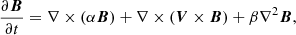
The dynamo converts kinetic energy of random (turbulent) flows into magnetic energy. The mean helicity of the random flow, that emerges because of the overall rotation and stratification, leads to the generation of magnetic fields at scales much larger than the correlation scale of the random flow (this is described as the α-effect). Differential rotation can accelerate the energy conversion by stretching the large-scale magnetic fields in the direction of the flow (the ω-effect). The spatial scale and structure of the magnetic field are controlled by the mean-field transport coefficients, quantifying the averaged induction effects of the random flows, and the large-scale velocity shear rate. The magnetic field structure also depends upon the geometric shape of the dynamo region (e.g. spherical, toroidal or flat). When the magnetic field is weak, so that its effect on the velocity field is negligible, the dynamo leads to an exponential amplification of the large-scale magnetic field. As the Lorentz force becomes stronger, the field growth slows down and the system gradually settles into a (statistically) steady state: the dynamo action saturates.
The mean-field dynamo equation has the form
 (1)
(1)
where B is the large-scale magnetic field, α and β are the turbulent transport coefficients representing the mean induction effects of the helical interstellar turbulence (the α-effect) and turbulent magnetic diffusion, respectively, and V is the large-scale velocity field. The latter is dominated by differential rotation but can also include galactic outflows (fountain or wind) and accretion.
Detailed reviews of the galactic dynamo and comprehensive references can be found in Ruzmaikin et al. (1988), Beck et al. (1996), Shukurov et al. (2007), and Shukurov & Subramanian (2018). We present here a very short overview of the theory with the number of specific references reduced to a minimum.
The mean-field galactic dynamo equation has been solved under various approximations that cover a wide range of galactic environments. Our goal is to present a general class of physically-motivated magnetic field models that can be used to fit observations without the need to delve too deeply into the theory. Thus, we present a parametrised model with the large-scale magnetic field in the form of an expansion over appropriate basis functions, specifically the modes of free decay which solve the diffusion equation in the disc and spherical geometries. The form of the magnetic structures obtained is controlled by the choice of the expansion coefficients. The large-scale magnetic field in the model consists of a superposition of approximate solutions of the kinematic mean-field dynamo equations for a thin disc (Sect. 3) and a spherical gaseous halo (Sect. 4). Our use of the dynamo equations is less restrictive than it might seem since their solutions can be used as a functional basis to represent a wide class of complex magnetic configurations, not necessarily produced by dynamo action, in terms of a small number of the expansion coefficients. Unlike representations in terms of the Euler potentials (Ferrière & Terral 2014), magnetic configurations presented here can be helical. Another advantage of our approach is that all variables and parameters of the model are either directly observable or related to observable quantities.
The approximate nature of the solutions that we use is due to the approximations adopted to solve the equations as well as the simple superposition of separate disc and halo solutions of the dynamo equation. Such a superposition is not quite consistent with the presumably non-linear nature of galactic dynamos. However, the non-linear effects do not, plausibly, affect the spatial distribution of the large-scale magnetic field too strongly and the marginally stable dynamo eigenfunctions often provide a satisfactory approximation for the non-linear solutions (Chamandy et al. 2014).
The analytic solutions of the mean-field dynamo equations for the galactic discs and halos presented here are obtained assuming that the disc is thin and the halo is spherical. The thin-disc solutions are applicable at those distances to the galactic centre s where h/s ≲ 0.1, where h is the scale height of the warm ionised gas that is assumed to host the mean magnetic field.
2.1. Symmetries of galactic magnetic fields
It is convenient to introduce cylindrical polar coordinates (s, ϕ, z) with the origin at the galactic centre and the z-axis parallel to the angular velocity Ω. Hence, Ω = (0, 0, Ω) and z = 0 at the galactic mid-plane. However, spherical coordinates (r, θ, ϕ) are natural for the halo, with the polar axis θ = 0 aligned with the z-axis of the cylindrical frame and the mid-plane (equator) at θ = π/2.
Solutions of the dynamo equation are sensitive to the geometry of the dynamo region. In a thin disc, large-scale magnetic fields of even parity strongly dominate, that is, Bs, ϕ(−z) = Bs, ϕ(z) and Bz(−z) = −Bz(z); this configuration corresponds to quadrupolar symmetry. Without dynamo action, quadrupolar magnetic fields in a thin disc decay slower than dipolar ones. As a result, for realistic values of parameters, dipolar magnetic fields can be supported by the dynamo only in the central parts of the discs of spiral galaxies, ≲1 kpc. In a quasi-spherical halo, however, both odd (dipolar) and even (quadrupolar) magnetic fields can be maintained with almost equal ease, with Br, ϕ(−z)= −Br, ϕ(z) and Bθ(−z) = Bθ(z) for the dipolar symmetry and Br, ϕ(−z) = Br, ϕ(z) and Bθ(−z) = −Bθ(z) in the quadrupolar field (with z = rcosθ). Moreover, magnetic fields in the two halves of the halo, z > 0 and z < 0, can be disconnected by the disc, so that the symmetry of the magnetic field in the halo is only weakly constrained. The model proposed here provides freedom in selecting any symmetry of the magnetic field in the disc and the halo independently.
Despite deviations from axial symmetry, mainly associated with the spiral pattern, galactic discs are sufficiently symmetric in azimuth that the axially-symmetric modes dominate the dynamo. Therefore, deviations from axial symmetry in the large-scale magnetic field, however strong they might be, can be included as distortions of a background axially symmetric magnetic structure. In this paper, we mainly consider axially symmetric galaxies and axially symmetric magnetic fields and discuss extensions to more general configurations in Sect. 5.3.
2.2. Boundary conditions
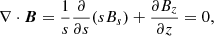
The simplest and best explored solutions of the mean-field dynamo equations are obtained with the so-called vacuum boundary conditions, that is, under the assumption that the electric current density outside the dynamo region is negligible in comparison with any electric currents within it. Equivalently, the magnetic diffusivity (inversely proportional to electric conductivity) outside the dynamo region is assumed to be much larger than within it. With vanishing electric current density, ∇ × B = 0, the magnetic field is potential.
Neglecting external electric currents in the gaseous halo appears to be reasonable given the low density of intergalactic plasma. Regarding galactic discs surrounded by a gaseous halo, it is important to note that the magnetic diffusivity relevant to a large-scale magnetic field is the turbulent diffusivity. Poezd et al. (1993) argue that the turbulent magnetic diffusivity in galactic haloes is about 50 times larger than in the disc. This justifies the application of vacuum boundary conditions to the large-scale magnetic field at the disc surface as well. In other words, we assume that the extension of the disc’s magnetic field into the halo is a potential magnetic field that adds to the magnetic field produced in situ in the halo.
In a thin disc, the vacuum boundary conditions have the form Bϕ(±h) = 0 and Bs(±h)≈0, where z = ±h(s) is the disc surface. The boundary condition for Bϕ is exact whereas the accuracy of the boundary condition for Bs is higher when the disc is thinner (Priklonsky et al. 2000; Willis et al. 2004). The potential magnetic field around the disc, that satisfies these boundary conditions, is purely vertical. The vacuum boundary conditions for the halo are Bϕ(rh) = 0 and ∇ × B = 0 at r > rh, where rh is the halo radius.
3. Magnetic field in the disc
3.1. Rotation curve and disc thickness
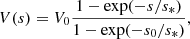
While the model can be applied to any galaxy, our choice of fiducial parameters is motivated by the Milky Way, with the disc rotation curve of Clemens (1985). To illustrate the impact of the rotation curve on the magnetic field, we also consider a flat rotation curve (i.e., the rotational speed is nearly independent of s at large distances from the disc axis),
 (2)
(2)
where s0 is a reference galactocentric distance defined below, V0 is the rotation speed at s = s0 and we take s* = 250 pc. The two rotation curves and the corresponding velocity shear rates, S = sdΩ/ds, are shown in Fig. 1.
 |
Fig. 1. Two choices for the rotation curve discussed in the text (upper panel) and the corresponding velocity shear rate S = sdΩ/ds (lower panel): the Milky Way rotation curve obtained from CO observations by Clemens (1985; solid) and a simpler rotation curve given by Eq. (2) (dashed). |
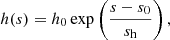
The disc scale height is assumed to increase exponentially with the cylindrical radius (a flared disc),
 (3)
(3)
where we adopt a flaring length scale of sh = 5 kpc, similar to that of the MW H I disc, and s0 is the Galactocentric distance of the Sun (Kalberla & Kerp 2009). In our fiducial model, we adopted the characteristic height h0 = 0.5 kpc, which is the scale height of the Lockman layer (Lockman 1984; Dickey & Lockman 1990) near the Sun.
The radius of the dynamo-active part of the disc is chosen to be sd = 17 kpc, similar to the radius of the supernova distribution in the MW (Case & Bhattacharya 1998). The fiducial values of the parameters that appear in the model (which are also input parameters for the GALMAG code) are shown in Table 1. Parameters of the halo are introduced in Sect. 4.2.
Fiducial parameter values and input parameters of the GALMAG code.
3.2. Thin-disc dynamos
In terms of cylindrical coordinates (s, ϕ, z), the radial and azimuthal components of the axisymmetric α2ω-dynamo Eq. (1) can be written as
![Mathematical equation: $$ \begin{aligned} \frac{\partial B_s}{\partial t}&= - \frac{\partial (\alpha B_\phi )}{\partial z} + {\beta } \frac{\partial ^2 B_s}{\partial z^2} + {\beta } \frac{\partial }{\partial {s}}\left[ \frac{1}{{s}}\frac{\partial ({s} B_s)}{\partial {s}} \right], \end{aligned} $$](/articles/aa/full_html/2019/03/aa34642-18/aa34642-18-eq4.gif) (4)
(4)
![Mathematical equation: $$ \begin{aligned} \frac{\partial B_\phi }{\partial t}&= S B_s + \frac{\partial (\alpha B_s)}{\partial z} + {\beta } \frac{\partial ^2 B_\phi }{\partial z^2} + {\beta } \frac{\partial }{\partial {s}}\left[ \frac{1}{{s}}\frac{\partial ({s} B_\phi )}{\partial {s}} \right], \end{aligned} $$](/articles/aa/full_html/2019/03/aa34642-18/aa34642-18-eq5.gif) (5)
(5)
where S = s ∂Ω/∂s is the velocity shear due to differential rotation. We do not exhibit the equation for Bz since, in a thin disc, it decouples from the equations shown and can be solved separately (equivalently, Bz can be derived from ∇ ⋅ B = 0).
It is convenient to use dimensionless variables, denoted with tilde,
 (6)
(6)
where s0 is the reference cylindrical radius within the disc – for example, s0 = s⊙ ≈ 8.5 kpc is a convenient choice in the MW. Using different length units across and along the disc allows us to make the disc thinness explicit and quantified with the (small) aspect ratio
 (7)
(7)
The large-scale velocity is measured in the units of a characteristic rotational speed V0 = V(s0),
 (8)
(8)
Velocity shear due to differential rotation is non-dimensionalised similarly,
 (9)
(9)
The unit of time is the turbulent magnetic diffusion time across the disc. With βd the turbulent magnetic diffusivity in the disc, the dimensionless time is
 (10)
(10)
The magnitude of the α-effect can be estimated as
 (11)
(11)
where l and v are the turbulent scale and speed, and the corresponding fiducial value is used to non-dimensionalise α:
 (12)
(12)
The magnitude of α cannot exceed α = v because it is a measure of the helical part of the turbulent flow speed, hence α/v cannot exceed unity. This limit is usually important only in the central parts of galaxies (where the thin-disc approximation does not apply anyway). Equation (11) gives the magnitude of α and its dependence on s through the variations of Ω and h with s. It is expected that α is an odd function of z. Gressel et al. (2008a,b) and Bendre et al. (2015) confirm this and discuss the dependence of α on z in numerical simulations of the supernova-driven interstellar medium. We adopt a factorised form for α(s, z),
 (13)
(13)
where we assume that l, in Eqs. (11) and (12), is independent of s. The model can be generalised straightforwardly to more general forms of α(s, z).
When galactic outflow is neglected, the dynamo is fully characterised by two dimensionless control parameters that quantify the intensity of the mean magnetic induction due to helical turbulence and differential rotation, respectively:
 (14)
(14)
where the subscript “d” refers to the disc (similar parameters are defined slightly differently in the halo – see Sect. 4).
In terms of dimensionless variables, Eqs. (4) and (5) reduce to
![Mathematical equation: $$ \begin{aligned} \frac{\partial B_s}{\partial \widetilde{t}}&= -{R_{\alpha \text{ d}}} \frac{\partial (\widetilde{\alpha }B_\phi )}{\partial \widetilde{z}} + \frac{\partial ^2 B_s}{\partial \widetilde{z}^2} + \epsilon ^2 \frac{\partial }{\partial \widetilde{{s}}} \left[ \frac{1}{\widetilde{{s}}}\frac{\partial (\widetilde{s} B_s)}{\partial \widetilde{{s}}} \right], \end{aligned} $$](/articles/aa/full_html/2019/03/aa34642-18/aa34642-18-eq15.gif) (15)
(15)
![Mathematical equation: $$ \begin{aligned} \frac{\partial B_\phi }{\partial \widetilde{t}}&= {R_{\omega \text{ d}}} \widetilde{S} B_s + {R_{\alpha \text{ d}}} \frac{\partial (\widetilde{\alpha } B_s)}{\partial \widetilde{z}} + \frac{\partial ^2 B_\phi }{\partial \widetilde{z}^2} + \epsilon ^2 \frac{\partial }{\partial \widetilde{{s}}} \left[\frac{1}{\widetilde{{s}}}\frac{\partial (\widetilde{{s}}B_\phi )}{\partial \widetilde{{s}}} \right]\cdot \end{aligned} $$](/articles/aa/full_html/2019/03/aa34642-18/aa34642-18-eq16.gif) (16)
(16)
It is now clear that the solutions are fully determined by Rαd, Rωd,  ,
,  and ϵ.
In a thin disc, the magnetic field distribution along z is established over a time scale h2/βd ≃ 5 × 10⁸ yr which is ϵ−2 = (s0/h0)2 times shorter than the time scale at which the radial distribution evolves,  . Because of this difference, the radial derivatives in Eqs. (15) and (16) have ϵ2 as a factor. Therefore, the magnetic field distribution in a thin disc can be represented as a local solution (at a given galactocentric distance s), b(z; s), modulated by an envelope Q(s). The local solution also depends on s since α, S and h vary with s, but this variation is parametric. It is convenient to normalise the local solution to unit surface magnetic energy density,
  , at all values of s: then Q(s) represents magnetic field strength at the galactocentric radius s (an envelope of the local solutions). Thus, asymptotic solutions of Eqs. (15) and (16) for ϵ ≪ 1 have the form
 (17)
(17)
The magnetic field varies exponentially with time at a rate Γ in the kinematic dynamo stage. In a saturated thin-disc dynamo, the solution has a similar form but with Γ = 0 (Poezd et al. 1993). The local solution is discussed in Sect. 3.3, whereas Sect. 3.4 presents the radial solution Q(s).
To simplify the notation, we use exclusively the dimensionless variables with the tilde suppressed in the remaining part of this section unless otherwise stated.
3.3. Local solutions
Governing equations for the local solution, b = exp(γt) (bs, bz), follow from Eqs. (15) and (16) when we put ϵ = 0:
![Mathematical equation: $$ \begin{aligned} \gamma ({s}) b_s&=-{R_{\alpha \text{ d}}}\frac{\partial }{\partial z}\left[\alpha ({s},z) b_\phi \right]+\frac{\partial ^2 b_s}{\partial z^2}, \end{aligned} $$](/articles/aa/full_html/2019/03/aa34642-18/aa34642-18-eq22.gif) (18)
(18)
![Mathematical equation: $$ \begin{aligned} \gamma ({s}) b_\phi&= {R_{\omega \text{ d}}} S({s}) b_s +\frac{\partial ^2 b_\phi }{\partial z^2}+ {R_{\alpha \text{ d}}} \frac{\partial }{\partial z}\left[\alpha ({s},z) b_s\right]. \end{aligned} $$](/articles/aa/full_html/2019/03/aa34642-18/aa34642-18-eq23.gif) (19)
(19)
To allow for the disc flaring, we introduce the following new variables:
 (20)
(20)
Since Rαd ≪ Rωd at s ≳ 1 kpc in most spiral galaxies, we can omit the term proportional to Rαd in Eq. (19), thus obtaining the αω-dynamo approximation:
![Mathematical equation: $$ \begin{aligned} \widehat{\gamma }({s})\widehat{b}_s&=-\frac{\partial }{\partial {\widehat{z}}}\left[ a(z) b_\phi \right] +\frac{\partial ^2 \widehat{b}_s}{\partial {\widehat{z}}^2}, \end{aligned} $$](/articles/aa/full_html/2019/03/aa34642-18/aa34642-18-eq25.gif) (21)
(21)
 (22)
(22)
where a(z), the z-dependent part of α(s, z), is defined in Eq. (13) and 𝒟(s), the local dynamo number, includes the radial variation of the dynamo parameters:
 (23)
(23)
It is also convenient to introduce the local (in galactocentric radius) values of Rαd and Rωd,
 (24)
(24)
so that 𝒟 = ℛαℛω. The normalisation condition for the local solution reduces to
 (25)
(25)
where we have neglected  because this component of magnetic field is, on average, weaker than the other two. To this order in ϵ, bz does not enter the equations for bs and bϕ and can be solved for separately. The result can be shown to be identical to that obtained from ∇ ⋅ B = 0.
The vacuum boundary conditions are
 (26)
(26)
Since a(z) is an odd function of z, solutions of Eqs. (21) and (22) split into two independent classes, even and odd in z (or quadrupolar and dipolar, respectively). These can be distinguished using the symmetry conditions at the galactic mid-plane,
 (27)
(27)
 (28)
(28)
Approximate solutions for both parity families can be obtained in the form of an expansion over the free-decay modes obtained as solutions of Eqs. (21) and (22) for a(z) = 𝒟(s)=0. The procedure is discussed in detail by Shukurov et al. (2008) and Chamandy et al. (2014), and here we only provide the results.
From Eqs. (21)–(27), we obtain the following approximate solutions of quadrupolar symmetry, for  :
:
![Mathematical equation: $$ \begin{aligned} b_s(z;{s})&\approx \mathcal{R} _\alpha {({s})} K_0({s}) \left[\cos \frac{\pi z}{2h({s})} +\frac{3\sqrt{-{\mathcal{D} }({s})}}{4\pi ^{3/2}} \cos \frac{3\pi z}{2h({s})}\right] ,\end{aligned} $$](/articles/aa/full_html/2019/03/aa34642-18/aa34642-18-eq35.gif) (29)
(29)
 (30)
(30)
![Mathematical equation: $$ \begin{aligned} \gamma ({s})&\approx \frac{1}{h^2({s})}\left[ -\frac{\pi ^2}{4}+\frac{1}{2}\sqrt{-\pi {\mathcal{D} }({s})} \right] , \end{aligned} $$](/articles/aa/full_html/2019/03/aa34642-18/aa34642-18-eq37.gif) (31)
(31)
where
![Mathematical equation: $$ \begin{aligned} K_0{({s})} = \left[1 - \frac{4 {\mathcal{D} }(s)}{\pi } - \frac{9 {\mathcal{D} }(s)}{16 \pi ^{3}}\right]^{-1/2} \end{aligned} $$](/articles/aa/full_html/2019/03/aa34642-18/aa34642-18-eq38.gif) (32)
(32)
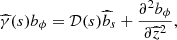
is the normalization factor obtained using Eq. (25). These solutions are shown in Fig. 2. Equation (31) provides the critical value of the local dynamo number required for the local amplification and maintenance of the magnetic field: γ ≥ 0 for 𝒟 ≤ 𝒟c ≈ −π3/4 ≈ −8. Other choices of the functional form of  lead to slightly different values of the critical dynamo number (e.g. −11 for a = z), but the difference hardly has any practical consequences.
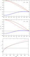 |
Fig. 2. Comparison of the local quadrupolar eigenfunctions for 𝒟 = −20 (upper panel) and −50 (middle panel) obtained from numerical solution of the local Eqs. (21) and (22) with the approximate eigenfunctions Eqs. (29) and (30): bϕ from the numerical solution are shown solid (red) and bs, dashed (blue); their approximate counterparts are shown with dotted curves of the matching colour. The eigenfunctions are normalised to bϕ(0) = 1. Bottom panel: numerical (black, solid) and approximate, Eqs. (31) (red, dashed), solutions for the local growth rate as a function of the local dynamo number. |
In the odd-parity solutions, the term proportional to (−𝒟)1/2 in bs vanishes for  . Therefore, it is more convenient to use a similar solution with
  that satisfies the symmetry condition Eq. (28), here written to the lowest order in (−𝒟)1/2:
 (33)
(33)
 (34)
(34)
 (35)
(35)
with
![Mathematical equation: $$ \begin{aligned} K_1{({s})} = \left[1 - 4 {\mathcal{D} }(s)\right]^{-1/2}\,. \end{aligned} $$](/articles/aa/full_html/2019/03/aa34642-18/aa34642-18-eq45.gif) (36)
(36)
The dipolar modes can be excited, γ ≥ 0, for 𝒟 ≤ −2π4 ≈ −195, a threshold much higher than for the quadrupolar modes. This is true for any plausible form of  and explains the predominance of quadrupolar magnetic fields in thin discs.
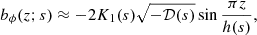
The local solutions are derived, formally, for |𝒟|≪1 but they remain reasonably accurate for |𝒟| as large as about 50 or more (Ji et al. 2014). We compare in Fig. 2 the local quadrupolar eigenfunctions obtained from numerical solution of Eqs. (21) and (22) with the approximate solutions Eqs. (29)–(31) for 𝒟 = −20 and −50, values typical of the main parts of spiral galaxies (see Fig. 3).
 |
Fig. 3. Radial profiles of the local dynamo number (upper panel) and the local growth rate of the quadrupolar solutions (lower panel) for the flat rotation curve Eq. (2) (solid) and for the MW rotation curve of Clemens (1985; dashed). Upper panel: critical dynamo number 𝒟c ≈ −π3/4 is shown dotted for reference. |
The local eigenfunctions presented above are approximate solutions of the mean-field dynamo equations. However, the functional basis of these solutions, the free-decay modes, can be used as a complete functional basis to represent any magnetic field configuration. The free-decay modes are solutions of Eqs. (21) and (22) with a(z) = 0 and 𝒟(s) = 0, so that the equations decouple and can easily be solved. Normalised as in Eq. (25), the dipolar and quadrupolar free-decay eigenfunctions and eigenvalues (identified with superscripts d and q, respectively) have the following respective forms with n = 1, 2, 3, …:
 (37)
(37)
![Mathematical equation: $$ {\boldsymbol{b}}_n^{({\rm{q}})} = \left( {\begin{array}{*{20}{c}} {\cos \left[ {\pi \left( {n - {\textstyle{1 \over 2}}} \right)\hat z} \right]}\\ 0 \end{array}} \right),\quad {\boldsymbol{b}}_n^{({\rm{q}})\prime } = \left( {\begin{array}{*{20}{c}} 0\\ {\cos \left[ {\pi \left( {n - {\textstyle{1 \over 2}}} \right)\hat z} \right]} \end{array}} \right), $$](/articles/aa/full_html/2019/03/aa34642-18/aa34642-18-eq48.gif) (38)
(38)
 (39)
(39)
The free-decay disc modes are double degenerate as two orthogonal modes of the same parity (distinguished by prime) correspond to each eigenvalue.
3.4. Radial solution
When Eq. (17) is substituted into Eqs. (15) and (16), and Eqs. (18) and (19) are allowed for, equations for both Bs and Bϕ reduce to the same equation for Q(s), that is,
![Mathematical equation: $$ \begin{aligned} \epsilon ^2\frac{\partial }{\partial {s}}\left[ \frac{1}{{s}}\frac{\partial }{\partial {s}}({s} Q)\right] +[\gamma (s)-\Gamma ]Q = 0, \end{aligned} $$](/articles/aa/full_html/2019/03/aa34642-18/aa34642-18-eq50.gif) (40)
(40)
where γ(s) is the local growth rate obtained as a part of the local solution, Eq. (31) or (35). This equation applies to both even and odd local solutions, and to both α2ω and αω-dynamos, that is, with and without the term proportional to Rαd in Eq. (19). The boundary conditions adopted are
 (41)
(41)
The condition at s = 0 follows from axial symmetry, whereas that at the outer boundary of the dynamo-active region s = sd is adopted for the sake of simplicity.
When Ω(s) and h(s) are known, the global growth rate Γ and the radial distribution of the magnetic field strength Q(s) can be obtained by solving Eq. (40) numerically. However, for our present purposes it is more useful to obtain an approximate analytical solution for Q(s). This allows faster computations at the cost of an additional approximation. When the magnetic field model is used in Bayesian analyses, the computation speed is of primary importance.
To obtain a simple analytical solution of Eq. (40), consider γ to be a constant, γ = γ0, within the disc radius, s < sd, and zero outside,
 (42)
(42)
A suitably averaged value of γ(s) within the disc can be adopted for γ0. The relevance of this approximation depends on the specific case, particularly the rotation curve and the rate of the disc flaring, as shown in Fig. 3. The inner parts of the disc, s ≲ 1 kpc, should be disregarded since the thin-disc approximation is not applicable there. At s ≳ 1 kpc, the approximation γ(s) = const does not appear unreasonable, especially for the Milky Way rotation curve, as shown in the lower panel of Fig. 3.
For γ(s) of Eq. (42), Eq. (40) with boundary conditions Eq. (41) can be solved to yield the eigensolutions
 (43)
(43)
 (44)
(44)
where J1(x) is the standard Bessel function (of order one) and kn ≈ 3.83, 7.02, 10.17, … are its zeros, thus, J1(kn) = 0. The first four modes of Qn(s) are shown in Fig. 4. Independently of the form of γ(s), the lowest radial mode, Q1(s), is sign-constant but Qn(s) has n − 1 zeros, and thus the scale of variation of Qn(s) decreases with n. This feature of the solution is responsible for the reversals of the large-scale magnetic field discussed in Sect. 3.9.
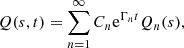
The evolving radial distribution of magnetic field is obtained as a superposition of the eigensolutions of Eq. (40):
 (45)
(45)
where, in the context of dynamo models, the coefficients Cn are determined by the initial conditions. Alternatively, the eigenfunctions Qn(s)b(z; s) can be used as the basis functions to represent a given magnetic field with exp(Γnt) absorbed into Cn. The set of radial eigenfunctions Qn is complete, so that any radial distribution of magnetic field can be represented in this form. The only constraint on the form of the solution is due to the fact that the set of the local solutions b is incomplete. Nevertheless, a wide class of magnetic field distributions along z can be represented as a superposition of various quadrupolar and dipolar local modes, so that the lack of the functional completeness of the local solutions is not likely to be restrictive in practice. Otherwise, the complete set of local free-decay modes  of Eqs. (37)–(39) can be used instead of the local dynamo solutions to construct a more general expansion over a complete set of basis functions of the form
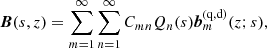
which can be used to parametrise (in terms of the coefficients Cmn) an arbitrary magnetic field that does not need to be a solution of the dynamo equations.
3.5. Vertical magnetic field
The axially symmetric vertical component of the magnetic field, Bz, can be obtained from
 (46)
(46)
using Bs(s, z) = bs(z; s)Q(s) from Eq. (29) or (33), and Eq. (43). We have assumed that γ0 = const to derive the simple form Eq. (43), implying 𝒟 = const. It is therefore justifiable to neglect the dependence of 𝒟, Ω and h on s when differentiating Bs in Eq. (46) and only retain the dependence of Q on s (this simplification can easily be relaxed if required). By virtue of linearity, Eq. (46) can be solved for each radial mode n separately:
![Mathematical equation: $$ \begin{aligned} -\frac{\partial B_z^{(n)}}{\partial z}&=\frac{1}{{s}}\frac{\partial }{\partial {s}}({s} B_s^{(n)})= \mathcal{R} _\alpha K_0 C_n\frac{1}{{s}} \frac{\mathrm{d} }{\mathrm{d} {s}}\left[{s} J_1(k_n{s}/{s}_\text{ d})\right]\nonumber \\&\quad \times \left(\cos \frac{\pi z}{2h({s})}+ \frac{3}{4\pi ^{3/2}}\sqrt{-{\mathcal{D} }({s})} \cos \frac{3\pi z}{2h({s})}\right)\cdot \end{aligned} $$](/articles/aa/full_html/2019/03/aa34642-18/aa34642-18-eq59.gif) (47)
(47)
Then, for the quadrupolar parity,
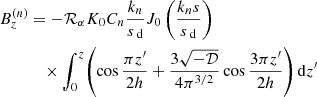 (48)
(48)
where the dependence of ℛα 𝒟, h and K0 on s should be allowed for.
3.6. Magnetic field in the disc
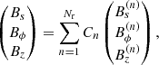
We can now collect the solutions from Sects. 3.3–3.5 to write the approximate solution of the dynamo equation (evolving or at a fixed time) for a thin disc as a sum of Nr radial eigenmodes,
 (49)
(49)
where, for the quadrupolar symmetry,
![Mathematical equation: $$ \begin{aligned} B_s^{(n)}&= K_0({s}) \mathcal{R} _\alpha ({s}) J_1(k_n {s}/{s}_\text{ d}) \nonumber \\&\quad \times \left[ \cos \frac{\pi z}{2 h({s})} +\frac{3\sqrt{-{\mathcal{D} }({s})}}{4\pi ^{3/2}} \cos \frac{3\pi z}{2h({s})}\right],\end{aligned} $$](/articles/aa/full_html/2019/03/aa34642-18/aa34642-18-eq62.gif) (50)
(50)
 (51)
(51)
![Mathematical equation: $$ \begin{aligned} B_z^{(n)}&= -\frac{2k_n h({s})}{\pi {s}_\text{ d}} K_0({s}) \mathcal{R} _\alpha ({s}) J_0(k_n{s}/{s}_\text{ d}) \nonumber \\&\quad \times \left[\sin \frac{\pi z}{2h({s})} +\frac{\sqrt{-{\mathcal{D} }({s})}}{4\pi ^{3/2}} \sin \frac{3\pi z}{2h({s})}\right], \end{aligned} $$](/articles/aa/full_html/2019/03/aa34642-18/aa34642-18-eq64.gif) (52)
(52)
and similarly for the dipolar symmetry. The local dynamo parameters 𝒟(s) and ℛα(s) are defined in Eqs. (23) and (24), whereas an example of the form of h(s) is given by Eq. (3). In what follows (and in the GALMAG code), we normalise each eigenmode so that each expansion coefficient represents the strength of the corresponding part of the magnetic field at the reference radius s0, that is, |Cn|=|B(n)(s0, 0)|.
The coefficients Cn can be chosen to fix the strength and to reproduce any radial distribution of the magnetic field. For instance, when used to approximate the magnetic field observed in the disc, Cn are used to fit the observations to a desired accuracy. When used to simulate a growing magnetic field, its evolution is introduced through  , where the initial values
  at t = 0 are obtained from the similar expansion for the seed magnetic field. Galactic evolution can be included by an appropriate time variation of 𝒟(s), Ω(s), h(s) and sd.
3.7. Dynamo parameters
In order to use the solution presented above, the dimensionless dynamo control parameters Rαd and Rωd have to be specified. We adopt the reference radius s0 = s⊙ ≈ 8.5 kpc and, correspondingly, V0 = 220 km s−1 and S0 = −35 km s−1 kpc−1 as obtained from the rotation curve. An estimate of the turbulent magnetic diffusivity widely used in various applications derives from the mixing length theory,
 (53)
(53)
where l and v are the turbulent scale and speed, respectively. With l ≃ 50 pc (see Hollins et al. 2017, and references therein) and v ≃ 10 km s−1 (e.g. Mac Low & Klessen 2004), we have β ≃ 5 × 1025 cm2 s−1. Equations (53) and (14) then yield
 (54)
(54)
A summary of parameters used by GALMAG and their fiducial values can be found in Table 1.
3.8. The role of the disc flaring and details of the rotation curve
Figure 5 shows the vertical cross section of magnetic field in the disc, constructed using the first two radial eigenmodes with (C1, C2) = (4.6 μG, −1.5 μG). These distributions have an absolute maximum of |B| at large s. This happens because the local dynamo number of Eq. (23) increases with galactocentric distance in an exponentially flared disc, 𝒟 ∝ ΩSh2 ∝ s−2 exp(2s/sh) for a flat rotation curve, Ω ∝ S ∝ s−1. If h indeed increases with s faster than s2, the outer parts of galactic discs can have relatively strong magnetic fields at early stages of magnetic field growth when these kinematic solutions apply. Such distributions may occur in young and evolving galaxies. Non-linear dynamo effects eventually limit the local magnetic field strength to a value related to equipartition between magnetic and turbulent kinetic energies, B2 ≈ 4πρv2(𝒟/𝒟cr − 1)∝s−2 exp(2s/sh − s/sρ) assuming that ρ ∝ exp(−s/sρ). The radial profile of magnetic field strength then depends on the relation between the radial length scales of the gas density and disc thickness. The number density of H I in the MW has sρ ≃ 3 kpc (Kalberla & Kerp 2009) which is close to sh/2 ≃ 2.5 kpc. Therefore, we cannot exclude the possibility that the magnetic field remains strong in the outer MW. The effective boundary of the dynamo active region is then determined by the rapid increase of the local dynamo time scale γ−1(s)≃h2(s)/βd with s in a flared disc: this time scale exceeds 1010 yr where h ≳ 1 kpc for βd = 5 × 1025 cm2 s−1, and the growth of magnetic field becomes practically negligible. For h(s) given by Eq. (3), this happens at s ≳ 11 kpc provided βd is independent of s. When the magnetic field is stronger in the outer parts of the disc, the boundary condition Q(sd) = 0 may be too restrictive. We have considered solutions with ∂(sQ)/∂s|s = sd = 0 to confirm that the magnetic field distribution in the main part of the disc is not significantly affected but the outer field maximum becomes more pronounced.
The increase of the local dynamo number with distance from the galactic centre enhances the large-scale magnetic field in the outer parts of a galactic disc in either the kinematic or saturated dynamo. As a result, the magnetic field energy density may decrease with radius slower than other energy densities in the interstellar medium, as suggested by Beck (2007).
3.9. Field reversals along the galactocentric radius
Magnetic field reversals can be reproduced naturally in the model because the radial eigenfunction Qn(s) has n − 1 zeros. With an appropriate selection of the expansion coefficients Cn, any desired number of reversals located at any prescribed positions can be produced. While the strength of the magnetic field is controlled by the magnitudes of the expansion coefficients Cn, the number of reversals and their positions along the radius are controlled by the ratios of the coefficients, for instance, Cn/C1. Since Q2(s) has one zero while Q3(s) has two zeros, retaining only the two leading terms in the expansion Eq. (49) allows us to obtain a magnetic field with one radial reversal, whereas in order to have two reversals, Q3(s) needs to be included. To help selecting the coefficients as required to obtain a magnetic field that has a given number of reversals at desired positions, we present Fig. 6 where the ranges of C2/C1 and C3/C1 that produce one or two reversals can be read off the left-hand panel. The desired positions of the reversals can be converted into the coefficient ratios using the middle and right-hand panels. Similar diagrams can be constructed for any number of reversals if required.
 |
Fig. 6. Number and positions of magnetic field reversals along the disc radius, for a magnetic field constructed by a superposition of the first three fastest growing eigenfunctions, Qn(s) with n = 1, 2, 3, for the fiducial choice of parameters shown in Table 1. Left-hand panel: number of the field reversals (colour coded as indicated with the colour bar on the right of the panel) for various ratios of the expansion coefficients Cn/C1. Middle and right-hand panels: galactocentric distances of the inner and outer reversal, srev,1 and srev,2 respectively, colour coded with the colour bar to the right of each panel. White colour indicates the absence of the corresponding reversal. |
Figure 7 illustrates the structure of axisymmetric magnetic fields that have radial reversals. Model A, with a reversal at s = 7 kpc, represents the same field as in the bottom right panel of Fig. 5. Model B, constructed using the three leading eigenfunctions, has reversals at s = 7 and 12 kpc. In both models, the magnetic field is normalised so that the azimuthal magnetic field, shown in Fig. 7c, has the strength 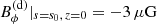 in the mid-plane z = 0 at the reference radius s = s0 = 8.5 kpc.
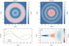 |
Fig. 7. Two examples of the disc magnetic field with radial reversals. Top panels: field strength in the galactic mid-plane is shown colour coded with arrows showing the direction and strength of the magnetic field projected onto the mid-plane. Model A, shown in (panel a), has a reversal at s = 7 kpc and corresponds to the same field as in the bottom right panel of Fig. 5. Model B, shown in (panel b), has the same parameters except for having two reversals at s = 7 and 12 kpc. Panel c: azimuthal magnetic field in the two models. Panel d: vertical cross-section of Model B is shown, with the magnitude of azimuthal magnetic field indicated with colour and arrows showing the projection of the magnetic field onto the (xz)-plane. |
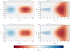 |
Fig. 5. Sensitivity of the magnetic field structure to the rotation curve and disc flaring, illustrated with magnetic fields constructed using fiducial parameters and (C1, C2) = (4.6 μG, −1.6 μG). The strength of the azimuthal component of the magnetic field is colour coded, while arrows indicate the direction and strength of the poloidal magnetic field. Details of the disc models are indicated above each frame and the disc scale height is indicated with a dotted line on the left and a dashed line on the right. Strong differential rotation near the galactic centre leads to a strong magnetic field, especially in a flat disc. In a flared disc, which is thinner at small s, the field strength near the galactic centre is reduced but the outer region has a stronger field. |
Figure 7d shows the vertical cross-section (a meridional plane) of the magnetic structure in Model B to demonstrate that, in a thin disc, the horizontal magnetic field components dominate over the vertical field, |Bϕ| > |Bs|≫|Bz|, only on average. Locally, and especially near the reversals and the disc axis, the vertical magnetic field dominates. This is a direct consequence of the solenoidality of magnetic field: if Bϕ and Bs are weak, Bz needs to be stronger to ensure that ∇ ⋅ B = 0. The dominance of Bϕ over Bs is less general in origin: this is a consequence of the stretching of the radial magnetic field by differential rotation, and the larger is the velocity shear the larger is the ratio |Bϕ/Bs| and the smaller is the magnitude of the magnetic pitch angle p = arctan(Bs/Bϕ).
4. Magnetic field in the halo
Magnetic field in the spherical halo is obtained as the perturbation solution of the mean-field dynamo equation with free-decay eigenfunctions as the unperturbed solutions. This approach is similar to that employed to obtain the local disc solution in Sect. 3.3.
In the spherical halo, it is convenient to use spherical coordinates (r, θ, ϕ). As for the disc, we define convenient dimensionless variables distinguished by the tilde: spherical radius and time are measured in the units of the halo radius rh and the corresponding magnetic diffusion time, respectively,
 (55)
(55)
with βh the turbulent magnetic diffusivity in the halo. The velocity field and the α-coefficient are normalised as
 (56)
(56)
where αh is the α-coefficient at the north pole, (r, θ) = (rh, 0), and Vh is the equatorial rotation velocity at the boundary (r, θ) = (rh, π/2).
In terms of the dimensionless variables, the mean-field dynamo Eq. (1) reduces to
 (57)
(57)
where we defined, analogously to Eq. (14), the dynamo parameters
 (58)
(58)
To avoid excessively heavy notation, we suppress the tilde on the dimensionless variables and work exclusively with dimensionless variables unless otherwise stated.
Solutions of Eq. (57), growing or decaying at a rate Γ, are sought in the form of an expansion
 (59)
(59)
in the free-decay modes Bi which are obtained as solutions of Eq. (57) with Rαh = Rωh = 0,
 (60)
(60)
where γi < 0 is the rate of exponential decay of the mode Bi. Outside the halo, an electromagnetic vacuum is assumed, implying a potential magnetic field, ∇ × Bi = 0. The boundary conditions that ensure a continuous matching, at the halo boundary r = 1, of the interior magnetic field to a potential exterior magnetic field that decays at infinity as the point dipole (the lowest magnetic multipole) are given by (Moffatt 1978)
![Mathematical equation: $$ \begin{aligned} \left[{\boldsymbol{B}}_i\right]=0 \ \text{ at} \ r=1, \qquad {\boldsymbol{B}}_i=\mathcal{O} \left(r^{-3}\right) \ \text{ for} \ r\rightarrow \infty , \end{aligned} $$](/articles/aa/full_html/2019/03/aa34642-18/aa34642-18-eq76.gif) (61)
(61)
where the square brackets denote the jump of the corresponding quantity.
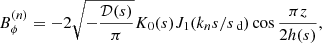
The spatial form and decay rates of the spherical modes of free decay are derived in Appendix A; here we briefly discuss their properties. The free decay modes form a complete, orthonormal set of basis functions (related to spherical harmonics), each either purely poloidal (comprising the field components Br and Bθ) or purely toroidal (consisting of Bϕ alone). They can be divided into two classes based on their symmetry about the equator θ = π/2: the symmetric modes are quadrupolar (indicated with superscript “q”) whereas the anti-symmetric modes have a dipolar symmetry (superscript “d”). Their analytic forms can be found in Appendices A.1 and A.2, respectively. Figure 8 shows the structure of the four free-decay modes of each symmetry that have the largest γi.
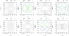 |
Fig. 8. Eight spherical free-decay eigenfunctions Bi of the smallest decay rates. Each mode is either purely toroidal or purely poloidal. Top row: modes symmetric with respect to the mid-plane z = 0 (quadrupolar modes), while the modes in the bottom row are anti-symmetric (dipolar). For the poloidal modes, arrows represent the projection of the magnetic field on the (xy)-plane. For the toroidal modes, contours show the strength of the azimuthal component of the magnetic field with the normalisation Eq. (A.20). The decay rate of each mode γ is shown at the top of each panel. |
4.1. The perturbation solution
Equation (57) can be conveniently written as
 (62)
(62)
where the perturbation operator  corresponding to the α2ω-dynamo is given by
 (63)
(63)
As discussed in Appendix B, GALMAG has also an option to use the αω-dynamo operator but this approximation may be questionable in the case of the halo.
We substitute Eq. (59) into Eq. (62), take the scalar product of the result with Bi and integrate over the whole space. As a result, we obtain a homogeneous system of algebraic equations for the expansion coefficients ai of the form
 (64)
(64)
where
 (65)
(65)
are the matrix elements of the perturbation operator, with integration performed over the whole space. Since the operator  transforms a poloidal field into a toroidal one and vice versa (and the two are orthogonal), it follows that Wii = 0 and each non-vanishing matrix element involves at least one toroidal and one poloidal free-decay eigenfunction. Because the toroidal eigenfunctions vanish at r > rh, the integrals are in fact restricted to the interior of the halo. The solvability condition of the system of equations for ai, the vanishing of its determinant, yields the growth rate Γ. Once the matrix elements have been computed and the system Eq. (64) has been solved for ai, Eq. (59) yields the solution of the dynamo equation. One of the coefficients ai remains arbitrary because the dynamo equation is linear in magnetic field and hence its solution is determined up to an arbitrary factor. This freedom is used to fix the magnetic field strength at any desired value.
4.2. Parameters of galactic haloes
Velocity fields in galactic haloes are poorly known. Random velocities are likely to increase with altitude, and H I observations of Kalberla et al. (1998; see also Kalberla & Kerp 2009) suggest a three-dimensional velocity dispersion of about 100 km s−1, close to the sound speed at a temperature 106 K. The scale of these motions is uncertain. The size of supernova remnants above the galactic disc is expected to be of order 0.3 kpc (McKee & Ostriker 1977). The size of the hot gas bubbles rising from the disc and the scale of the Parker instability are of order 0.5–1 kpc (e.g. Rodrigues et al. 2016). Adopting the random speed and scale as v = 100 km s−1 and l = 0.5 kpc, the turbulent diffusivity is estimated by  . The corresponding magnetic diffusion time across the halo radius is
  .
.
The knowledge of the variation of the rotation speed with position within galactic haloes is rather rudimentary. Both the rotational speed and its radial gradient decrease in spiral galaxies with distance from the mid-plane, with a typical vertical gradient of order ∂V/∂z = −(15–25) km s−1 kpc−1 within a few kiloparsecs from the mid-plane (Zschaechner et al. 2015). In our fiducial model, the halo is assumed to have a rotation curve of the form
 (66)(expressed in terms of dimensional variables), with
  the unit azimuthal vector and
 (67)
(67)
where the turnover radius is chosen to be sv = 3 kpc, the typical value found in observations and simulations of MW-type galaxies (Reyes et al. 2011; Schaller et al. 2015). For simplicity, the rotation curve of Eqs. (66) and (67) has no z-dependence but it can easily be introduced. The role of the variation of Ω with z is to produce Bϕ from Bz, arguably a process somewhat less important than the stretching of the radial magnetic field in the azimuthal direction at a rate S = s∂Ω/∂s.
We adopt a simple form for the α-coefficient often used in spherical mean-field dynamo models; in dimensional variables,
 (68)
(68)
implying the largest absolute value of α near the poles whilst α also vanishes at the equator, reflecting the fact that the mean helicity of the random flows is produced by the Coriolis force.
We consider an axially symmetric magnetic field in the halo and assume that the dynamo operates within a region of rh = 15 kpc in radius. We take Vh = 220 km s−1 (similar to that in the disc). With the turbulent magnetic diffusivity βh = 5 × 1027 cm2 s−1, this leads to Rωh ≃ 200.
Estimating Rαh in the halo is more difficult given the uncertainty of the random flow parameters. The standard estimate of Eq. (11) yields αh ≃ l2Ω/h ≃ 1 km s−1 and Rαh = αhrh/βh ≃ 1 for Ω = 26 km s−1 kpc−1 and h = 3 kpc, the gas density scale height in the halo. As the fiducial value for Rαh, we select its marginal value corresponding to the vanishing dynamo growth rate (see Sect. 4.3 for details): Rαh(q) = 4.3 for symmetric solutions and Rαh(d) = 8.1 for anti-symmetric ones. The symmetric mode is preferred to the anti-symmetric one only slightly, Rαh(q)/Rαh(d) ≃ 0.5 for the marginal values. The similarity of the marginal values of Rαh for the dipolar and quadrupolar magnetic structures in the halo reflects the fact that, unlike the disc dynamo, spherical dynamos usually do not exhibit a strong preference for either symmetry.
4.3. Basic magnetic structures
Figure 9 shows two examples of magnetic structures in the halo that are marginally stable with respect to the mean-field dynamo action, ∂B/∂t = 0, one symmetric with respect to the equator and the other anti-symmetric:
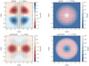 |
Fig. 9. Examples of magnetic field configurations in the halo in the vertical (left panel) and horizontal (right panel) planes. Top row panel: magnetic structure anti-symmetric with respect to the galactic mid-plane (the dipolar symmetry), while the bottom row shows the symmetric magnetic field (quadrupolar symmetry). The strength of the azimuthal magnetic field is shown with colour in the left-hand column whilst the total field strength is colour-coded in the right-hand column. Arrows represent the direction and strength of the magnetic field projected onto the figure plane. |
The eigenfunctions are normalised to have  and
and 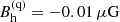 at (s, z) = (8.5, 0.02) kpc in the anti-symmetric and symmetric cases, respectively, so that they have similar maximum magnetic field strengths.
The poloidal magnetic lines (the left-hand panels) have the so-called X shape detected in the halos of some galaxies, especially pronounced in the quadrupolar structure. This is a generic field structure typical of any divergence-free vector field that can be enhanced further by a large-scale velocity shear of the galactic wind or fountain. Unlike the symmetric eigenfunction, the anti-symmetric one has a maximum away from the equator. The position of the maxima depends on the spatial forms of α(r) and V(r); in our case, the rotation speed is independent of z, and α(r) alone controls this feature.
It is not clear which of the two symmetries may dominate in galactic haloes: this depends on the strength of the magnetic coupling between the disc and the halo and between the two hemispheres of the halo. If the disc-halo coupling is strong or the disc disrupts magnetic connection between the two halo hemispheres, the quadrupolar disc field could enforce a symmetric field structure in the halo. Halo fields of mixed parity are also a possibility, but their modelling requires non-linear dynamo solutions rather than superpositions of linear eigenmodes that we use here. The strength of the disc-halo magnetic connection depends on the ratio of the turbulent magnetic diffusivities in the two regions: the larger the value of βh/βd, the weaker the coupling. Existing models of the mean-field dynamo action in galactic disc-halo systems only considered the range βh/βd ≤ 30.
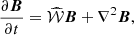
The top two panels of Fig. 10 illustrate how the growth rates and oscillation frequencies of the symmetric and anti-symmetric modes depend on Rαh when all other parameters are fixed to the fiducial values of Table 1. These solutions involve the first four symmetric or anti-symmetric free-decay modes with expansion coefficients shown in the lower half of Fig. 10. As shown in Fig. 10b, both the symmetric and anti-symmetric eigenmodes are typically oscillatory (ImΓ ≠ 0). The fact that ImΓ = 0 for the anti-symmetric mode at Rαh ≳ 10 appears to be an artefact of including only a small number of the free-decay modes into the perturbation series. The series Eq. (59) converges rather slowly (Rädler & Wiedemann 1989; Rädler et al. 1990) and adding a few more terms does not always improve the accuracy (Sokoloff et al. 2008). Therefore, the model for the halo magnetic field that involves only a modest number of modes can reproduce only relatively simple magnetic configurations (and yet quite non-trivial – see Fig. 11). This does not appear to be a serious problem, though, since the scale of the mean magnetic field in galactic haloes is unlikely to be smaller than a few kiloparsecs.
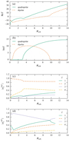 |
Fig. 10. Panel a: growth rates ReΓ and ( panel b) oscillation frequencies ImΓ of the symmetric (solid) and anti-symmetric (dashed) fastest-growing dynamo eigenmodes in a spherical halo as a function of Rαh, with all the remaining parameters fixed at their fiducial values shown in Table 1. Panels c and d: the magnitudes of the expansion coefficients ai in Eq. (59) for the dipolar and quadrupolar modes, respectively. We note that each sharp bend in ReΓ that occurs as Rαh changes is connected with an intersection of two curves ai with distinct values of i. |
 |
Fig. 11. Three-dimensional rendering of a symmetric (quadrupolar) halo field combined with a quadrupolar disc field with two reversals at s = 7 kpc and 12 kpc. The domain is a (17 kpc)3 box. The field lines were seeded uniformly along a diagonal through the box. The arrows show the magnetic field at points randomly sampled within the slice of a thickness 2.5 kpc around the galactic mid-plane (which is indicated by the semi-transparent surface) and are scaled according to the magnitude of the magnetic field. |
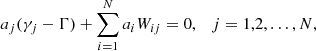
The dependencies of the growth rate and oscillation frequency of the magnetic field on the turnover radius of the rotation curve sv are shown in Fig. 12. Larger values of sv correspond to weaker differential rotation and, therefore, lower growth rates and oscillation frequencies.
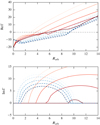 |
Fig. 12. The effect of the form of the rotation curve on the dynamo growth rate ReΓ and oscillation frequency ImΓ of the fastest-growing magnetic field in the spherical halo. The shade of each curve corresponds to the value of the turnover radius of the rotation curve, sv, with the lightest shade for sv = 0.5 kpc and the darkest for sv = 7.5 kpc with the increment of 1.75 kpc (the fiducial value is sv = 3 kpc). Dashed curves are for the anti-symmetric eigenmodes and solid curves show symmetric solutions. |
5. Discussion
Magnetic fields obtained above for the disc and halo are combined by a simple superposition with arbitrary weights. For illustration, we show in Fig. 11 a magnetic structure that has two radial field reversals in the disc (Model B of Fig. 7) and a symmetric (quadrupolar) field in the halo shown in the bottom row of Fig. 9. The complexity of the resulting magnetic structure clearly illustrates the possibilities of the model. The most important limitations of the model in its current form is that it is axially symmetric and does not include galactic outflows. Both can be addressed rather straightforwardly within the framework of this approach. In the following we discuss some applications and extensions of our approach.
5.1. Synthetic radio maps
The model can be used to interpret observations of synchrotron emission and Faraday rotation as soon as the distributions of cosmic ray and thermal electrons have been specified. The total and polarised synchrotron intensities, polarisation angle and Faraday rotation measure can be derived as described in Appendix C. As a simple illustrative example, we assume a uniform distribution for the cosmic-ray electrons, nγ = const in terms of the number density, and adopt exponential profiles for the number density of thermal electrons,
![Mathematical equation: $$ \begin{aligned} n_\mathrm{e} ({s}, z, \phi ) = n_0 \exp \left[-\frac{z}{h({s})}-\frac{{s}}{{s}_\text{ e}}\right], \end{aligned} $$](/articles/aa/full_html/2019/03/aa34642-18/aa34642-18-eq92.gif) (69)
(69)
where h(s) is given by Eq. (3) and se = 3 kpc, is the scale radius of the disc (chosen to be similar to the case of the Milky Way, Binney & Tremaine 2008). Any other model (e.g. Cordes & Lazio 2002) could be used instead but we prefer to avoid exaggerating the amount of detail in the magnetic field model that may arise from details such as spiral arms in more complicated models for ne.
In the top panel Fig. 13, we show the synchrotron emission in a galaxy seen edge-on with the magnetic field of Fig. 11. The other two panels show the polarised emission at two wavelengths, λ = 5 cm and λ = 20 cm, as in C- and L-bands of the VLA used, for example, in the CHANG-ES survey (Irwin et al. 2012). At 5 cm, most of the polarisation signal is dominated by the disc component and localised around the mid-plane of the disc. At longer wavelengths, most of the emission from the galactic plane is depolarised and two conical lobes of about 5 kpc in height are prominent in the halo, similar to the so-called X-shaped structures observed in edge-on galaxies (Wiegert et al. 2015).
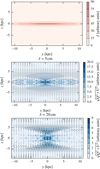 |
Fig. 13. Synchrotron emission produced by the magnetic configuration shown in Fig. 11 with the disc seen edge-on (see the text for other assumptions). Top panel: the total intensity (Stokes parameter I). Middle and bottom panels: the polarised intensity at λ = 5 and λ = 20 cm, respectively. The dashes are perpendicular to the polarisation angle and their lengths are proportional to the fractional polarisation. No correction for random magnetic fields has been made in the fractional polarisation. |
5.2. Evolution of galactic magnetic fields
Another possible application is a simple, approximate model for the evolution of a large-scale magnetic field in a galaxy. In this application, an initial (seed) magnetic field has to be prescribed and then it can be evolved using the growth rates of the magnetic modes derived above. Suitable initial conditions must then be selected. The simplest approach is to assume that all the modes are equally represented in the initial state, that is, Cn independent of n and chosen to obtain an initial large-scale magnetic field of any given strength. A physically better motivated initial magnetic field represents a random field produced by the fluctuation dynamo in a young galaxy or protogalaxy (Poezd et al. 1993). Because of the finite size of the dynamo region, the projection of such a random field onto the dynamo eigenmodes does not vanish. Ruzmaikin et al. (Sect. VII.14 in 1988) estimate the corresponding initial dimensional magnitudes of the radial disc modes as
 (70)
(70)
where b is the root-mean square strength of the random magnetic field b, Nn is the number of the correlation cells of b within a cylindrical annulus of an axial extent 2h, radius s and width δsn, with δsn the radial scale of Qn(s), and l is the scale of b. With δs ≃ sdisc/n, N ≃ hssdisc/(nl3), l = 100 pc, sdisc = 20 kpc, we have
 (71)
(71)
Thus, the seed for the large-scale dynamo due to the small-scale magnetic field favours higher-order modes being proportional to n3/2, because they have smaller scale, and decreases with radius as s−1/2. A plausible estimate is b ≃ 5 μG by analogy with observational estimates for nearby spiral galaxies. Otherwise, if a dependence on the interstellar gas parameters is required, a suitable estimate is
 (72)
(72)
where ρ is the gas density in the diffuse warm interstellar gas and v is the turbulent speed. The standard estimates of the latter are ρ ≃ 1, 7 × 10⁻²⁴ g cm−3 corresponding to the number density of 1 cm−3 and v ≃ 10 km s−1. This yields b ≃ 3 μG.
5.3. Extensions of the model
There are several directions in which the model can be extended. Perhaps most important is to include non-axisymmetric magnetic fields. This is straightforward to implement. In the disc, the local equations of Sect. 3.3 and their solutions remain unchanged but the radial part of the eigenfunction Qn of Sect. 3.4 becomes a function of both radius and azimuth. Solutions for Qm(s, ϕ) were obtained in largely the same manner as above by Baryshnikova et al. (1987), Krasheninnikova et al. (1989), and Bykov et al. (1997), and are reviewed by Ruzmaikin et al. (Sect. VII.8 in 1988) and Krasheninnikova et al. (1990). Introducing non-axisymmetric magnetic fields in the halo would only require that non-axisymmetric free-decay modes are included into the perturbation solution. This is straightforward to do and does not require any significant modification of the formalism of Sect. 4.1.
Another physically important generalisation is the inclusion of galactic outflows and accretion flows, that is, large-scale poloidal velocity fields U. The additional velocity components appear in the perturbation operators. Within the disc, Uz enters the local Eqs. (18) and (19) whereas Us is included in the radial Eq. (40). The modified solutions are discussed by Bardou et al. (2001) and Moss et al. (2000), respectively. In the halo, the poloidal velocity just enters the perturbation operator Eq. (63) without affecting the procedure of perturbation analysis.
The solutions used in the model are kinematic (linear in magnetic field) as they are derived for V, α and β independent of B. The linear nature of the solution is not restrictive in the present context since its aim is to provide a convenient functional basis to parametrise a desired magnetic configuration. On the other hand, Chamandy et al. (2014) show that a wide class of non-linear solutions are well approximated by the marginally stable eigenfunction (i.e., that obtained for ∂B/∂t = 0). Non-linear dynamo effects, leading to solutions sensitive to the gas density and other relevant parameters, can be introduced in the radial thin-disc Eq. (40) as discussed by Poezd et al. (1993), via a non-linear modification (quenching) of the local growth rate which becomes a function of Q:
![Mathematical equation: $$ \begin{aligned} \gamma ({s},Q) = \gamma ({s})\left[ 1- Q^2/B_0^2({s})\right], \end{aligned} $$](/articles/aa/full_html/2019/03/aa34642-18/aa34642-18-eq96.gif)
where γ(s) is the kinematic local growth rate obtained as discussed in Sect. 3.3. Since the time scale of magnetic field evolution in the halo is comparable to 1010 yr (Sect. 4), non-linear dynamo effects are likely to be less important in galactic haloes.
5.4. The GALMAG software package
The model presented in this paper has been implemented as the Python software package GALMAG1 (Rodrigues 2018), which is publicly available under the GNU General Public License v3. Further details can be found in the on-line code documentation2, which includes a tutorial.
Since GALMAG uses Python objects of the D2O package (Steininger et al. 2016) instead of regular NUMPY arrays, when it is invoked using MPI, all the array operations are automatically performed in parallel. As a stand-alone package, it can synthesise three-dimensional magnetic field structures from a provided set of expansion coefficients and compute synthetic maps of the Stokes parameters of synchrotron emission and Faraday rotation.
A more flexible use of GALMAG is to employ it in modular magnetic field optimisation frameworks like the IMAGINE pipeline (Steininger et al. 2018; Steininger 2018), where it serves as a magnetic field generator and is interfaced to multi-purpose observable generators, such as the HAMMURABI code3 (Waelkens et al. 2009). This allows us to not only compute maps of observables from any point of view and thus to compare with observations, but also provides sophisticated sampling techniques to optimise the GALMAG parameters.
6. Conclusions
We have presented an approach to develop parametrised models for large scale magnetic fields of the Milky Way and other disc galaxies based on fundamental equations of magnetic field generation and evolution. Implemented in the software package GALMAG, it is designed to be used in interpretations of observations of Faraday rotation, synchrotron and dust emission, and other observational tracers. In this paper, we have presented the basic formalism of the approach, and demonstrated its capabilities in illustrative examples.
The model is based on the expansion of the large-scale magnetic field over a basis of eigenfunctions of the mean-field dynamo Eq. (1), and the standard induction equation is its special case obtained for α = 0. As long as the functional basis is complete, any magnetic structure, whether or not produced by the dynamo, can be represented as a superposition of the eigenfunctions. Therefore, an alternative use of the magnetic field model is to represent any magnetic configuration of interest in terms of a relatively small number of parameters. The resulting magnetic field is physically realisable, being a solution of the induction equation or its modification with α ≠ 0, as desired. Furthermore, the fact that the model parameters have clear physical meaning would help to refine it so as to satisfy any additional constraints. Magnetic fields of the model are obtained in the form of series expansions, and the series can be truncated to achieve the desired amount of detail in the resulting solution.
The novelty and strength of our approach lies in advancing both the flexibility and physical plausibility of GMF models. It will be useful in Bayesian optimization machines, which seek among many reasonable morphological approaches to the GMF structure the one that gives the best results both in terms of physical plausibility and the explanation of existing data.
Acknowledgments
We have benefited from fruitful discussions with the members of the ISSI International Team 323, Bayesian modeling of the Galactic magnetic field constrained by space- and ground-based radio-millimetre and ultra-high energy cosmic ray data (http://www.issibern.ch/teams/bayesianmodel/), and the IMAGINE Consortium (https://www.astro.ru.nl/imagine/). Special thanks are due to Torsten Enßlin, Marijke Haverkorn, Jens Jasche and Andrew Fletcher for their useful comments, and Theo Steininger for help with the software development and the D2O Python package AS, LFSR and JPR acknowledge financial support and hospitality of the International Space Science Institute (ISSI) in Bern, Switzerland. AS and LFSR are supported by STFC (ST/N000900/1, Project 2), and AS and PB are supported by the Leverhulme Trust (RPG-2014-427). This research has made use of NASA’s Astrophysics Data System.
References
- Bardou, A., von Rekowski, B., Dobler, W., Brandenburg, A., & Shukurov, A. 2001, A&A, 370, 635 [NASA ADS] [CrossRef] [EDP Sciences] [Google Scholar]
- Baryshnikova, Yu, Shukurov, A., Ruzmaikin, A., & Sokoloff, D. D. 1987, A&A, 177, 27 [NASA ADS] [Google Scholar]
- Beck, R. 2007, A&A, 470, 539 [NASA ADS] [CrossRef] [EDP Sciences] [Google Scholar]
- Beck, R. 2015, A&ARv, 24, 4 [NASA ADS] [CrossRef] [Google Scholar]
- Beck, R., Brandenburg, A., Moss, D., Shukurov, A., & Sokoloff, D. 1996, ARA&A, 34, 155 [NASA ADS] [CrossRef] [Google Scholar]
- Bendre, A., Gressel, O., & Elstner, D. 2015, Astron. Nachr., 336, 991 [NASA ADS] [CrossRef] [Google Scholar]
- Binney, J., & Tremaine, S. 2008, Galactic Dynamics, 2nd edn. (Princeton, USA: Princeton University Press) [Google Scholar]
- Boulanger, F., Enßlin, T., Fletcher, A., et al. 2018, J. Cosmol. Astro-Part. Phys., 8, 049 [NASA ADS] [CrossRef] [Google Scholar]
- Brandenburg, A., & Subramanian, K. 2005, Phys. Rep., 417, 1 [NASA ADS] [CrossRef] [Google Scholar]
- Bykov, A., Popov, V., Shukurov, A., & Sokoloff, D. 1997, MNRAS, 292, 1 [NASA ADS] [CrossRef] [Google Scholar]
- Case, G. L., & Bhattacharya, D. 1998, ApJ, 504, 761 [Google Scholar]
- Chamandy, L., Shukurov, A., Subramanian, K., & Stoker, K. 2014, MNRAS, 443, 1867 [NASA ADS] [CrossRef] [Google Scholar]
- Clemens, D. P. 1985, ApJ, 295, 422 [NASA ADS] [CrossRef] [Google Scholar]
- Cordes, J. M., & Lazio, T. J. W. 2002, ArXiv e-prints [arXiv:astro-ph/0207156] [Google Scholar]
- Dickey, J. M., & Lockman, F. J. 1990, ARA&A, 28, 215 [NASA ADS] [CrossRef] [MathSciNet] [Google Scholar]
- Ferrière, K., & Terral, P. 2014, A&A, 561, A100 [NASA ADS] [CrossRef] [EDP Sciences] [Google Scholar]
- Gressel, O., Elstner, D., Ziegler, U., & Rüdiger, G. 2008a, A&A, 486, L35 [NASA ADS] [CrossRef] [EDP Sciences] [Google Scholar]
- Gressel, O., Ziegler, U., Elstner, D., & Rüdiger, G. 2008b, Astron. Nachr., 329, 619 [NASA ADS] [CrossRef] [Google Scholar]
- Haverkorn, M. 2015, Astrophys. Space Sci. Lib., 407, 483 [NASA ADS] [CrossRef] [Google Scholar]
- Hollins, J. F., Sarson, G. R., Shukurov, A., Fletcher, A., & Gent, F. A. 2017, ApJ, 850, 4 [NASA ADS] [CrossRef] [Google Scholar]
- Hopkins, P. F., Wetzel, A., Kereš, D., et al. 2018, MNRAS, 480, 800 [NASA ADS] [CrossRef] [Google Scholar]
- Irwin, J., Beck, R., Benjamin, R. A., et al. 2012, AJ, 144, 43 [NASA ADS] [CrossRef] [Google Scholar]
- Jaffe, T. R., Leahy, J. P., Banday, A. J., et al. 2010, MNRAS, 401, 1013 [NASA ADS] [CrossRef] [Google Scholar]
- Jansson, R., & Farrar, G. R. 2012a, ApJ, 757, 14 [NASA ADS] [CrossRef] [Google Scholar]
- Jansson, R., & Farrar, G. R. 2012b, ApJ, 761, L11 [NASA ADS] [CrossRef] [Google Scholar]
- Ji, Y., Cole, L., Bushby, P., & Shukurov, A. 2014, Geophys. Astrophys. Fluid Dyn., 108, 568 [NASA ADS] [CrossRef] [Google Scholar]
- Kalberla, P. M. W., & Kerp, J. 2009, ARA&A, 47, 27 [NASA ADS] [CrossRef] [Google Scholar]
- Kalberla, P. M. W., Westphalen, G., Mebold, U., Hartmann, D., & Burton, W. B. 1998, A&A, 332, L61 [NASA ADS] [Google Scholar]
- Kotera, K., & Olinto, A. V. 2011, ARA&A, 49, 119 [NASA ADS] [CrossRef] [Google Scholar]
- Krasheninnikova, Yu, Shukurov, A., Ruzmaikin, A., & Sokoloff, D. 1989, A&A, 213, 19 [NASA ADS] [Google Scholar]
- Krasheninnikova, Yu, Ruzmaikin, A., Sokoloff, D., & Shukurov, A. 1990, Geophys. Astrophys. Fluid Dyn., 50, 131 [NASA ADS] [CrossRef] [Google Scholar]
- Krause, F., & Rädler, K. H. 1980, Mean-Field Magnetohydrodynamics and Dynamo Theory (Oxford: Pergamon Press) [Google Scholar]
- Lockman, F. J. 1984, ApJ, 283, 90 [NASA ADS] [CrossRef] [Google Scholar]
- Mac Low, M.-M., & Klessen, R. S. 2004, Rev. Mod. Phys., 76, 125 [NASA ADS] [CrossRef] [Google Scholar]
- Mao, S. A., Zweibel, E., Fletcher, A., Ott, J., & Tabatabaei, F. 2015, ApJ, 800, 92 [NASA ADS] [CrossRef] [Google Scholar]
- McKee, C. F., & Ostriker, J. P. 1977, ApJ, 218, 148 [NASA ADS] [CrossRef] [Google Scholar]
- Moffatt, H. K. 1978, Magnetic Field Generation in Electrically Conducting Fluids (Cambridge: Cambridge University Press) [Google Scholar]
- Mollerach, S., & Roulet, E. 2018, Nucl. Phys., 98, 85 [Google Scholar]
- Moss, D., Shukurov, A., & Sokoloff, D. 2000, A&A, 358, 1142 [NASA ADS] [Google Scholar]
- Pakmor, R., & Springel, V. 2013, MNRAS, 432, 176 [NASA ADS] [CrossRef] [Google Scholar]
- Pakmor, R., Gómez, F. A., Grand, R. J. J., et al. 2017, MNRAS, 469, 3185 [NASA ADS] [CrossRef] [Google Scholar]
- Planck Collaboration XLII. 2016, A&A, 596, A103 [NASA ADS] [CrossRef] [EDP Sciences] [Google Scholar]
- Planck Collaboration XI. 2019, A&A, in press, DOI: 10.1051/0004-6361/201832618 [Google Scholar]
- Poezd, A., Shukurov, A., & Sokoloff, D. 1993, MNRAS, 264, 285 [NASA ADS] [CrossRef] [Google Scholar]
- Priklonsky, V., Shukurov, A., Sokoloff, D., & Soward, A. 2000, Geophys. Astrophys. Fluid Dyn., 93, 97 [NASA ADS] [CrossRef] [Google Scholar]
- Rädler, K.-H., Wiedemann, E., Brandenburg, A., Meinel, R., & Tuominen, I. 1990, A&A, 239, 413 [NASA ADS] [Google Scholar]
- Rädler, K.-H., & Wiedemann, E. 1989, Geophys. Astrophys. Fluid Dyn., 49, 71 [NASA ADS] [CrossRef] [Google Scholar]
- Reyes, R., Mandelbaum, R., Gunn, J. E., Pizagno, J., & Lackner, C. N. 2011, MNRAS, 417, 2347 [NASA ADS] [CrossRef] [Google Scholar]
- Rodrigues, L. F. S. 2018, GalMag: A Python Tool for Computing Realistic Galactic Magnetic Fields, DOI: 10.5281/zenodo.1135245 [Google Scholar]
- Rodrigues, L. F. S., Sarson, G. R., Shukurov, A., Bushby, P. J., & Fletcher, A. 2016, ApJ, 816, 2 [NASA ADS] [CrossRef] [Google Scholar]
- Ruzmaikin, A. A., Sokoloff, D. D., & Shukurov, A. M. 1980, Magnetohydrodynamics, 16, 15 [Google Scholar]
- Ruzmaikin, A. A., Shukurov, A. M., & Sokoloff, D. D. 1988, Magnetic Fields of Galaxies (Dordrecht: Kluwer) [CrossRef] [Google Scholar]
- Schaller, M., Frenk, C. S., Bower, R. G., et al. 2015, MNRAS, 451, 1247 [NASA ADS] [CrossRef] [Google Scholar]
- Shukurov, A. 2007, in Mathematical Aspects of Natural Dynamos, eds. E. Dormy, & A. M. Soward (Boca Raton, FL: Taylor and Francis), 319 [Google Scholar]
- Shukurov, A., & Sokoloff, D. 2008, in Dynamos: Lecture Notes of the Les Houches Summer School 2007, eds. P. Cardin, & L. G. Cugliandolo (Elsevier Science), 251 [Google Scholar]
- Shukurov, A., & Subramanian, K. 2018, Astrophysical Magnetic Fields: from Galaxies to the Early Universe (Cambridge: Cambridge University Press) [Google Scholar]
- Sokoloff, D. D., Nefedov, S. N., Ermash, A. A., & Lamzin, S. A. 2008, Astron. Lett., 34, 761 [NASA ADS] [CrossRef] [Google Scholar]
- Steininger, T. 2018, Astrophysics Source Code Library [record ascl:1803.007] [Google Scholar]
- Steininger, T., Enßlin, T. A., Greiner, M., et al. 2018, ArXiv e-prints [arXiv:1801.04341] [Google Scholar]
- Steininger, T., Greiner, M., Beaujean, F., & Enßlin, T. 2016, J. Big Data, 3, 17 [CrossRef] [Google Scholar]
- Sun, X. H., Reich, W., Waelkens, A., & Enßlin, T. A. 2008, A&A, 477, 573 [NASA ADS] [CrossRef] [EDP Sciences] [Google Scholar]
- Terral, P., & Ferrière, K. 2017, A&A, 600, A29 [NASA ADS] [CrossRef] [EDP Sciences] [Google Scholar]
- Van Eck, C. L., Brown, J. C., Stil, J. M., et al. 2011, ApJ, 728, 97 [NASA ADS] [CrossRef] [Google Scholar]
- Waelkens, A., Jaffe, T., Reinecke, M., Kitaura, F. S., & Enßlin, T. A. 2009, A&A, 495, 697 [NASA ADS] [CrossRef] [EDP Sciences] [Google Scholar]
- Wiegert, T., Irwin, J., Miskolczi, A., et al. 2015, AJ, 150, 81 [NASA ADS] [CrossRef] [Google Scholar]
- Willis, A. P., Shukurov, A., Soward, A. M., & Sokoloff, D. 2004, Geophys. Astrophys. Fluid Dyn., 98, 345 [NASA ADS] [CrossRef] [Google Scholar]
- Zschaechner, L. K., Rand, R. J., & Walterbos, R. 2015, ApJ, 799, 61 [NASA ADS] [CrossRef] [Google Scholar]
Appendix A: Spherical free-decay modes
For axisymmetric free-decay modes, a solution to Eq. (60) is obtained in terms of scalar potentials, as discussed by Krause & Rädler (1980) and Moffatt (1978). For the reader’s convenience, we present an outline of the solution. Any magnetic field B can be represented as the sum of a poloidal field ∇ × AP, where AP is its vector potential, and a toroidal field BT:
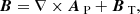 (A.1)
(A.1)
and ∇ ⋅ B = 0 provided
 (A.2)
(A.2)
where r is the position vector normalised such that r = 1 is the halo surface (r = rh in dimensional variables) and S and T are known as the scalar potentials. In terms of the scalar potentials and assuming axial symmetry, Eq. (60) reduces in spherical coordinates (r, θ, ϕ) to
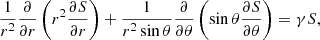 (A.3)
(A.3)
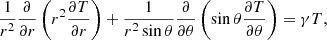 (A.4)
(A.4)
for r < 1 and,
 (A.5)
(A.5)
with the vacuum boundary conditions
![Mathematical equation: $$ \begin{aligned}[S]=[\partial {S}/ \partial {r}]=[T]=0 \ \text{ at}\ r=1, \end{aligned} $$](/articles/aa/full_html/2019/03/aa34642-18/aa34642-18-eq102.gif) (A.6)
(A.6)
where [X] denotes the jump of X, and [X]=0 means continuity. We also require both potentials to be finite at r = 0.
The potentials satisfy identical equations at r < 1, so consider this equation for G equal to either S or T,
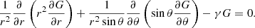 (A.7)
(A.7)
Using separation of variables, G(r, θ)=R(r)Θ(θ), Bessel’s equation is obtained in r and Legendre’s equation in θ, with the separation constant n(n + 1) (n = 1, 2, 3, …):
![Mathematical equation: $$ \begin{aligned} r^{2}\frac{\mathrm{d} ^2R}{\mathrm{d} r^2}+2r\frac{\mathrm{d} R}{\mathrm{d} r}-[{\gamma }r^{2}+n(n+1)]R=0, \end{aligned} $$](/articles/aa/full_html/2019/03/aa34642-18/aa34642-18-eq104.gif) (A.8)
(A.8)
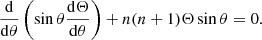 (A.9)
(A.9)
In terms of  and Q(x)=x1/2R(x) in Eq. (A.8) and x = cosθ in Eq. (A.9), we have
![Mathematical equation: $$ \begin{aligned} x^2\frac{\mathrm{d} ^2Q}{\mathrm{d} x^{2}}+x\frac{\mathrm{d} Q}{\mathrm{d} x}+\left[x^2-\left(n+\tfrac{1}{2}\right)^2\right]Q=0, \end{aligned} $$](/articles/aa/full_html/2019/03/aa34642-18/aa34642-18-eq107.gif) (A.10)
(A.10)
![Mathematical equation: $$ \begin{aligned} \frac{\mathrm{d} }{\mathrm{d} x}\left[(1-x^2){\frac{\mathrm{d} \Theta }{\mathrm{d} x}} \right]+n(n+1)\Theta =0. \end{aligned} $$](/articles/aa/full_html/2019/03/aa34642-18/aa34642-18-eq108.gif) (A.11)
(A.11)
Non-singular solutions of Eqs. (A.3) and (A.4) then follow as
 (A.12)
 (A.13)
where
 (A.14)
with constants cnl,
 (A.15)
and ξnl are solutions to (A.18). The factor rh in Eq. (A.13) is introduced to ensure dimensional consistency when obtaining the magnetic field from these potentials. The boundary conditions (A.6) reduce to
 (A.16)
where dn are constants. Eliminating dn, the boundary conditions for Snl reduce to the recurrence relation
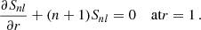 (A.17)
Together with the requirement that Tnl and Snl do not vanish simultaneously, this gives
 (A.18)
which determines the admissible values for ξnl, and  yields the decay rates γnl given in Table A.1.
For l odd, Jn − 1/2(ξnl)=0 for all n. Hence, Tnl = 0 for l odd. Conversely, when l is even, Jn + 1/2(ξnl)=0 for all n. Hence, Snl = 0 for l even. The solutions satisfying the boundary conditions can be written as follows:
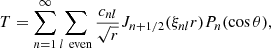 (A.19a)
 (A.19b)
where cnl and dnl are constants. Individual terms in the sums are arranged according to increasing magnitude of the decay rates, |γnl|.
Decay rates of spherical free-decay modes, γnl.
The free-decay modes form two separate families based on their symmetry about the equator θ = π/2, the anti-symmetric (dipolar) and symmetric (quadrupolar) ones. The anti-symmetric modes, denoted with superscript (d), occur when both n and l are either odd or even, whilst the symmetric modes that have superscript (q) occur otherwise.
Explicit forms of a few of the lowest free-decay modes are given in the next section, each normalised to
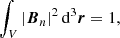 (A.20)
where the integral is taken over the sphere r ≤ 1, to form an orthonormal set. Although each eigenmode is either poloidal or toroidal, their superpositions Eq. (A.20) necessarily contain both poloidal and toroidal parts: purely toroidal and purely poloidal fields cannot sustain Ohmic dissipation and unavoidably decay.
A.1. Symmetric modes
The four leading quadrupolar free-decay modes are shown in the upper row of Fig. 8. The quadrupolar mode of the slowest decay has (n, l)=(2, 1) and is poloidal,
![Mathematical equation: $$ \begin{aligned} {\boldsymbol{B}}_1^\text{(q)}=A_1 \left( \frac{Q_1(r)}{r}(3\cos ^2\theta -1),\ -\frac{\sin \theta \,\cos \theta }{r}\frac{\mathrm{d} }{\mathrm{d} r}[rQ_1(r)],\ 0\right), \end{aligned} $$](/articles/aa/full_html/2019/03/aa34642-18/aa34642-18-eq120.gif) (A.21)
(A.21)
where A1 ≈ 0.662 and
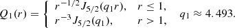 (A.22)
The next mode, (n, l)=(1, 2), is toroidal and has the same eigenvalue,
 (A.23)
where A2 ≈ 1.330 and
 (A.24)
The modes  and
and  , poloidal and toroidal respectively, also form a doublet with the common eigenvalue and correspond to (n, l)=(4, 1) and (n, l)=(3, 2), respectively:
![Mathematical equation: $$ \begin{aligned} {\boldsymbol{B}}_3^\text{(q)}=A_3\left(-20 \frac{Q_3(r)}{r} S_1(\theta ),\ -r^{-1}\frac{\mathrm{d} }{\mathrm{d} r}[rQ_3(r)]\frac{\mathrm{d} S_1(\theta )}{\mathrm{d} \theta },\ 0 \right), \end{aligned} $$](/articles/aa/full_html/2019/03/aa34642-18/aa34642-18-eq126.gif) (A.25)
(A.25)
where A3 ≈ 0.133, S1(θ)=35cos4θ − 30cos2θ + 3 and
 (A.26)
and
 (A.27)
where A4 ≈ 0.763, S2(θ)=5cos3θ − 3cosθ and
 (A.28)
A.2. Anti-symmetric modes
The spherical components of magnetic field in a few leading anti-symmetric modes have the following form, illustrated in the bottom row of Fig. 8.
The mode that decays most slowly is poloidal, with (n, l)=(1, 1):
![Mathematical equation: $$ \begin{aligned} {\boldsymbol{B}}_1^\mathrm{(d)} =C_1\left(\frac{2}{r}Q_1(r)\,\cos \theta , \ -\frac{\sin \theta }{r}\frac{\mathrm{d} }{\mathrm{d} r}[rQ_1(r)], \ 0 \right), \end{aligned} $$](/articles/aa/full_html/2019/03/aa34642-18/aa34642-18-eq130.gif) (A.29)
(A.29)
where C1 ≈ 0.346 and
 (A.30)
The next two modes  and
and  , poloidal and toroidal with (n, l)=(3, 1) and (n, l)=(2, 2), respectively, form a degenerate pair:
![Mathematical equation: $$ \begin{aligned} {\boldsymbol{B}}_2^\mathrm{(d)}&= C_2 \left(\frac{2\cos \theta }{r} (5\cos 2\theta -1)Q_2(r)\right., \nonumber \\&\quad \left.-\frac{\sin \theta }{r}(5\cos ^2\theta -1) \frac{\mathrm{d} }{\mathrm{d} r}\left[rQ_2(r)\right], \ 0\right), \end{aligned} $$](/articles/aa/full_html/2019/03/aa34642-18/aa34642-18-eq134.gif) (A.31)
(A.31)
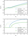 |
Fig. A.1. Growth rates ReΓ and oscillation frequencies ImΓ of the symmetric and anti-symmetric fastest-growing eigenmodes of the spherical αω-dynamo as a function of Rαh with the remaining parameters fixed at their fiducial values. Dashed curves show the results obtained for the α2ω-dynamo, whereas solid curves are for the αω-dynamo. |
where C2 ≈ 0.250 and
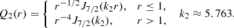 (A.32)
The toroidal mode of the doublet has the form
 (A.33)
where C3 ≈ 3.445 and
 (A.34)
The fourth antisymmetric mode is also poloidal, with (n, l)=(1, 3):
![Mathematical equation: $$ \begin{aligned} {\boldsymbol{B}}_4^\mathrm{(d)} =C_4\left(\frac{2}{r}Q_4(r)\,\cos \theta , \ -\frac{1}{r}\frac{\mathrm{d} }{\mathrm{d} r}[rQ_4(r)]\,\sin \theta , \ 0 \right), \end{aligned} $$](/articles/aa/full_html/2019/03/aa34642-18/aa34642-18-eq138.gif) (A.35)
(A.35)
where C4 ≈ 0.244 and
 (A.36)
Appendix B: The αω-dynamo approximation for the halo
In the main part of this paper, we use an α2ω-dynamo model for the halo, where the toroidal magnetic field is produced from the poloidal one by both differential rotation and the α-effect. The contribution of the α2-dynamo to the generation of the toroidal field is usually weaker and therefore often neglected to simplify the solutions. To assess the consequences of this approximation, here we provide solutions of the αω-dynamo in the halo which should be compared with results presented in Sect. 4.3.
For the αω-dynamo, the operator defined in Eq. (63) is simplified to
![Mathematical equation: $$ \begin{aligned} {\widehat{\mathcal{W} }}{\boldsymbol{B}}={R_{\alpha \text{ h}}}\left(\nabla \times ({\alpha }{\boldsymbol{B}})-[ \nabla \times ({\alpha }{\boldsymbol{B}})]_{\phi }\right)+{R_{\omega \text{ h}}}\nabla \times ({\boldsymbol{V}} \times {\boldsymbol{B}}), \end{aligned} $$](/articles/aa/full_html/2019/03/aa34642-18/aa34642-18-eq140.gif) (B.1)
(B.1)
thus removing the contribution of the α-effect to the azimuthal magnetic field. In Fig. A.1, similar to Fig. 10, we show the resulting eigenvalues and expansion coefficients of the perturbation solution. The difference between the two solutions is noticeable.
The α2-dynamo is negligible in comparison with the αω mechanism when |Rω/Rα|≫1 or even  (Ruzmaikin et al. 1980). For the fiducial value of parameters, |Rω/Rα|≃140 in the disc and 50–100 in the halo (and |Rωh/Rαh2 = 10–50). Thus, unlike the case of galactic discs with strong differential rotation, the αω-approximation cannot be recommended for the halo because it neglects a potentially important part of the dynamo mechanism.
Appendix C: Synchrotron emission and Faraday rotation
For the line of sight along the x-axis of a Cartesian reference frame r = (x, y, z), the synchrotron emissivity at a wavelength λ is derived as
![Mathematical equation: $$ \begin{aligned} \epsilon ({\boldsymbol{r}},\lambda ) \propto [B_y^2({\boldsymbol{r}})+B_z^2({\boldsymbol{r}})]^{(\kappa +1)/4} \lambda ^{(\kappa -1)/2}, \end{aligned} $$](/articles/aa/full_html/2019/03/aa34642-18/aa34642-18-eq142.gif) (C.1)
(C.1)
assuming a uniform distribution of cosmic ray electrons and the cosmic ray energy spectrum N(E) dE ∝ E−κ dE with κ = 3. The Stokes parameters are computed as
 (C.2)
(C.2)
![Mathematical equation: $$ \begin{aligned} Q(y,z,\lambda )&=p_0 \int _{-\infty }^\infty \epsilon (x^{\prime },y,z,\lambda )\, \cos [2\psi (x^{\prime },y,z)]\,{\mathrm{d} } x^{\prime }, \end{aligned} $$](/articles/aa/full_html/2019/03/aa34642-18/aa34642-18-eq144.gif) (C.3)
(C.3)
![Mathematical equation: $$ \begin{aligned} U(y,z,\lambda )&= p_0\int _{-\infty }^\infty \epsilon (x^{\prime },y,z,\lambda )\, \sin [2\psi (x^{\prime },y,z)]\,{\mathrm{d} } x^{\prime }, \end{aligned} $$](/articles/aa/full_html/2019/03/aa34642-18/aa34642-18-eq145.gif) (C.4)
(C.4)
with the intrinsic polarisation degree p0 = 0.75, and the local polarisation angle ψ(r) is obtained from
![Mathematical equation: $$ \begin{aligned} \psi ({\boldsymbol{r}}) =&\frac{\pi }{2}+\arctan \left[ \frac{B_z({\boldsymbol{r}})}{B_y({\boldsymbol{r}})}\right]\nonumber \\&\;\;+ 0.81{R_{\alpha \text{ d}}} \left(\frac{\lambda }{1\,\mathrm{m}}\right)^2\int _x^{\infty } \frac{n_\mathrm{e} (x^{\prime },y,z)}{1{\,\mathrm{cm}}^{-3}}\, \frac{B_x({\boldsymbol{r}}^{\prime })}{1{\,\mu \mathrm{G}}}\, \frac{{\mathrm{d} } x^{\prime }}{1\,\mathrm{pc}}, \end{aligned} $$](/articles/aa/full_html/2019/03/aa34642-18/aa34642-18-eq146.gif) (C.5)
(C.5)
where the thermal electron density ne(r) is given by Eq. (69) in both the disc and the halo. The polarised intensity, observed polarisation angle and fractional polarisation follow as
 (C.6)
(C.6)
The Faraday rotation measure is calculated as RM = ∂Ψ/∂(λ2).
All Tables
All Figures
|
Fig. 1. Two choices for the rotation curve discussed in the text (upper panel) and the corresponding velocity shear rate S = sdΩ/ds (lower panel): the Milky Way rotation curve obtained from CO observations by Clemens (1985; solid) and a simpler rotation curve given by Eq. (2) (dashed). |
| In the text | |
|
Fig. 2. Comparison of the local quadrupolar eigenfunctions for 𝒟 = −20 (upper panel) and −50 (middle panel) obtained from numerical solution of the local Eqs. (21) and (22) with the approximate eigenfunctions Eqs. (29) and (30): bϕ from the numerical solution are shown solid (red) and bs, dashed (blue); their approximate counterparts are shown with dotted curves of the matching colour. The eigenfunctions are normalised to bϕ(0) = 1. Bottom panel: numerical (black, solid) and approximate, Eqs. (31) (red, dashed), solutions for the local growth rate as a function of the local dynamo number. |
| In the text | |
|
Fig. 3. Radial profiles of the local dynamo number (upper panel) and the local growth rate of the quadrupolar solutions (lower panel) for the flat rotation curve Eq. (2) (solid) and for the MW rotation curve of Clemens (1985; dashed). Upper panel: critical dynamo number 𝒟c ≈ −π3/4 is shown dotted for reference. |
| In the text | |
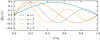 |
Fig. 4. Four leading eigenmodes Qn(s) of the radial Eq. (40) given by Eq. (43). |
| In the text | |
|
Fig. 6. Number and positions of magnetic field reversals along the disc radius, for a magnetic field constructed by a superposition of the first three fastest growing eigenfunctions, Qn(s) with n = 1, 2, 3, for the fiducial choice of parameters shown in Table 1. Left-hand panel: number of the field reversals (colour coded as indicated with the colour bar on the right of the panel) for various ratios of the expansion coefficients Cn/C1. Middle and right-hand panels: galactocentric distances of the inner and outer reversal, srev,1 and srev,2 respectively, colour coded with the colour bar to the right of each panel. White colour indicates the absence of the corresponding reversal. |
| In the text | |
|
Fig. 7. Two examples of the disc magnetic field with radial reversals. Top panels: field strength in the galactic mid-plane is shown colour coded with arrows showing the direction and strength of the magnetic field projected onto the mid-plane. Model A, shown in (panel a), has a reversal at s = 7 kpc and corresponds to the same field as in the bottom right panel of Fig. 5. Model B, shown in (panel b), has the same parameters except for having two reversals at s = 7 and 12 kpc. Panel c: azimuthal magnetic field in the two models. Panel d: vertical cross-section of Model B is shown, with the magnitude of azimuthal magnetic field indicated with colour and arrows showing the projection of the magnetic field onto the (xz)-plane. |
| In the text | |
|
Fig. 5. Sensitivity of the magnetic field structure to the rotation curve and disc flaring, illustrated with magnetic fields constructed using fiducial parameters and (C1, C2) = (4.6 μG, −1.6 μG). The strength of the azimuthal component of the magnetic field is colour coded, while arrows indicate the direction and strength of the poloidal magnetic field. Details of the disc models are indicated above each frame and the disc scale height is indicated with a dotted line on the left and a dashed line on the right. Strong differential rotation near the galactic centre leads to a strong magnetic field, especially in a flat disc. In a flared disc, which is thinner at small s, the field strength near the galactic centre is reduced but the outer region has a stronger field. |
| In the text | |
|
Fig. 8. Eight spherical free-decay eigenfunctions Bi of the smallest decay rates. Each mode is either purely toroidal or purely poloidal. Top row: modes symmetric with respect to the mid-plane z = 0 (quadrupolar modes), while the modes in the bottom row are anti-symmetric (dipolar). For the poloidal modes, arrows represent the projection of the magnetic field on the (xy)-plane. For the toroidal modes, contours show the strength of the azimuthal component of the magnetic field with the normalisation Eq. (A.20). The decay rate of each mode γ is shown at the top of each panel. |
| In the text | |
|
Fig. 9. Examples of magnetic field configurations in the halo in the vertical (left panel) and horizontal (right panel) planes. Top row panel: magnetic structure anti-symmetric with respect to the galactic mid-plane (the dipolar symmetry), while the bottom row shows the symmetric magnetic field (quadrupolar symmetry). The strength of the azimuthal magnetic field is shown with colour in the left-hand column whilst the total field strength is colour-coded in the right-hand column. Arrows represent the direction and strength of the magnetic field projected onto the figure plane. |
| In the text | |
|
Fig. 10. Panel a: growth rates ReΓ and ( panel b) oscillation frequencies ImΓ of the symmetric (solid) and anti-symmetric (dashed) fastest-growing dynamo eigenmodes in a spherical halo as a function of Rαh, with all the remaining parameters fixed at their fiducial values shown in Table 1. Panels c and d: the magnitudes of the expansion coefficients ai in Eq. (59) for the dipolar and quadrupolar modes, respectively. We note that each sharp bend in ReΓ that occurs as Rαh changes is connected with an intersection of two curves ai with distinct values of i. |
| In the text | |
|
Fig. 11. Three-dimensional rendering of a symmetric (quadrupolar) halo field combined with a quadrupolar disc field with two reversals at s = 7 kpc and 12 kpc. The domain is a (17 kpc)3 box. The field lines were seeded uniformly along a diagonal through the box. The arrows show the magnetic field at points randomly sampled within the slice of a thickness 2.5 kpc around the galactic mid-plane (which is indicated by the semi-transparent surface) and are scaled according to the magnitude of the magnetic field. |
| In the text | |
|
Fig. 12. The effect of the form of the rotation curve on the dynamo growth rate ReΓ and oscillation frequency ImΓ of the fastest-growing magnetic field in the spherical halo. The shade of each curve corresponds to the value of the turnover radius of the rotation curve, sv, with the lightest shade for sv = 0.5 kpc and the darkest for sv = 7.5 kpc with the increment of 1.75 kpc (the fiducial value is sv = 3 kpc). Dashed curves are for the anti-symmetric eigenmodes and solid curves show symmetric solutions. |
| In the text | |
|
Fig. 13. Synchrotron emission produced by the magnetic configuration shown in Fig. 11 with the disc seen edge-on (see the text for other assumptions). Top panel: the total intensity (Stokes parameter I). Middle and bottom panels: the polarised intensity at λ = 5 and λ = 20 cm, respectively. The dashes are perpendicular to the polarisation angle and their lengths are proportional to the fractional polarisation. No correction for random magnetic fields has been made in the fractional polarisation. |
| In the text | |
|
Fig. A.1. Growth rates ReΓ and oscillation frequencies ImΓ of the symmetric and anti-symmetric fastest-growing eigenmodes of the spherical αω-dynamo as a function of Rαh with the remaining parameters fixed at their fiducial values. Dashed curves show the results obtained for the α2ω-dynamo, whereas solid curves are for the αω-dynamo. |
| In the text | |
Current usage metrics show cumulative count of Article Views (full-text article views including HTML views, PDF and ePub downloads, according to the available data) and Abstracts Views on Vision4Press platform.
Data correspond to usage on the plateform after 2015. The current usage metrics is available 48-96 hours after online publication and is updated daily on week days.
Initial download of the metrics may take a while.