| Issue |
A&A
Volume 623, March 2019
|
|
|---|---|---|
| Article Number | A161 | |
| Number of page(s) | 22 | |
| Section | Planets and planetary systems | |
| DOI | https://doi.org/10.1051/0004-6361/201834384 | |
| Published online | 27 March 2019 | |
Effects of a fully 3D atmospheric structure on exoplanet transmission spectra: retrieval biases due to day–night temperature gradients
1
Laboratoire d’astrophysique de Bordeaux, Université de Bordeaux, CNRS, B18N, allée Geoffroy Saint-Hilaire, 33615 Pessac, France
e-mail: This email address is being protected from spambots. You need JavaScript enabled to view it.
2
Department of Physics and Astronomy, University College London (UCL), UK
3
LESIA, Observatoire de Paris, PSL Research University, CNRS, Sorbonne Université, Université Diderot Paris, Sorbonne Paris Cité, 92195 Meudon, France
Received:
5
October
2018
Accepted:
23
January
2019
Abstract
Transmission spectroscopy provides us with information on the atmospheric properties at the limb, which is often intuitively assumed to be a narrow annulus around the planet. Consequently, studies have focused on the effect of atmospheric horizontal heterogeneities along the limb. Here we demonstrate that the region probed in transmission – the limb – actually extends significantly towards the day and night sides of the planet. We show that the strong day–night thermal and compositional gradients expected on synchronous exoplanets create sufficient heterogeneities across the limb that result in important systematic effects on the spectrum and bias its interpretation. To quantify these effects, we developed a 3D radiative-transfer model able to generate transmission spectra of atmospheres based on 3D atmospheric structures. We first apply this tool to a simulation of the atmosphere of GJ 1214 b to produce synthetic JWST observations and show that producing a spectrum using only atmospheric columns at the terminator results in errors greater than expected noise. This demonstrates the necessity for a real 3D approach to model data for such precise observatories. Secondly, we investigate how day–night temperature gradients cause a systematic bias in retrieval analysis performed with 1D forward models. For that purpose we synthesise a large set of forward spectra for prototypical HD 209458 b- and GJ 1214 b-type planets varying the temperatures of the day and night sides as well as the width of the transition region. We then perform typical retrieval analyses and compare the retrieved parameters to the ground truth of the input model. This study reveals systematic biases on the retrieved temperature (found to be higher than the terminator temperature) and abundances. This is due to the fact that the hotter dayside is more extended vertically and screens the nightside – a result of the non-linear properties of atmospheric transmission. These biases will be difficult to detect as the 1D profiles used in the retrieval procedure are found to provide an excellent match to the observed spectra based on standard fitting criteria. This must be kept in mind when interpreting current and future data.
Key words: planets and satellites: general / planets and satellites: atmospheres / radiative transfer / techniques: spectroscopic
© A. Caldas et al. 2019
 Open Access article, published by EDP Sciences, under the terms of the Creative Commons Attribution License (http://creativecommons.org/licenses/by/4.0), which permits unrestricted use, distribution, and reproduction in any medium, provided the original work is properly cited.
1 Biases in the analysis of transmission spectra of tridimensional planets
With the first spectroscopic observations of exoplanets, we are now able to study planetary atmospheres beyond our solar system. In recent years, spectroscopic observations have seen tremendous developments, and the coming years are even more promising, particularly due to the launch of the James Webb Space Telescope (JWST; Beichman et al. 2014) and the dedicated ARIEL mission (Tinetti et al. 2017).
One of the most common methods to interpret atmospheric spectra is based on inverse atmospheric retrieval modelling (Madhusudhan 2018). However, because of the complex thermal structure of the atmosphere and the numerous gases to retrieve (with their possibly complex spatial distribution) the number of parameters to handle can render the inversion computational cost prohibitive, that is if there are enough data to have a well-constrained problem to start with. As a result, retrieval algorithms are required to make drastic assumptions on the forward model to render the problem tractable.
A problem arises when these assumptions do not hold to a sufficient degree in the observed atmosphere, which creates a systematic bias that can lead the retrieval algorithm far from meaningful solutions. Identifying and alleviating these biases is therefore a crucial goal to prepare for the next generation of precision observatories, and there have been several attempts in this direction. For example, the often-made assumption of uniform mixing ratio in the atmosphere led Evans et al. (2017) to retrieve a 100–1000 times solar VO/H2O ratio in the atmosphere of WASP-121 b. However, Parmentier et al. (2018) showed that accounting for the chemical dissociation of some species at the hottest altitudes allowed them to understand the data with solar abundances. Rocchetto et al. (2016) also thoroughly quantified the impact of assuming a vertically isothermal atmosphere.
Nevertheless, all current retrieval algorithms are still fundamentally limited by the assumption of a spherically symmetric atmosphere: they use 1D forward models to constraint spectra and atmospheric parameters of 3D objects for which we expect heterogeneities. Such an approach is bound to create counter-intuitive biases that we need to quantify. With that in mind, Feng et al. (2016) investigated how the non-uniform flux emitted by the planet could actually create a false-positive signal for methane in emission. In the same vein, Blecic et al. (2017) used the dayside emission spectrum computed with a post-processed 3D Global Climate Model (GCM) to identify the region effectively probed by the retrieval of secondary eclipse data.
On the transmission spectroscopy side, the study of the horizontal atmospheric heterogeneities have focused on the effect of clouds, with Line & Parmentier (2016) showing that the presence of clouds on only parts of the limb could mimic a high mean molecular weight atmosphere. Yet, these latter authors produced their forward spectra by simply averaging two 1D models so that only a limited kind of heterogeneity could be investigated. To go further Charnay et al. (2015), Way et al. (2017), Parmentier et al. (2018), and Lines et al. (2018), among others, produced transit spectra from 3D atmospheric simulations. However, because of the difficult geometry, they still relied on a 1D radiative-transfer transmission code that is either fed an average limb profile from a 3D simulation or that performs spectra of all the columns at the terminator of the model – that they assume to be equivalent to the limb plane – before averaging. Even if the second approach – that we hereafter refer to as limb-averaged or (1+1)D method – does capture the spatial variations of the atmosphere along the terminator, it completely neglects horizontal variations across it. Indeed, as the ray goes from the dayside to the nightside before coming to the observer, it crosses one of the most steeply changing regions of the atmosphere:the transition from day to night side. The effect of such a thermo-compositional transition within the limb on retrieved parameters is unknown at present. Indeed, although various authors have also developed a fully consistent transmission model able to predict such effects, these authors have not tried to retrieve physical parameters from their forward spectra. Fortney et al. (2010), Burrows et al. (2010), and Dobbs-Dixon et al. (2012), for example, focused on the potential differences between the east and west limbs, while Miller-Ricci Kempton & Rauscher (2012) and Showman et al. (2013) mainly looked at the effect of the doppler shifting by winds on high-resolution spectra.
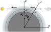 |
Fig. 1 Schematic of the geometry of a light ray crossing the atmosphere. The inner circle is the arbitrary reference surface of the planet of radius Rp. The lighter-grey region is the atmosphere. The distance from the centre of the planet is r = Rp + z. A light ray is defined by its distance of closest approach to the centre of the planet, ρ, and the corresponding tangential altitude zt = ρ − Rp. The direction of the light ray defines the x direction. As we further discuss the extent of the limb along the ray, we introduce xlimb so that the absorption outside the [−xlimb, xlimb] segment is negligible in determining the transit radius, and the corresponding limb opening angle ψ. |
2 Simple estimate of the maximum width of the limb and goals of the study
The day–night transition would not be a problem if the region probed in transmission were infinitely thin. We would just see a slice of the atmosphere. But in fact, and quite counter-intuitively, the width of this region – which is our definition of the limb1 – is much larger on some planets than generally expected. Therefore, the transit spectrum encodes a much wider diversity of temperatures and compositions.
Although the effect of this larger extent of the limb is demonstrated below a posteriori by the results of our 3D transit model, let us here try to give simple arguments to estimate how different planets can be affected. In other words, how wide can we expect the limb to be on any given planet?
Of course, the problem in providing such a simple estimate is that the region that contributes to the transit spectrum does not only depend on the global parameters of the planet, but also on the precise chemical-physical conditions in the atmosphere and how they vary spatially, as is demonstrated below. There is therefore a certain degree of arbitrariness if one wants to come up with a simple general estimate. For this reason, we first use a simple geometrical argument. The advantage of this is that it allows us to identify the key dimensionless parameter controlling the limb width. In Appendix A we derive a model of a more specific case of chemical inhomogeneity and show that the two approaches indeed yield similar results.
Let us consider a light ray passing through the limb as shown in Fig. 1. Estimating the width of the limb comes down to the computation of the maximum distance from the limb plane, xlimb, at which the atmosphere still measurably affects the optical depth along all the observed rays, and especially the deepest one. The choice we have to make here is the highest pressure probed in transit (Pbot, that we assume to define the planetary radius Rp) and the lowest pressure at which the atmosphere is still able to significantly affect the transmission of a given ray (Ptop). Then the width of the limb is given by
 (1)
(1)
Due to the fact that, in an isothermal atmosphere with an atmospheric scale height at the surface equal to H and a varying gravity, the hypsometric relation writes
 (2)
(2)
we get
 (3)
(3)
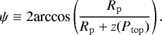
The first important result is that we see that the important dimensionless quantity in our problem is the ratio of the scale height to the planetary radius. The higher this parameter, the larger the curvature effects in the atmosphere. This parameter appears often in the following analyses. We also directly see that the larger the pressure range probed, the wider the limb. Many models predict that the lowest levels probed in transit are around 100 mb in the visible/near infrared. On the other hand, Kreidberg et al. (2014) showed that in order to explain the flat spectrum of GJ 1214 b, an opaque aerosol deck is needed as high as 10−3 –10−2 mb, showing that absorbers at such altitudes can indeed still affect the transit spectrum.
To get a quantitative idea of the possible width of the limb, Fig. 2 shows the result of Eq. (3) as a function of the planetary radius and scale height of the atmosphere. To obtain a relatively conservative estimate, we restrained the pressure range to (Pbot, Ptop) = (10 mb, 10−2 mb). One can see that even for the Earth, the limb region already spans more than ten degrees. For a warm sub-Neptune planet like GJ 1214 b, this can be as large as 45°–50°. In numerical terms, this means that within a 3D atmosphere model of this planet with a typical resolution, say 128 grid points in longitude for sake of concreteness, a single ray would interact with about 24 consecutive horizontal cells before leaving the planet. From these numbers, it becomes evident that the 1+1D approach, by picking only one out of those 24 cells as representative of the terminator, is a crude approximation to a real transmission spectrum.
Our goal is to identify the various biases of retrieval methods created by thermal and compositional – including clouds – inhomogeneities in the atmosphere in transmission. To that purpose, we need a transmission-spectrum generator able to match the complexity of a real 3D planet. We therefore developed a tool able to compute transmission spectra using a parametrized 3D atmospheric structure or the outputs of a 3D atmospheric simulation by a global climate model – namely the LMD Generic model (Wordsworth et al. 2011; Leconte et al. 2013; Charnay et al. 2015). This tool, Pytmosph3R, and its architecture are described in Sect. 3. We then show an extensive validation in Sect. 4. Subsequently, Sect. 5 presents a first application of this tool to a simulation of the atmosphere of GJ 1214 b where we demonstrate the necessity of a real 3D approach to model data for such precise observatories. Finally, we investigate how day–night temperature gradients expected for exoplanets cause a systematic bias in retrieval analysis of real data performed with 1D forward models (Sect. 6).
 |
Fig. 2 Simple estimate of the opening angle of the region around the terminator that affects the transmission spectrum (i.e. the limb). The contours give the opening angle in degrees as a function of the planetary radius and the atmospheric scale height of the atmosphere at 10 mb (the variation of gravity with height is accounted for). The atmosphere is assumed to become transparent above the 1 Pa pressure level. Black dots are known planets for which the radius and surface gravity are measured. Some key objects are identified. The equivalent temperature is derived from the scale height assuming an atmosphere of hydrogen and helium (solar abundances) and a surface gravity of 10 m s−2. For hot, low-gravity planets like GJ 1214 b, the limb can cover almost half the surface of the planet. |
3 Presentation of Pytmosph3R
Pytmosph3R is designed to compute transmission spectra based on 3D atmospheric simulations performed with the LMDZ generic global climate model. It produces transmittance maps of the atmospheric limb at all wavelengths that can then be spatially integrated to yield the transmission spectrum. The code is entirely written in Python. In this section we present the various modules of the code:
-
the geometrical framework used to map the atmospheric structure from the spherical coordinates used by the GCM onto cylindrical coordinates that are more suitable for following photons crossing the atmosphere;
-
the two algorithms that can be used for the calculation of the slant optical path – a discretised and an integral method;
-
the various sources of opacity included in our radiative-transfer model;
-
the spatial integration to produce spectra.
3.1 Definition of coordinate systems
3.1.1 The spherical grid used in atmospheric simulations
Typical 3D atmospheric simulations – LMDZ included – provide state variables such as temperature and mixing ratios of various absorbers/scatterers on a longitude/latitude/pressure grid. Although pressure is a convenient variable to compute atmospheric motions, transit spectroscopy is fundamentally about knowing the physical area of the opaque region of the atmosphere. We must therefore first interpolate the outputs of the climate model on a spherical (λ, φ, z) grid, where λ is the longitude, φ is the latitude, and z the altitude. When needed, we also refer to r ≡ Rp + z, the distance to the planet centre, or α the colatitude.
The longitude/latitude grid is evenly spaced and follows the native grid of the atmospheric model. The altitude grid is also evenly spaced. However, as is discussed in detail in Sect. 4, the resolution of this grid can, and usually should, be higher than the native resolution of the input simulation as it sets the precision of the output spectrum. We find that a good compromise between computation time and accuracy is reached for a vertical resolution of about a tenth of the scale height. We set nz, nλ, and nφ to be the number of grid cells in each of the three dimensions.
The top should also be chosen to be high enough for the atmosphere to be transparent there. This is quantified hereafter. If this altitudeis above the top of the input simulation, the code extrapolates the atmosphere above this top assuming hydrostatic equilibrium and a fixed temperature (or a profile that the user needs to define).
Subsequently, we integrate the hydrostatic equilibrium equation within each column of the model to compute the values of all the necessary variables from the climate model (e.g. temperature and mixing ratios) on this new altitude grid. During this integration, the variation of gravity with altitude is taken into account (see Eq. (7)), an effect that proved to be crucial to reach the precision needed.
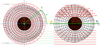 |
Fig. 3 Schematic showing the cylindrical grid (in green). Left panel: grid as seen from the observer. The pink dots are examples of (ρ, θ)-rays (to follow the Python convention used by the code, the indices given start at 0). The native GCM grid at the terminator of an example simulation is shown in black to illustrate its non-uniform vertical spacing. Right panel: the side where we can follow light rays (dashed lines) as they go horizontally from left to right. The red boxes illustrate how the x-discretisation is computedfor each ray to follow closely where it goes from one cell of the spherical grid to another. |
3.1.2 The cylindrical grid used for the radiative transfer
As long as the light from the star propagates in straight lines, cylindrical coordinates provide the most natural set to treat transit geometry. Indeed, due to the great distance between the observer and the planet, light rays follow parallel paths so that the radiative transfer can be solved within a hollow cylinder that is tangent to the planetary surface at the bottom and stops at the top of the modelled atmosphere.
We therefore define a cylindrical grid whose coordinates are denoted (ρ, θ, x) where the x-axis is the line between the centre of the planet and the observer (the line of sight), with x increasing toward the observer (see Fig. 3). The x = 0 plane corresponds to the plane perpendicular to the line of sight passing through the centre of the planet (hereafter referred to as the plane of the sky). The factor ρ is the distance from the x-axis in the plane of the sky, and θ is the azimuth, defined here as the angle on the limb plane measured from a reference direction (see below).
Hereafter, we refer to the ray of light that crosses the limb plane at those coordinates as a “(ρ, θ)-ray”. The transmittance map of the atmosphere is simply constructed by computing the chord optical depth of the ray along the x direction for every (ρ, θ). From this, and assuming a luminosity/spectral distribution (limb-darkening, spots) over the stellar disc as well as a transit trajectory, we can produce spectral transit light curves.
The resolution of the cylindrical grid is based on that of the spherical one, which has a finer altitude resolution compared to the GCM: Δρ = Δz and Δθ = Δφ. There is no benefit in increasing the resolution in θ, GCM cells being considered horizontally uniform. To test the impact of shooting our rays through the middle of our layers or at their interfaces, the ρ grid can be shifted relative to the r grid using the ω parameter (0 ≤ ω < 1) so that ρ = r+ ω Δz. To speed up computation, (ρ, θ)-rays are eventually divided irregularly along the x direction in order to closely follow their path from one spherical cell to another, as explained in Sect. 3.2 (see also Fig. 3).
3.1.3 Orientation of the planet and correspondence between coordinate systems
The cylindrical coordinate system needs to be properly oriented with respect to the spherical grid. For this, we simply require knowledge of the longitude and latitude of the observer in the spherical coordinates, (λobs, φobs), at the timeof observation (or alternatively the colatitude αobs)2. The unit vector pointing toward the observer,  , then defines the direction of the x-axis of our cylindrical coordinates.
The last thing that we need to define is the arbitrary reference direction for the azimuth. For this we choose the projection of the rotation axis of the planet onto the plane of the sky.
With these two definitions, there is a unique relationship between the spherical and cylindrical coordinates for a given point. The translation from one system to the other with an arbitrary orientation however requires a set of non-linear equations to be solved; detailed in Appendix B.
3.2 Dividing (ρ, θ)-rays into subpaths
Along each (ρ, θ)-ray (identified by the indices iρ and iθ) we locate all the intersections with relevant interfaces of the spherical grid and divide the ray into segments of irregular lengths, each of them belonging to a different cell. All quantities used to calculate the optical path – pressure and density excepted – are considered constant within each segment/cell. The pressure/density can be either kept constant within a segment/cell or assumed to follow hydrostatic equilibrium.
In practice we first divide each (ρ, θ)-ray with a constant Δx step, calculate the spherical coordinates of the resulting discrete points and give them the three indices (ir,iλ,iφ) of the spherical cell they belong to (see Appendix B). The step Δx is chosen to be small enough (<Δz) that two successive points can only belong to either the same cell or to two adjacent cells (i.e. cells separated by a facet, an edge, or a corner). One, two, or all three indices (ir,iλ,iφ) can be incremented between two successive points.
When a change of index occurs between two points, the code analytically determines the position of the intersection(s) between the (ρ, θ)-ray and the surface(s) separating cells. This comes down to solving for the unknown position xint along the ray knowing ρ, θ, and the equation of the surface(s) crossed. The equations to be solved for the three types of intersections (depending on the varying index) are detailed in Appendix C.
From these positions, the length of the subpaths belonging to individual cells can be measured. When more than one index is incrementedbetween two points (near an edge or a corner, which implies that a third cell has been crossed) and once the intersectionshave been located, their x-position are sorted in increasing order so that subpaths can be measured and attributed to specific cells.
3.3 Optical depth
At this point, all the (ρ, θ)-rays are now subdivided into Nx(ρ, θ) segments of length  . The number and length of these segments of course changes for each (ρ, θ)-ray depending on the number of intersections found in the previous step. Each of these segments has been assigned to a given cell of the spherical grid so that we know all the quantities describing the physical state of the atmosphere in the ith segment: temperature (Ti), volume mixing ratioof the jth of the Nspe species (χj,i), and the mass mixing ratioof the kth of the Ncon species of condensed particles (qk,i).
The goal is now to compute the optical depth (hence the transmittance) of the atmosphere for each (ρ, θ) which is given by
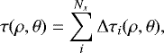 (4)
(4)
where Δτi is the optical depth of a given segment.
Pytmosph3R can calculate optical depth in two ways. Pressure (and density) can be either considered constant within a cell, hereafter referred to as the discretised method, or it can be integrated along the optical path assuming a hydrostatic vertical structure within the cell, the so-called semi-integral method. In both cases, we assume that cross-sections are constant along the given sub-path to spare considerable CPU time. This approximation yields negligible errors as long as the simulation is sufficiently resolved in the vertical.
3.3.1 Discretised calculation of the optical depth
With the discretised method, pressure and density are considered constant so that the optical depth of a segment simply reduces to
 (5)
(5)
where σmol, σsca, and σcon are the cross-sections for the molecular, Rayleigh scattering, and continuum absorptions, respectively, and kmie is the absorption coefficient associated to the Mie scattering by aerosols. The parametrization used for these absorptions is discussed below.
3.3.2 Integral method
With the integral method, we now assume that the pressure follows the hydrostatic law within a segment, thus varying with altitude. The optical depth of a segment for any contribution is then given by
 (6)
(6)
where xi is the position of the beginning of the segment. We use zi to refer to the corresponding altitude. The simplification comes from the fact that the altitude profile of the pressure within an isothermal atmosphere is analytical even if the gravity varies with height. It is given by
 (7)
(7)
where M is the molar mass of the gas, R the universal gas constant, and g(z) the gravity at a given altitude. This entails
![Mathematical equation: \begin{eqnarray*} \int_{\x_{i}}^{\x_{i} +\dxrt_{i}}P(z(x)) \,\mathrm{d} x &=& \int_{\x_{i}}^{\x_{i} +\dxrt_{i}}P(z_1)\exp\left[-\frac{M g(z_{i})}{R T_i}\!\left(\frac{z-z_{i}}{1+\frac{z-z_{i}}{R_{\mathrm{p}}+z_{i}}}\right)\right]\mathrm{d} x \nonumber\\ &=& \int_{z_{i}}^{z_{i} +\Delta z_{i}}P(z_{i})\exp\left[-\frac{M g(z_{i})}{R T_i}\left(\frac{z-z_{i}}{1+\frac{z-z_{i}}{R_{\mathrm{p}}+z_{i}}}\right)\right]\nonumber\\ &&\times\frac{(R_{\mathrm{p}}+z)}{\sqrt{(R_{\mathrm{p}}+z)^2-\rho^2}}\,\mathrm{d} z, \end{eqnarray*}](/articles/aa/full_html/2019/03/aa34384-18/aa34384-18-eq10.png) (8)
(8)
where the last integration is carried out numerically between the lowest and the highest point of the segment. The increased accuracy of this method is due to two factors: (i) the variation of gravity with height is built in, and (ii) more importantly the exponential variation of pressure is fully accounted for. This explains why a much lower number of vertical layers are needed with this method to reach numerical convergence.
3.4 Sources of opacity
3.4.1 Molecular lines
Pytmosph3R deals with molecular absorptions in two possible ways: tables of monochromatic cross-sections or correlated-k coefficients (also called the k-distribution method; Fu & Liou 1992).
Using k-distributions considerably reduces the computing time but new k-tables must be pre-computed each time one wants to change the atmospheric composition or the resolution of the output spectrum.
Because our code is designed to work with the TauREx retrieval code (Waldmann et al. 2015), we use the same set of high-resolution cross-sections produced by the ExoMol project. This data set is precomputed on a T − logP grid going from 200 to 2800 K every 100 K and from 10−3 to 10 bar every 0.3 dex. Pythmosph3R users can either choose linear or optimal interpolation in temperature. For the optimal interpolation we follow Hill et al. (2013) who prescribes
 (9)
(9)
where i is the molecular/atomic species index, λ the wavelength, and T the temperatureof the cell. The (a, b) scaling factors are given by
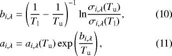
where Tu and Tl are upper and lower temperatures, respectively. k-distributions can only be interpolated linearly in temperature. Along the pressure coordinate, the interpolation is log-linear.
The effect of using different interpolation schemes has been tested and we find that it does not introduce significant differences.
3.4.2 Continuum absorptions
Our principal source of continuum opacity is due to collision-induced absorptions. We account for this process for all the species for which such information is available in the HITRAN database and following the prescriptions of Richard et al. (2012). Furthermore, for specific species such as water vapor, we can add a continuum that accounts for the truncation of the far wings of the lines and the neglect of many weak lines in some of our sets of cross-sections or correlated-k tables. In such cases, the water continuum is added using the CKD model (Clough et al. 1989). We however note that care must be taken to ensure that the molecular opacities used must be computed consistently so as not to count some effects twice.
3.4.3 Rayleigh scattering
Multiple scattering is neglected. The contribution of Rayleigh scattering is therefore treated as a simple extinction. The cross-section of any single gas molecule is given by the common formula
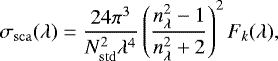 (12)
(12)
where λ is the wavelength (here in m), Nstd is the number density of a gas under standard conditions, nλ is wavelength-dependent, real refractive index of the gas, and Fk(λ) is the King correction factor which accounts for the depolarization. The accuracy of this essential part of the radiative transfer mainly depends on the calculation of refraction indices. We used the most recent data available in the literature. For sake of completeness, we have reviewed the parametrization that we use for H2, He, H2 O, N2, CO, CO2, CH4, O2, and Ar in Appendix D and in Table D.1.
3.4.4 Mie scattering for aerosols
Transmission spectra of transiting exoplanets are affected by clouds and hazes. The LMDZ GCM can include cloud physics and provide the properties and 3D distribution of liquid/solid condensates and aerosols. Assuming spherical particles with a size similar to or larger than the considered wavelengths, we use Mie scattering formalism to compute their extinction factor Qext and resulting opacities, following the same method as in radiative-transfer modules of the GCM (Madeleine et al. 2011). We linearly interpolate the value Qext on effective radius and wavelength using pre-calculated lookup tables. The absorption coefficient is estimated as
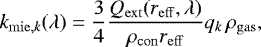 (13)
(13)
where Qext is the extinction coefficient for the wavelength λ and a given effective radius reff, qk and ρcon are the mass mixing ratio and the density of the species considered, respectively, and ρgas is the total gas density.
3.5 Generation of transmittance maps and spectra
To generate the global absorption spectrum of the planet, the wavelength-dependent (ρ, θ) map of optical depth is first converted into a transmittance map
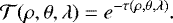 (14)
(14)
In the most general case, the in-transit flux should be computed by convolving this transmittance map with a given surface-brightness distribution for the star. However, in the most simple case of a homogeneous stellar disc, the effective area of the planet reads
 (15)
(15)
where Rp is the radius of the planet (at the bottom of our model atmosphere), Sρ = 2π(ρ + Δρ∕2)Δρ∕Nθ, Nθ being the number of θ points, and Δρ is the layer thickness. Eventually, the relative dimming of the stellar flux due to the planet is given by
 (16)
(16)
where R⋆ is the stellar radius. For each monochromatic transit depth, we can determine an effective radius of the planet defined as
 (17)
(17)
One can simulate a realistic light curve by precisely locating the planet transmittance map over the weighted stellar disc at each time-step of the transit. During ingress and egress, where the stellar disc is hidden by only a fraction of the planet, only the elements in front of the stellar surface need to be considered. Astrophysical (stellar) noise can then be added by simulating a realistic spatial distribution of the star luminosity and its variability during a transit, for example by taking into account limb darkening, spots, and granulation (Chiavassa et al. 2017). This model complements other codes able to produce synthetic emission/reflection spectra and light curves from GCM simulations (Selsis et al. 2011; Turbet et al. 2016, 2018).
4 Model validation
4.1 Validation approach
In the following subsections we validate the different modules of the code: calculation of the vertical structure, 3D geometry of the radiative transfer, integration scheme for the optical depth, interpolation scheme for the opacities, and so on. In the absence of another validated code able to produce synthetic transmission spectra from 3D simulations, we decided to compare our code with a hierarchy of 1D models with increasing complexity – from a purely analytical model (Sect. 4.2) to the more realistic forward spectrum generator used in the TauREx retrieval tool (Waldmann et al. 2015; Sect. 4.3).
In each case, the comparison with a given 1D model proceeds as follows: on one hand we generate a spectrum from the 1D model with a given vertical temperature profile (possibly isothermal). On the other hand, we use the same vertical profile to generate a full spherically symmetric 3D structure on our spherical grid. This structure goes through our whole code to generate a spectrum that should ideally be the same as the 1D spectrum. Finally, we increase the resolution of our 1D/3D grids until convergence is reached.
Relatively early in our tests, it appeared that, to numerical precision, our transmittance maps were completely insensitive to the azimuth angle, θ, in any spherically symmetric configuration, as it should be. This not completely trivial result shows that our careful way of computing the path length of the ray in each cell indeed prevents singularities – in particular at the poles – in our initial longitude/latitude grid. This also allowed us to test the convergence of the algorithm of vertical integration at very high resolutions. Indeed, when a very large number of layers is used – above ~1000, which is already much larger than what is needed in practice for convergence – the computing time for the full 3D code becomes prohibitive. For this reason, in some cases below, the results shown are derived from a sector of the limb only (i.e. a given θ). This approach is made possible by the fact that the numerical differences between the various sectors is negligible.
As expected from our analytical arguments and further demonstrated in the following sections, we find that the most, and in fact almost only, important parameter determining the resolution needed to model a given atmosphere is the ratio of the planetary radius to the scale height (Rp∕H): the lower this parameter, the larger the vertical resolution needed. This stems from two factors. A lower ratio means that (i) gravity will vary more significantly in each vertical layer, and (ii) curvature effects will be more pronounced and rays will pass through more atmospheric columns along their path (see Fig. 2). As a result the validation cases we present hereafter focus on covering a wide variety of Rp ∕H. However, because the scale height is not set, but is determined from the composition and temperature of the atmosphere and from the surface gravity, fixing Rp∕H entails varying one of these parameters to compensate. For each of the validation setups described in the following sections, the compensation parameter is therefore always stated. This can sometimes result in a physically inconsistent set of planetary parameters that we deem acceptable in the context of our validation. The values used for the other parameters are given in Table 1, unless otherwise stated.
As becomes clear in the following, our 3D model can reproduce our validation cases to numerical precision. We used these tests to further derive some guidelines on the number of layers and the model roof pressure to use in various cases to reach a satisfactory accuracy. To quantify what we call a “satisfactory accuracy”, we use the difference on the predicted transit depth between two models and ask that it be significantly smaller than the photon noise that can be expected for the given target in one transit. If one wants a more stringent condition, one can use the expected systematic noise floor for a given instrument (expected to be on the order of a few parts per million with JWST, for example).
Numerical values for the parameters used in our fiducial validation case.
4.2 Validation with a monochromatic analytical model at constant gravity
To focus on the basics of radiative transfer we first compare the optical depths computed with our model with those given by an analytical solution. For an isothermal, horizontally uniform atmosphere with constant gravity and a scale height H ≪ Rp, Guillot (2010) provides an analytical formula for the transmission optical depth as a function of the distance to the centre of the planet:
 (18)
(18)
where τtr is the chord optical depth and τ⊥ the vertical optical depth. As described in Appendix A, we use this formula to calculate the planet transit. We then compare theresults with those of Pytmosph3R for a wide range of vertical resolutions: 50 to more than 10 000 levels. For 1000 levels and more, and as long as the thin atmosphere assumption is respected, the effective absorption radii from both models agree within ~ 1 cm (i.e. ~ 10−9 relative accuracy).
4.3 Comparison to the TauREx forward model
4.3.1 Reasons for benchmarking against the forward model of an atmospheric retrieval tool
As one of our main goals is to perform a retrieval on a spectrum derived from a 3D model as if it were from a real planet, we decided to use the forward model of an existing, and validated, atmospheric retrieval code for our comparison.
The added benefit of this validation approach is that we make sure that in the relevant case of spherically symmetric atmosphere, both our 1D and 3D forward models can produce spectra without any numerical biases – meaning here that the differences between the spectra can always be reduced to be much smaller than the noise that will be prescribed in the retrieval step by choosing a sufficient vertical resolution.
As a result, we know that when we retrieve the properties of an atmosphere generated with our 3D model, the various potential biases in the retrieved parameters are entirely due to the heterogeneities of the atmosphere and not the differences in the numerics.
In our case, we are using TauREx, whose forward model is described in more detail in Waldmann et al. (2015). For the reasons mentioned above, we decided to use the same philosophy used in TauREx in the implementation of many physical processes, in particular concerning the molecular opacities and the Rayleigh scattering. Two notable exceptions are (i) the vertical grid and (ii) the optical path calculations that are discussed in greater detail in thefollowing section. Let us just mention here that our requirement that our 3D model be as compatible with TauREx as possible is the reason for keeping two algorithms for the calculations of the optical depth in the code: the integral scheme which is the optimal scheme in terms of convergence and should be used in general, and the discretised one that always gives a result closer to TauREx when the same number of layers is used in both models.
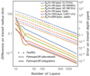 |
Fig. 4 Absolute difference between the transit radius computed for a given number of layers and model and our reference case (integral method, isothermal, grey opacity, 50 000 layers). The dots show the results of TauREx, the dashed lines represent Pytmosph3R in its discretised version, and the solid lines are for the integral version. Results are plotted for six values of Rp ∕H that increase from top to bottom for each set of curves. The names of planets representative of these values are labelled. For Pytmosph3R, we use the results of one sector only (θ = 0°) to keep the computing time reasonable for the most resolved simulations. The axis on the right converts this radius difference into a transit depth difference in the case of GJ 1214 b (i.e. a planet of 2.6 earth radii in front of a star of 0.2 solar radii). To rescale this for any type of planet or star, we multiply by |
4.3.2 Validation for an isothermal, grey atmosphere with varying gravity
We now assume an isothermal atmosphere with an altitude-dependent gravity. We consider a uniform composition of H2 /He/H2O. In this first step, to validate only the geometrical part of the code, we assume that H2 and He are transparent, and that water has a grey opacity that is independent of temperature and pressure. In this set of simulations, the scale height is set to the prescribed value by adjusting the temperature of the atmosphere, all other parameters being kept fixed to the value given in Table 1.
For each Rp∕H ratio, we first compute the transit radius of a high-resolution reference model using Pytmosph3R with 50 000 layers. We then compute the difference between this reference and the transit radius given by our three models at various vertical resolutions. This is summarised in Fig. 4 where the results for the Pytmosph3R/discretised method are shown using dashed lines, for the Pytmosph3R/integral method using solid lines, and TauREx using dots. The various colours are for different Rp ∕H. We note that although we quote some planet names for each ratio to give an idea of what type of planet it describes, all calculations were performed for the same planetary radius (1 RJ).
The conclusions that can be drawn from this test are the following:
-
all three models converge toward the same result as vertical resolution is increased so that the differences can be reduced to an arbitrarily low value;
-
as advertised, atmospheres with a low Rp∕H require less vertical layers to reach a given accuracy;
-
for the same number of layers, the accuracy of our integral version of the code is orders of magnitude better than the discretised one. This is thus the preferred mode for most applications;
-
as expected, the discretised mode, although less accurate, is always closer to TauREx and should probably be used if a retrieval analysis is to be performed. This indeed introduces as little bias as possible during the retrieval step.
In terms of the number of layers needed to reach convergence – the precision needed depends of course on the observations – the integral mode of Pytmoshp3R requires as little as 20–30 layers in almost all practical cases of interest. This yields about two to three points per pressure decade or about one per scale height. For the discretised version as well as for TauREx and indeed most forward models using the same philosophy, 100 layers are generally enough, but this should be taken with caution. Hot and low-gravity objects in particular require a finer resolution and some published models have probably reached convergence only marginally.
Despite our efforts, it can be seen that for a given number of layers, the discrete version of Pytmosph3R is not exactly equivalent to TauREx. We find that this small discrepancy is fundamentally due the fact that our vertical grid uses altitude rather than pressure levels as is usually the case in 1D models. When gravity varies with altitude, an iso-altitude grid is not equivalent to an iso-log pressure grid, hence the small difference.
4.3.3 Comparison with the full TauREx forward model
Here we compare spectra from Pytmosph3R and TauREx for isothermal atmospheres with the same composition as before. There are two differences however. First, we now compute a full spectrum with all our opacity sources varying with wavelength, temperature, and pressure. Second, we now fix the atmosphere temperature beforehand and adapt the surface gravity of the planet to get the desired Rp ∕H ratio. This stems from the fact that temperature will now impact the molecular features directly and not only through the scale height. This allows us to test our interpolations in the opacity databases as well.
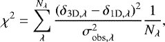
As the model produces a full spectrum and not only a monochromatic transit radius, we quantify the differences between the two codes using a reduced chi-square calculated as follows:
 (19)
(19)
where δ3D,λ and δ1D,λ are the transit depths at the wavelength λ given by Pythmosph3R and TauREx, Nλ is the number of spectral bins, and σhν,λ is the stellar photon noise computed for JWST observations. The latter is given by
 (20)
(20)
where
 (21)
(21)
Here, τλ is the system throughput, R* and Ts are the radius and temperature of the host star, respectively, A is the collecting area of the telescope (here 25 m2), Δt is the integration time, and d is the distance of the target. In our example, we considered a Sun-like star, a one-hour integration, and a system at 100 ly. Increasing the noise tends towards making Pytmosph3R and TauREx spectra indistinguishable.
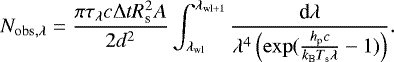
We computed the logarithm of this reduced chi-squared as a function of the atmospheric temperature and Rp ∕H for four different vertical resolutions. Results are shown in Fig. 5.
As already discussed, we can see that the agreement between the two codes at a given vertical resolution generally increases with Rp ∕H. At a given Rp∕H ratio and in this specific example, the agreement also slightly depends on temperature. This is due to the overall increase of H2 O opacity withtemperature that pushes the opaque region upward and increases the limb opening angle (see Fig. 2). With high enough vertical resolution the two models can however agree well within the noise budget. As the lowest encountered Rp ∕H is about 100 (for a hot-Neptune like GJ 1214 b), we confirm that 50 layers should be sufficient in most cases. These maps can however be used as a guide to chose the resolution needed if a more stringent case is found.
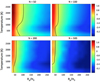 |
Fig. 5 Decimal logarithm of the reduced chi-square for the effective radius between our 3D model and the full forward model from TauREx over a range of temperature between 200 and 2600 K and of Rp∕H between 40 and 260. As a comparison, all planets described in Fig. 4 have Rp∕H > 100. The black line shows where the reduced χ2 equals unity, i.e. where model differences become insignificant compared to the noise. We assumed an error calculated with a sun-like star at 100 lyr, 1 h of integration and JWST instruments. The same work has been done for four vertical resolutions: 50, 100, 200 and 500 layers. |
4.4 Effect of model top altitude
When computing transmission spectra, if the model does not reach a height in the atmosphere that is transparent enough at all wavelengths, the transit radius of the planet may be underestimated in opaque parts of the spectrum. The choice of the model top pressure therefore generally results from a trade-off between computation time and convergence.
This point is even more crucial here because several other technical reasons can limit the maximum altitude of a 3D climate model to a few tenths of a pascal or more (short radiative timescales, absence of non-LTE radiative treatment or conductive heat transfer, etc.).
To illustrate these limitations, Fig. 6 shows two spectra computed by Pytmosph3R for a simulation of GJ 1214 b (see Sect. 5). The black spectrum directly uses the outputs of the global climate model and stops around a pressure level of 0.5 Pa. The blue spectrum is obtained by extending the model upward to 10−4 Pa assuming that the atmosphere remains isothermal above the GCM model top. For this particular case, this is necessary and sufficient to reach a degree of convergence commensurate with the future precision of the data (~ 1−10 ppm). Extending the model to even lower pressures does not significantly change the resulting spectrum.
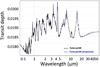 |
Fig. 6 Transit spectrum generated by Pytmosph3R from the outputs of a GCM simulation of GJ 1214 b (Charnay et al. 2015). The black curve represents the effective radius obtained when accounting only for the part of the atmosphere explicitly modelled by the GCM (down to ~ 0.5 Pa). The blue curve shows the result when the model is extended by an isothermal atmosphere down to 10−4 Pa. Further lowering the pressure of the model top does not alter the spectrum. |
5 The case of GJ 1214b as an illustration of Pythmosph3R capabilities
In this section, we apply Pythmosph3R to GCM simulations of the atmosphere of GJ 1214 b to illustrate the possibilities of the code. This also allows us to show examples of horizontal inhomogeneities and some of their effects on transmission spectra. Despite the flat spectra currently obtained with WFC3/HST, possibly due to high-altitude clouds/aerosols (Kreidberg et al. 2014), GJ 1214 b is one of the rare known targets that is not a gas giant but still offers a favourable configuration for transmission spectroscopy: the vicinity to the Sun (13 pc), a low-density implying the presence of an atmosphere, a short period (1.58 d), a red dwarf host, and an expectedly high scale-height-to-radius ratio (see Fig. 2). Modelling the formation, distribution and spectral signature of aerosols motivated the use of a 3D atmosphericmodel of the atmosphere (Charnay et al. 2015) to compute transmission maps and spectra with Pythmosph3R.
5.1 Input 3D atmospheric model
We use the “100× solar metallicity” simulation of Charnay et al. (2015) made with the LMDZ generic global climate model. The simulation has a 64 × 48 horizontal resolution with 50 layers equally spaced in log pressure, spanning 80 bars to ~ 0.5 Pa. An important assumption in this simulation is the local chemical equilibrium: in each cell, the composition is imposed by the local temperature, pressure, and elemental composition. As the simulation assumes a circular orbit with null obliquity and a synchronized rotation, the state of the atmosphere after convergence is relatively stable, exhibiting only stochastic variations. We use an arbitrary time-step to produce synthetic spectra. The thermal structure is shown in Fig. 7 and the absorber/cloud distribution in Fig. 8. We redirect the reader to Charnay et al. (2015) for more details on the model.
 |
Fig. 7 Colour maps showing the temperature distribution in the model atmosphere of the 100× solar metallicity simulation from Charnay et al. (2015). The inner white disc represents the inner part of the planet with a radius assumed to be equal to that of GJ 1214 b (17.600 km). Top panel: temperature at the terminator. The planet is seen from the observer during transit, the poles being at the top and bottom. Bottom panel: the star is on the left and the observer on the right on the z = 0 axis. The poles are on the x = 0 axis. From centre outward, the five solid lines are respectively the 106, 103, 1, 10−2, and 10−4 Pa pressure levels. The outer circle is there as an eye guide to highlight the non-sphericity of the planet. Temperature is well homogenised below the ~103 Pa level. Maps are to scale and show that the dayside is noticeably more vertically extended than the nightside. |
5.2 Transmittance maps
In order to understand the global transmission spectrum Pythmosph3R offers the possibility to draw a transmittance map in any spectral bin of the spectrum. Viewing the azimuthal and vertical inhomogeneities provides some important information for the interpretation of spectral features.
Figure 10 shows transmittance maps for a simulated atmosphere of GJ 1214 b, with and without the effect of clouds. Temperature is directly or indirectly at the origin of the inhomogeneities. Colder regions at the western terminator are less extended vertically, and locally induce a smaller absorption radius. As the simulation imposes a local chemical equilibrium, colder regions are also poorer in CO2 and richer in CH4, affecting the transmittance distribution in the displayed CO2 (14.9 and 4.3 μm) and CH4 (1.17 μm) bands. In the 14.9 μm CO2 bands another thermal effect comes from the strong temperature dependency of the absorption cross-section, which strongly enhances the transmittance inhomogeneities compared with the 4.3 μm band, and is much less sensitive to temperature. The effect of clouds is the strongest at 0.95 μm although they mask some chemical inhomogeneities at high pressure.
 |
Fig. 8 Distribution of the logarithm of the mass mixing ratio of some absorbing species at the terminator in a simulation of the atmosphere of GJ 1214 b by Charnay et al. (2015). For KCl and ZnS, only the molecules in the condensed phase are considered. The dashed (solid) black curves are the contour of unit optical depth with (without) cloud opacities at a wavelength relevant to the molecule considered (1.17 μm for CH4; 4.30 μm for CO2; 1.08 μm for KCl et ZnS). The size of the inner white disc delimiting the base of the atmosphere is reduced for clarity. The whole simulated atmosphere is shown. The two white circles delimit the region enlarged in Fig. 10. |
 |
Fig. 9 Decimal logarithm of the column density of some molecules in the star-observer direction for a simulation of the atmosphere of GJ 1214 b by Charnay et al. (2015). See the caption of Fig. 8 for details and notations. |
5.3 Comparison with averaging methods based on 1D models
In the absence of a code like Pythmosph3R, producing a transmission spectrum from a 3D simulation using a radiative-transfer model based on a horizontally homogeneous atmospheric profile implies an average of some kind.
5.3.1 Mean profile
One method consists in averaging first the atmospheric quantities and then computing a transmission spectrum. One single atmosphericprofile (temperature, pressure, chemical abundances and cloud properties as a function of altitude) is obtained by averaging the 2N − 2 profiles found on the terminator, weighted by the fraction of azimuth covered by each cell (N being the number of latitude points on the simulation grid). The transmission spectrum is then computed assuming that this atmosphericprofile covers the whole planet. Figure 11 shows the comparison between spectra resulting from this mean profilemethod and those generated by Pytmosph3R.
The difference is mostly due to the lower-temperature patch at the morning terminator near the equator (west of the substellar point) which is due to the equatorial jet bringing cold air from the nightside there (see Fig. 7). This difference is considerably larger than the expected photon noise with JWST over most of the spectrum making this method clearly inadequate. This, in a sense, already highlights why 1D retrieval methods may be biased when interpreting the spectra of real atmospheres.
5.3.2 Limb integration
A better technique that is often applied (e.g. by Charnay et al. 2015; Way et al. 2017; Parmentier et al. 2018; Lines et al. 2018), involves computing in a first step 2N − 2 transmission spectra assuming a horizontally homogeneous atmosphere, one for each atmospheric column found on the terminator. The total transmission spectrum is then calculated as an average of these intermediate spectra, weighted by the fraction of azimuth covered by each column. Figure 12 compares spectra obtained with this limb integration technique and shows the comparison between spectra resulting from this approach (red line) and from Pytmosph3R (red line).
A quick comparison of Figs. 11 and 12 clearly shows that limb integration performs much better than the mean profile approach. However, significant discrepancies remain throughout the spectrum and especially in some molecular bands. By definition, these differences only come from the atmospheric inhomogeneities along the path of the ray. These are due to the effect of the following factors.
-
Day–night temperature gradient: as the dayside is hotter than the night side, the vertical extent of the atmosphere changes along the ray. As shown in Sect. 6, this causes a net increase in absorption visible in the water bands (see lower panels of Fig. 12). Although this effect is on the order of the photon noise for a single transit for the (relatively) cold atmosphere of G J1214 b, it can strongly affect the retrieval of the properties of hotter planets as demonstrated in the following section.
-
Day–night compositional gradient: for the absorption bands due to absorbers with a heterogeneous distribution (like CO2 in our case, which absorbs prominently at 4.5 and 15 μm) a change of composition along the line of sight creates a signal that is much greater than the expected noise and that cannot be modelled by the limb integration method. Below, we discuss the possible causes of such a compositional gradient. Although it is the most prominent effect in our GJ 1214 b model, the parameter space to be covered in order to fully quantify it is large and is deferred to a future study.
-
Day–night asymmetry of the cloud distribution: the temperature change at the terminator, in turn, allows us to expect changes in the properties of the clouds there (Lee et al. 2016). This will also be looked at in a future study.
 |
Fig. 10 Transmittance maps obtained with the simulation of the atmosphere of GJ 1214 b depicted in Fig. 8. The region shown between the inner white disc and the outer black dotted circle is an enlargement of the region delimited bywhite circles in Fig. 8. The white dotted circle corresponds to the effective radius: the radius of the opaque disc resulting in the same overall absorption as the simulation over a homogeneous stellar disc. The maps in the upperrow are obtained with Mie scattering turned off in order to show the effect of clouds. Clouds dominate near 0.95 μm, methane is the main gaseous absorber at 1.17 μm, and carbon dioxide at 4.30 μm. |
5.4 Comments on the possible causes of compositional heterogeneities
In the model of GJ 1214 b we use, the concentrations of CO, CO2, and CH4 are computed assuming chemical equilibrium. For such atmospheres and cooler ones, the 3D variations of these species are therefore strongly overestimated. While the hottest regions of the atmosphere (above ~ 1000 K) are expected to reach equilibrium faster than typical dynamic timescales, this is not the case in the coldest layers (below ~ 700 K) probed by transmission, where endothermic reaction becomes extremely slow. As a consequence, thermochemistry is expected to produce a more homogeneous composition controlled by the hottest and deepest regions.
However, more irradiated planets must have hotter atmospheres overall, spanning a larger range of temperatures (due to shorter radiative timescales) with very different equilibrium compositions and kinetics fast enough to maintain local equilibrium (Agúndez et al. 2014). These atmospheres are expected to exhibit the strongest horizontal variations of temperature and composition. Parmentier et al. (2018) recently showed that water itself may be dissociated on the dayside of some hot Jupiters and recombine close to their terminator. In addition, UV-driven photochemistry may create additional heterogeneities by allowing some reactions to take place on the dayside of the planet only.
We can thus expect hot planets to exhibit strong day–night compositional gradients that may become a dominant issue in retrieving atmospheric properties through transmission spectroscopy. Quantifying the stellar irradiation at which these effects become significant will require further modelling.
 |
Fig. 11 Transit spectra computed from a 3D simulation of GJ 1214 b atmosphere by Charnay et al. (2015) with Pythmosph3R (black) and a mean profile approximation (see text). Spectra are shown with (right panels) and without (left panels) the radiative effects from the KCl and ZnS clouds. In both cases the atmosphere is extrapolated vertically beyond the top of the simulation. Cloud particle radius is fixed to 0.5 μm. The plots on the lower part show the difference between the two methods. The purple line indicates the photon noise with a JWST aperture, an exposure time of twice the transit duration and a (low) resolution of R = 100. |
6 Effect of dayside–nightside temperature differences on retrieval
As visible in Fig. 2, the region probed in primary transit is much larger than is usually acknowledged, especially on hot and/or low-gravity objects. Therefore, during transit, we are not only probing a thin plane – the so-called terminator – but an area thatcan extend significantly on both the day and night sides. Because these two parts of the planets are expected to exhibit quite different temperatures (as visible in Fig. 7), it seems important to quantify the extent of the imprint of this temperature inhomogeneity on the transit spectrum of the planet, and how it will affect any attempt to retrieve the temperatureat the terminator.
To answer these questions, we conduct a simple experiment. For two prototypical planets (based on GJ 1214 b and HD 209458 b), we build idealised 3D atmospheric structures that are symmetric about the star–planet axis but that continuously go from a high temperature Tday on the dayside to a lower temperature, Tnight, on the nightside. The atmosphere is assumed to have a uniform composition to enable us to concentrate on thermal effects. We then simulate the transit spectrum and try to invert it. Finally, the retrieved temperature is compared to the input one.
6.1 Parametrization of the atmospheric structure
The structure that we chose for the atmosphere is inspired by the 3D simulations of Charnay et al. (2015) for GJ 1214 b whose temperature distribution is shown in Fig. 7. Its most salient feature is the continuous transition in temperature between the day and night sides. For simplicity, we assume that this transition occurs linearly over a region that is parametrized by its opening angle – hereafter referred to as the transition angle (β).
Moreover, as is well known and further exemplified by Fig. 7, the atmosphere of gaseous exoplanets is usually well mixed at depth. The temperature is therefore assumed to be uniform below a pressure level Piso (taken to be10 mb as in the simulation, although some models predict inhomogeneities to persist at deeper levels).
In summary, for a given location identified by its pressure, P, and the (possibly negative) local solar elevation angle, α⋆, the temperature is given by
 (22)
(22)
Examples of such idealized atmospheric structures are shown in Fig. 13 for three different day-night transition angles. We chose to show the structures that are most representative of the real GJ 1214 b case to allow for a direct comparison with Fig. 7. For brevity we also refer hereafter to the “uniform case”: this refers to a case where the whole upper atmosphere has a uniform temperature equal to that at the terminator that serves as a comparison. Therefore, in this case,
 (23)
(23)
Once our four parameters – Tday, Tnight, β, and Piso – have been chosen, the 3D atmospheric structure is integrated from the surface of the planet that is assumed to be the 10 bar level. Hereafter, we refer to the radius of this isobar as Rp, and assume that it contains most of the mass of the object, meaning that the gravity above this level only depends on the altitude.
The reason we are performing such a test on idealised structures and not more realistic ones from a GCM is that we want to isolate the effect of the day–night heterogeneities. In a GCM simulation, there would also be vertical and equator–pole temperaturevariations that would preclude the identification of a single effect.
 |
Fig. 12 As in Fig. 11 but the Pythmosph3R spectra (black) are compared here with those obtained with the limb integration approximation (red). |
 |
Fig. 13 Colour maps showing the temperature distribution of our model atmospheres in a plane perpendicular to the terminator for three different transition angles between a 650 K dayside and a 300 K nightside (from left to right, the day–night transition angle is β = 15, 30, and 60°). The inner white circle represents the inner part of the planet with a radius assumed to be equal to that of GJ 1214 b (17.600 km). The star is on the left and the observer on the right on the y = 0 line. From the centre outward, the five solid lines are respectively the 106, 103, 1, 10−2, and 10−4 Pa pressure levels. Below the 103 Pa level, the atmosphere is assumed to efficiently redistribute heat and is horizontally isothermal. These maps are to scale and show that the dayside is noticeably more extended than the nightside. |
6.2 Effect of the day–night temperature difference on the transmission spectrum
One might naively expect that because of the symmetry of our temperature distribution, the contributions of the hot and cold sides should cancel out. This is however not the case, as can be seen in Fig. 14.
Indeed, by comparing the transmittance map for a given planet in a uniform case, or with a day–night temperature gradient, we directly see that the opaque region extends higher up in the latter case. The greater scale height on the dayside is not compensated by the lower one on the night side.
This can be understood easily using a slightly modified version of the analytical model of Guillot (2010) or Vahidinia et al. (2014) where we separate the atmosphere into two hemispheres that differ only through their temperatures – and thus atmospheric scale heights (Hday and Hnight) – above the pressure level Piso which is located at an altitude ziso above the reference radius of theplanet Rp. Below ziso, the scale height is the same everywhere (Hiso). In essence, this corresponds to the case described above in the limit where β → 0.
We follow the notations in Fig. 1 and the formalism in Appendix A. The difference here is that the scale-height variations mean that the number density at a given altitude is
![Mathematical equation: \begin{align*} n(z)=\left\{\begin{array}{ll} \!\!\!\!\ngas_0 e^{-\frac{z}{\H_{\mathrm{iso}}}} & z < z_{\mathrm{iso}}\\[4pt] \!\!\!\!\ngas_0 e^{-\frac{z_{\mathrm{iso}}}{\H_{\mathrm{iso}}}}e^{-\frac{z-z_{\mathrm{iso}}}{H_{\mathrm{i}}}} &z > z_{\mathrm{iso}} \end{array}\right.\!\!\!, \end{align*}](/articles/aa/full_html/2019/03/aa34384-18/aa34384-18-eq25.png) (24)
(24)
where i is either day or night depending on the hemisphere.
In the limit where all the altitudes in the atmosphere are small compared to Rp, the slant optical depth is the sum of the dayside and nightside contributions, yielding
![Mathematical equation: \begin{align*} \hspace*{-2pt}\left. \tau_{\mathrm{tr}} \right|_{\z_{\mathrm{t}}>z_{\mathrm{iso}}}&=\overbrace{\int_{-\infty}^0 n \sigma_{\mathrm{mol}} \mathrm{d} x }^{\mathrm{day}} +\overbrace{\int_0^{\infty} n \sigma_{\mathrm{mol}} \mathrm{d} x}^{\mathrm{night}}\nonumber\\[4pt] &= \sigma_{\mathrm{mol}} \ngas_0 e^{-\frac{z_{\mathrm{iso}}}{\H_{\mathrm{iso}}}} \left(\sum_{\mathrm{i=day}}^{\mathrm{night}}e^{-\frac{\z_{\mathrm{t}}-z_{\mathrm{iso}}}{H_{\mathrm{i}}}}\int_0^{\infty} e^{-\frac{x^2}{2 R_{\mathrm{p}} H_{\mathrm{i}}}}\mathrm{d} x \right) \nonumber\\[4pt] &=\sigma_{\mathrm{mol}} \ngas_0 e^{-\frac{z_{\mathrm{iso}}}{\H_{\mathrm{iso}}}} \left(\! e^{-\frac{\z_{\mathrm{t}}-z_{\mathrm{iso}}}{\H_{\mathrm{day}}}}\!\!\!\!\sqrt\!{\frac{\pi R_{\mathrm{p}} \H_{\mathrm{day}}}{2}} + e^{-\frac{\z_{\mathrm{t}}-z_{\mathrm{iso}}}{\H_{\mathrm{night}}}}\sqrt{\frac{\pi R_{\mathrm{p}} \H_{\mathrm{night}}}{2}} \!\right), \end{align*}](/articles/aa/full_html/2019/03/aa34384-18/aa34384-18-eq26.png) (25)
(25)
if zt> ziso, and
![Mathematical equation: \begin{align*} \hspace*{-2pt}\left. \tau_{\mathrm{tr}} \right|_{\z_{\mathrm{t}}<z_{\mathrm{iso}}} =&\;\sigma_{\mathrm{mol}} \ngas_0 \left(\int_{-\sqrt{2(z_{\mathrm{iso}}-\z_{\mathrm{t}})R_{\mathrm{p}}}}^{\sqrt{2(z_{\mathrm{iso}}-\z_{\mathrm{t}})R_{\mathrm{p}}}} e^{-\frac{\z_{\mathrm{t}}}{\H_{\mathrm{iso}}}}e^{-\frac{x^2}{2 R_{\mathrm{p}} \H_{\mathrm{iso}}}}\mathrm{d} x \right. \nonumber\\[4pt] &\left. +\,e^{-\frac{z_{\mathrm{iso}}}{\H_{\mathrm{iso}}}}\sum_{\mathrm{i=day}}^{\mathrm{night}}\int_{\sqrt{2(z_{\mathrm{iso}}-\z_{\mathrm{t}})R_{\mathrm{p}}}}^{\infty} e^{-\frac{\z_{\mathrm{t}}-z_{\mathrm{iso}}}{\H_{\mathrm{i}}}}e^{-\frac{x^2}{2 R_{\mathrm{p}} \H_{\mathrm{i}}}}\mathrm{d} x\right)\nonumber \end{align*}](/articles/aa/full_html/2019/03/aa34384-18/aa34384-18-eq27.png)
![Mathematical equation: \begin{align*} =&\;\sigma_{\mathrm{mol}} \ngas_0 \left(e^{-\frac{\z_{\mathrm{t}}}{\H_{\mathrm{iso}}}}\sqrt{2 \pi R_{\mathrm{p}}\H_{\mathrm{iso}}}\,\mathrm{erf}\left[\sqrt{\frac{z_{\mathrm{iso}}-\z_{\mathrm{t}}}{\H_{\mathrm{iso}}}}\right] \right.\nonumber\\ & \left.+\,e^{-\frac{z_{\mathrm{iso}}}{\H_{\mathrm{iso}}}}\sum_{\mathrm{i=day}}^{\mathrm{night}} e^{-\frac{\z_{\mathrm{t}}-z_{\mathrm{iso}}}{\H_{\mathrm{i}}}}\!\!\sqrt{\frac{\piR_{\mathrm{p}}\H_{\mathrm{i}}}{2}} \left(1-\mathrm{erf}\left[\sqrt{\frac{z_{\mathrm{iso}}-\z_{\mathrm{t}}}{\H_{\mathrm{i}}}}\right]\right)\right), \end{align*}](/articles/aa/full_html/2019/03/aa34384-18/aa34384-18-eq28.png) (26)
(26)
if zt < ziso. We note that in the above equations, σmol is the mean cross section of the gas normalized to the total density.
Now, to see the increase in optical depth, let us divide the result above by the optical depth in the uniform case (τuni) given by Eq. (A.3). This yields
 (27)
(27)
where 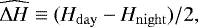 meaning that
  , and
, and  . The expansion in
 gives
gives
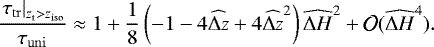 (28)
(28)
Firstly, we see that because of the symmetry of the setup, the first-order term disappears. Secondly, this readily results in a larger optical depth in the heterogeneous case than in the uniform case for all the rays with a tangent altitude that is  scale heights greater than the altitude of the isothermal region. This qualitatively explains why there is little difference in the transmittance below the altitude of the isothermal region (~ 3800 km) in Fig. 14.
Finally, when these transmittance maps are integrated vertically, we get the transmission spectra shown in Fig. 15. As expected, the effective altitude at which the atmosphere becomes opaque systematically increases when the horizontal thermal gradient is increased near the terminator.
An important point is that the spectrum for the non-uniform case – although different from the spectrum that is obtained for a uniform atmosphere with the temperature of the terminator – can be similar to the spectrum that would be obtained for a uniform but globally hotter atmosphere. It is therefore not surprising that a retrieval algorithm would be biased and would retrieve a hotter atmosphere.
 |
Fig. 14 Maps of the spectral transmittance of clear atmosphere models of HD 209458 b as a function of wavelength and altitude. The parameters are Tday = 1800 K, Tnight = 1000 K, and Piso = 10 mb, which are representative of the real planet (Parmentier et al. 2013). A low transmittance – blue shades – is representative of opaque regions deep down and a transmittance near unity – yellow – is representative of the transparent upper atmosphere. Left panel: case with a uniform upper temperature of 1400 K. Middle panel: case with a β = 15° transition region between the day and night sides. The higher opacity of the middle case is further highlighted by the right panel that shows the map of the transmittance difference between the left and the middle cases. The altitude of the top of the isothermal region is ~ 3800 km. |
 |
Fig. 15 Spatially integrated spectra of the relative transit depth (in ppm) expected for GJ 1214 b (left panel) and HD 209458 b (right panel) as a function of the day–night transition angle (β). The colour goes from red to green when β goes from 0 to 50° every 15°. The blue curve is the reference uniform case. Spectra with larger β are undistinguishable from the uniform case. The different labelled groups of curves are for our various sets of day–night temperatures. For each (Tday − Tnight) group, the temperature at the terminator of all the models – including the uniform one – is (Tday + Tnight)/2. Transit depth can be seen to increase monotonically when β decreases. |
6.3 Bias in retrieved temperatures
The last step of our analysis is to actually run a 1D retrieval procedure on the transmittance spectra obtained with our parametrized 3D atmospheric structures to assess the biases entailed by such an approach. To do so, we use the JWST simulation tool PandExo (Batalha et al. 2017) to simulate the expected uncertainties over a wavelength range of 1.0–10 μm for the duration of a single transit. For this, we combined the simulated spectra of the NIRISS/SOSS, NIRSpec/G395M, and MIRI/LRS instruments. Observed uncertainties above 10 μm were too large to have a significant impact on retrieval results and were discarded. Finally, we binned the simulated observationsto a resolution of 100 constant in wavelength. Given that we are investigating biases due to the model rather than observational noise, we here only consider the uncertainties calculated by PandExo but do not add additional noise to the mean of our simulated observations. Significant biases in the posterior distributions of retrieved parameters can occur when considering single random noise instances of the data. To correctly alleviate such noise-induced biases, one would need to combine posterior distributions of multiple noise-instance retrievals. Fortunately, Sect. 5.2 of Feng et al. (2018) shows that the combination of multiple noise-instance retrievals converges to the noise-free retrieval posterior distributions, as expected from the central limit theorem. We did not include non-Gaussian noise due to instrument or stellar systematics, as these are not currently known or are data-set dependent, or both. We therefore note that the retrieved parameter uncertainties presented here are theoretical lower limits.
For each model of our grid in temperature and day–night transition angle, we ran the spectrum through the TauREx retrieval software (Waldmann et al. 2015). Here we considered water as the only trace gas with absorption cross sections computed using the Barber et al. (2006) line list. We include Rayleigh scattering and collision-induced absorption of H2 –H2 and H2–He (Borysow et al. 2001; Borysow 2002; Rothman et al. 2013) and assumed the atmosphere to be cloud-free. The vertical temperature-pressure profile was modelled to be isothermal. A typical posterior distribution for the retrieved parameters resulting from this procedure is shown in Fig. 16, along with the simulated input spectrum and the fitted one.
The retrieved temperatures and water abundances as a function of the transition angle (β) for our GJ 1214 b case are shown in Fig. 17. Figure 18 shows the temperature result for HD 209458 b. We tested different dayside and nightside temperatures to see how planets with various irradiations would behave. To be able to compare the retrieved temperature([(]ret) in these different cases, we use the relative retrieved temperature
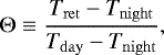 (29)
(29)
which should therefore be equal to 0.5 if we were to retrieve the terminator temperature. Although there are some quantitative differences among these cases, some robust trends emerge:
-
The retrieved temperature is systematically biased towards a higher temperature than that of the terminator (Θ ≥ 0.5).
-
There are two regimes separated by a critical day–night transition angle that depends on the characteristics of the planet and is roughly consistent with our estimate of the opening angle of the part of the planet that is probed in transit, that is, the limb (ψ, denoted by a vertical dashed line; see Fig. 2).
-
For β < ψ, the retrieved temperature decreases roughly linearly with the transition angle. As the transition angle between the dayside and nightside goes to zero (very sharp transition expected for the hottest planets), the retrieved temperature approaches the dayside temperature.
-
For β > ψ, the temperature structure within the limb, hence the retrieved temperature, does not vary significantly. Whether the actual retrieved temperature is equal to the temperature at the terminator depends on the case in question (see below).
-
Despite the uniform composition in our models, the retrieved abundance is always significantly biased – in the sense that the real abundance is outside the formal error bars of the retrieval – although the magnitude and direction depends on the specific case. It is sensible to assume that other more-complex biases will arise if chemical gradients are present as well.
If in the HD 209458 b case (see Fig. 18), the retrieved temperature converges toward the temperature at the terminator when the latter becomes more uniform (β → 180°), this is not necessarily the case for GJ 1214 b. We find that this absence of convergence at large angles always occurs when the hot, deep atmosphere below the Piso level is probed by the transit spectrum: the retrieval is biased by the vertical temperature gradient. This does not happen for our Hot Jupiter case because of the larger radius that pushes the transit photosphere at lower pressures. Although an important bias in itself, it has already been studied by Rocchetto et al. (2016), and will not be further discussed here.
 |
Fig. 16 Typical result of the retrieval procedure. This specific case is HD 209458 b with β = 15° and temperatures of 1800 and 1000 K on the dayside and nightside, respectively. Left panel: best-fit 1D spectrum (blue curve) along with the spectrum produced by our 3D tool used as input for the retrieval (black points with error bars being the 1σ uncertainty computed with PandExo). Right panel: posterior distribution for the retrieved parameters. This shows that the retrieval finds an acceptable fit, which results in relatively peaked posterior distribution and small error bars on the retrieved parameters. These values are however biased as the actual terminator temperature (1400 K) and atmospheric water abundance (log10 [H2O] = −1.3) are outside the range of values shown. |
6.4 Could we see that something is wrong?
Could an observer, having performed the retrieval, detect that the retrieved quantities are biased by the day–night temperature gradient? This is indeed a crucial point.
Unfortunately, this seems precluded, even with the exquisite precision of JWST. As can be seen in Fig. 16, the best-fit 1D, isothermal spectrum does not miss any feature of the input 3D spectrum. In fact, Fig. 19 shows that the reduced χ2 of the optimal retrieved models are always near or below unity3. Based on this metric, the 1D isothermal atmosphere model therefore provides an acceptable fit to the data, at least in the low-resolution mode that we have explored here. In fact, it even seems that the fit is better when the bias is the strongest (low day–night transition angle). This counter intuitive result comes from the fact that when the temperaturetransition is sharp, we probe almost exclusively the dayside, and the atmosphere therefore appears more homogeneous.
A procedure that would use a radiative-transfer code similar to Pythmosph3R to retrieve a 3D structure/composition (which would implyformidable computing resources) would admittedly reveal the issue as its posterior distributions would expose the full extent of the degeneracies and result in larger, more reliable error bars on the retrieved quantities. Nevertheless, such a sophisticated tool may not be able to achieve a better retrieval. Indeed, even if a better χ2 may be found with a forward model using a 3D thermal and compositional structure, the 1D model already provides an excellent match and the improvement, if any, would be achieved at the expense of adding so many parameters that parsimony criteria may favour the most simple model.
However, a much higher resolution may change this state of affairs, especially if we start to be sensitive to the line shape of individual lines. It is also possible that an east–west asymmetry of the terminator could add some signal that would be distinguishable from any 1D profile. This will have to be assessed in a future study.
7 Which atmospheres are affected?
Since the first detections of the thermal emission of a planet, the existence of a strong day–night temperature gradient on hot extrasolar planets has been well established (Cowan & Agol 2011). A clear trend has even emerged that the hotter the planet, the greater the thermal contrast (Komacek et al. 2017; Keating & Cowan 2018) – a thermal contrast that can reach more than a thousand degrees. The bias on the retrieved limb temperatures on real planets is thus potentially huge. The rather observationally unconstrained parameter, however, is the width of the day–night transition region (here β) and how it compares to the width of the limb that is effectively probed in transmission (ψ). Since phase-curve observations do not yet have the resolution necessary to precisely measure the width of the transition, we turn to published models.
For Neptune-like planets such as GJ 1214 b, our predictions based on a GCM tell us that the thermal-only effect of the day–night temperature gradient is on the order of 50–100 ppm in the water bands, and clearly detectable by JWST (see Fig. 12). It is thus sensible to assume that any hotter Neptune-like planets should be increasingly affected because of their higher H∕Rp ratio and their stronger thermal day–night contrast (see Fig. 15). On the contrary, the stratosphere of colder planets being more uniform, how cold a planet needs to be before such effects are undetectable remains to be elucidated.
However, we reiterate that only the direct thermal effect is discussed here, leaving out possible chemical heterogeneities. The strong signature of day–night gradients in the CO2 and CH4 bands of the spectrum in Fig. 12, which can reach 600–1000 ppm, are believed to be of even greater importance and could possibly strongly hamper the ability of conventional retrieval algorithms to retrieve meaningful molecular abundances in the case of heterogeneous atmospheres.
Such considerations are even more important for hot Jupiters. Despite their higher gravity, they can be much hotter, which means that the day–night contrasts are expected to be much stronger, both thermally and compositionally because chemical timescales are expected to be short compared to the advection timescales. A good example is the so-called ultra-hot Jupiters, where it is predicted that some very abundant molecules on the nightside, such as water, could be almost completely absent on the dayside due to thermal dissociation (Parmentier et al. 2018).
 |
Fig. 17 Retrieved temperature (top panel) and water abundance (bottom panel) as a function of the transition angle between the day and nightside of a planet with the radius andsurface gravity of GJ 1214 b. The colours correspond to the temperature range (blue: 300–650 K; black: 500–1000 K; red: 1000–1500 K). To put all cases on a single diagram we show the relative retrieved temperature, Θ ≡ (Tret − Tnight)/(Tday − Tnight), so that in all cases Θ = 0.5 at the terminator. The retrieved temperature is systematically biased toward the dayside temperature (Θ ≥ 0.5), especially when the transition is sharp. For comparison the estimate of the width of the limb given by Eq. (3) is shown by the vertical dotted line. |
 |
Fig. 18 Dimensionless retrieved temperature as a function of the transition angle between the dayside and nightside of a planet with the radius and surface gravity of HD 209458 b. The colours correspond to the temperature range (blue: 500–1000 K; black: 1000–1500 K; red: 1000–1800 K). See Fig. 17 for other details. |
 |
Fig. 19 Reduced χ2 for the fit of the optimal retrieved models from Figs. 17 and 18. The colour-coding is the same as for those figures. Solid curves are for GJ 1214 b and dashed are for HD 209458 b. As the reduced χ2 is always close to or smaller than 1, the fit would always be considered satisfactory. |
8 Conclusion
Overall, our most important conclusion is that the region of the atmosphere probed by transit spectroscopy, that is, the limb, is not confined to a narrow annulus around the planet as often implied, but can indeed extend relatively far throughout its two hemispheres. This is especially true for hot and/or low-gravity objects, the most significant metric being the ratio of the atmospheric scale height to the radius of the planet.
As a result, in addition to the variations of atmospheric properties of the atmosphere along the terminator, the transit spectrum is also affected by their variations across the limb, i.e. along the path of the light rays.
To investigate all these effects, we have developed Pytmosph3R, a transit spectrum generator that can work with a 3D atmospheric structure, whether it is the output of a global circulation model or a more idealised one. Using this tool along with a 3D atmospheric model of GJ 1214 b, we have recovered previous results demonstrating that the temperature and compositional variations along the terminator significantly affect the transit spectrum and will have to be accounted for in future studies. These effects can in principle be partially accounted for by using a (1+1)D, or limb-integrated, approach where one 1D spectrum is generated for each part of the limb before it is weighted and added to the others to generate the global one.
However, our fully 3D framework has shown that at the precision that will be reached by future observatories, the limb integrated approach is insufficient. Indeed, we have shown that for temperature gradients realistically expected for observable exoplanets, the transit spectrum is significantly affected by the structure of the atmosphere across the limb, that is, the thermal and compositional gradients between the dayside and nightside of the planet. We further demonstrated that this effect systematically biases 1D retrieval methods towards the temperature of the dayside. The extent of this bias, however, depends on the strengthof the temperature contrast as well as its sharpness around the terminator, the latter being the most difficult to predict.
In other words, one should be aware of the fact that the temperature (or its profile) retrieved from transmission spectra may not apply tothe terminator itself, and that temperatures at the terminator are in fact significantly smaller. This will of course be a routine problem for future high-precision observatories, but we have demonstrated that the effect on the spectrum – which canreach hundreds if not thousands of parts per million in some cases (see Fig. 15) – is well above the precision of 50–100 ppm that has been achieved with HST and Spitzer (Cowan et al. 2015). Current observations of some Hot Jupiter are therefore possibly already affected, but to what extent remains to be elucidated.
Acknowledgements
This project has received funding from the European Research Council (ERC) under the European Union’s Horizon 2020 research and innovation programme (grant agreement no. 679030/WHIPLASH, no. 758892/ ExoAI, no. 776403/ExoplANETS A and under the European Union’s Seventh Framework Programme (FP7/2007-2013)/ ERC grant agreement no. 617119/ExoLights. I.P.W. furthermore acknowledge funding by the Science and Technology Funding Council (STFC) grants: ST/K502406/1 and ST/P000282/1).
Appendix A Slant optical depth and transit radius of an isothermal, grey atmosphere with constant gravity
A.1 Homogeneous case
We first start by computing the optical depth along a ray crossing the atmosphere of a planet where temperature, gravity, and composition are constant. Here, we follow the notations of Vahidinia et al. (2014), but the reader is referred to Guillot (2010) for a more in depth discussion. Notations are summarised in Fig. 1.
The constant atmospheric scale height, H, entails that the gas number density is given by
 (A.1)
(A.1)
where n0 is the density at the reference radius (Rp). For a ray with a given tangent altitude zt, the altitude in the atmosphere at a distance x from the limb plane is given by
 (A.2)
(A.2)
to first order in zt∕Rp. The optical depth along a ray from the star to a given position x due to a given species is therefore
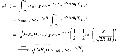 (A.3)
(A.3)
where χ is the volume mixing ration of the considered species, and σmol its cross-section at the wavelength considered. Given that the vertical optical depth is given by
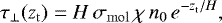 (A.4)
(A.4)
we retrieve the result from Guillot (2010) that
 (A.5)
(A.5)
Following Sect. 3.5, to first order, the transit depth is given by
 (A.6)
(A.6)
where ρ = Rp + zt. Along with Eq. (A.3), Eq. (A.6) is used to validate our model in Sect. 4.2.
A.2 Heterogeneous composition
In this section, we slightly modify the model above to answer the following question: how far from the limb plane can an increase in the abundance of a given species still affect the transit in the relevant bands? To answer this, we assume that the mixing ratio of the considered species is χday along the line ray for x < xlimb (where xlimb is negative if the transition is on the dayside) and χnight beyond that. This is supposed to mimic a situation where an absorber, such as for example TiO, becomes less abundant at the terminator and on the nightside because it condenses at cooler temperatures. Because of the symmetry of the problem, this also treats the situation where an absorber becomes more abundant on the nightside. Following Fig. 1, xlimb is also parametrized by the limb angle tan(ψ∕2) = xlimb∕(Rp + zt).
If the composition were uniform, the optical depth at a given tangent altitude would be
 (A.7)
(A.7)
Using τtr ~ 1 as a criterion for the effective altitude of absorption of the atmosphere, we get an effective altitude for the uniform case that is
 (A.8)
(A.8)
Now, in the heterogeneous case, using the penultimate line of Eq. (A.3) yields
 (A.9)
(A.9)
which is equal to the uniform case in the xlimb →−∞ limit, as expected. The effective altitude is then
 (A.10)
At what angular distance from the limb plane can we still see such an increase of a given species in the transit spectrum? To answer this question, one needs to quantify the angle ψ at which the resulting change in effective transit altitude of the atmosphere due to the heterogeneity becomes measurable. This writes
 (A.11)
where σobs is the relative precision level of the observations. Using the parameters for HD 209458 b and assuming a noise floor of 10 ppm – which is probably conservative for JWST – we see that an increase of the TiO abundance on the dayside of only a factor 100 is visible as far as 15° from the limb plane. This increase is also conservative as the abundance of TiO at temperature below 1600 K is less that 10−10 (Lodders 2002). This results in a limb width ~30° which is consistent with our other estimate (see Fig. 2).
Appendix B Finding the spherical coordinates of a cell in the cylindrical grid
To link our two coordinate systems, we use a cartesian reference frame centred around the centre of the planet and whose orthonormal reference axes are  .
.  is the unit vector along the rotation axis of the planet (pointing toward the north pole).
  points toward a reference point at the equator which will be the origin of longitudes.
  is chosen to have a direct basis. The coordinates of any point in this system are u = (X, Y, Z).
Given the position of the observer
 (B.1)
(B.1)
we need to know the physical conditions in the atmosphere at any given point u determined by its cylindrical coordinates (ρ, θ, x). For this we need to find the set of spherical coordinates (r, λ, α) corresponding to u.
This can be done by first noticing that with our definitions (see Sect. 3.1.3), u can be decomposed into a component in the plane of the sky and one along the line of sight
 (B.2)
(B.2)
where uray = (Xray, Yray, Zray) is the intersection between a (ρ, θ)-ray and the plane of the sky.
The first step is to compute Xray, Yray, and Zray. These are uniquely determined thanks to the three following definitions that can be combined into one degree-two equation:
-
since θ is the angle between the projection of the planetary rotation vector onto the plane of the sky and uray, it can be shown that Zray = ρ sinαobs cosθ;
-
uray is in the plane of the sky so that
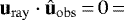 XrayXobs + YrayYobs +obs;
 -
by definition,
 .
.
Once these three components are known for each (ρ, θ), the spherical coordinates of a point are given by solving

Finally, for numerical reasons, we determine the set of indices (ir, iλ, iφ) representing this specific cell in the spherical grid.
To give a concrete example, for the simple case of a synchronous planet for which the origin of longitudes is chosen at the substellar point and observed when the star, planet, and observer are perfectly aligned, we have  Subsequently, solving the equations above yields uray (ρ, θ) = (0, ρsinθ, ρcosθ), and the corresponding relationship is

Appendix C Computing the position of the intersection of a ray with a given interface of the spherical grid
In a spherical grid, the separation between cells is done by three types of surfaces: spheres, planes of constant longitude (meridians), and cones of constant (co)latitude. Our goal is to compute the location along a ray (xint) of the intersection of this ray with any given of those surfaces. Because we know the indices of the cells before and after the intersection, we always know what type of surface we are crossing, and the value of the constant radius/longitude/colatitude identifying this surface (respectively rint, λint, and αint).
Because we also know the (ρ, θ)-ray we are dealing with, and the location of the observer, we must bear in mind that both uray = (Xray, Yray, Zray) and  are known.
The equations to be solved are the following.
-
Intersection with a sphere:
 (C.1)
(C.1)
The value is positive between the limb plane and the observer and negative otherwise.
-
Intersection with a meridian: using Eq. (B.4), we can solve for the intersection, which yields
 (C.2)
(C.2)
-
Intersection with a cone of constant colatitude: combining Eqs. (B.3) and (B.5) we get a second degree equation in xint∕ρ
 (C.3)
(C.3)
As can be seen from the equation above, the equation is the same for αint and π − αint (i.e. ± φint). This means that one cannot know a priori whether the solutions found are in the northern or southern hemisphere. In fact, when two solutions exist, the ray either intersects the cone twice in the same hemisphere (when |φobs| < |φint|), or once on each side of the equator. To remove this degeneracy, one can compute the position of the intersection of the ray with the equator xequ. Therefore, if xint > xequ the intersection is in the same hemisphere as the observer and vice versa.
Appendix D Rayleigh-scattering data
Typically, refractive indices follow the generic expression
 (D.1)
(D.1)
with terms and their values as described in Table D.1, along with the corresponding King correction factor equations. This term is taken as unity for mono-atomic gases and is calculated ab initio as described in Bates et al. (1984) for diatomic gases. The wavelength dependency of variables is also specified in Table D.1. We note that for all the formulae in this section, the wavelength is expressed in μm.
Some molecules have non-standard parametrizations. For CO2 (Sneep & Ubachs 2004)
 (D.2)
(D.2)
and
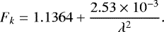 (D.3)
(D.3)
For CH4 (Sneep & Ubachs 2004)
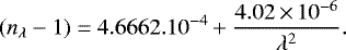 (D.4)
(D.4)
For H2O, if λ > 0.23 μm
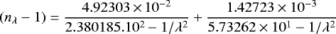 (D.5)
(D.5)
and if λ < 0.23 μm
 (D.6)
(D.6)
For molecular hydrogen we calculate the cross-section as described in Dalgarno & Williams (1962), if λ > 30 μm
 (D.7)
(D.7)
and if λ < 30 μm
 (D.8)
(D.8)
References
- Agúndez, M., Parmentier, V., Venot, O., Hersant, F., & Selsis, F. 2014, A&A, 564, A73 [NASA ADS] [CrossRef] [EDP Sciences] [Google Scholar]
- Barber, R. J., Tennyson, J., Harris, G. J., & Tolchenov, R. N. 2006, MNRAS, 368, 1087 [NASA ADS] [CrossRef] [Google Scholar]
- Batalha, N. E., Mandell, A., Pontoppidan, K., et al. 2017, PASP, 129, 064501 [NASA ADS] [CrossRef] [Google Scholar]
- Bates, R., Zarana, K. J., Tolbert, M. A., & Volkamer, R. 1984, Planet. Space Sci., 32, 785 [NASA ADS] [CrossRef] [Google Scholar]
- Beichman, C., Benneke, B., Knutson, H., et al. 2014, PASP, 126, 1134 [NASA ADS] [CrossRef] [Google Scholar]
- Blecic, J., Dobbs-Dixon, I., & Greene, T. 2017, ApJ, 848, 127 [NASA ADS] [CrossRef] [Google Scholar]
- Borysow, A. 2002, A&A, 390, 779 [NASA ADS] [CrossRef] [EDP Sciences] [Google Scholar]
- Borysow, A., Jorgensen, U. G., & Fu, Y. 2001, J. Quant. Spectr. Rad. Transf., 68, 235 [NASA ADS] [CrossRef] [Google Scholar]
- Burrows, A., Rauscher, E., Spiegel, D. S., & Menou, K. 2010, ApJ, 719, 341 [NASA ADS] [CrossRef] [Google Scholar]
- Charnay, B., Meadows, V., Misra, A., Leconte, J., & Arney, G. 2015, ApJ, 813, L1 [NASA ADS] [CrossRef] [Google Scholar]
- Chiavassa, A., Caldas, A., Selsis, F., et al. 2017, A&A, 597, A94 [NASA ADS] [CrossRef] [EDP Sciences] [Google Scholar]
- Clough, S., Kneizys, F., & Davies, R. 1989, Atm. Res., 23, 229 [NASA ADS] [CrossRef] [Google Scholar]
- Cowan, N. B.,& Agol, E. 2011, ApJ, 729, 54 [NASA ADS] [CrossRef] [Google Scholar]
- Cowan, N. B., Greene, T., Angerhausen, D., et al. 2015, PASP, 127, 311 [NASA ADS] [CrossRef] [Google Scholar]
- Dalgarno, A., & Williams, D. A. 1962, ApJ, 136, 690 [NASA ADS] [CrossRef] [Google Scholar]
- Dobbs-Dixon, I., Agol, E., & Burrows, A. 2012, ApJ, 751, 87 [NASA ADS] [CrossRef] [Google Scholar]
- Evans, T. M., Sing, D. K., Kataria, T., et al. 2017, Nature, 548, 58 [NASA ADS] [CrossRef] [Google Scholar]
- Feng, Y. K., Line, M. R., Fortney, J. J., et al. 2016, ApJ, 829, 52 [NASA ADS] [CrossRef] [Google Scholar]
- Feng, Y. K., Robinson, T. D., Fortney, J. J., et al. 2018, AJ, 155, 200 [NASA ADS] [CrossRef] [Google Scholar]
- Fortney, J. J., Shabram, M., Showman, A. P., et al. 2010, ApJ, 709, 1396 [NASA ADS] [CrossRef] [Google Scholar]
- Fu, Q., & Liou, K. N. 1992, J. Atm. Sci., 49, 2139 [NASA ADS] [CrossRef] [Google Scholar]
- Guillot, T. 2010, A&A, 520, A27 [NASA ADS] [CrossRef] [EDP Sciences] [Google Scholar]
- Hill, C., Yurchenko, S. N., & Tennyson, J. 2013, Icarus, 226, 1673 [NASA ADS] [CrossRef] [Google Scholar]
- Keating, D., & Cowan, N. B. 2018, ArXiv e-prints [arXiv:1809.00002] [Google Scholar]
- Komacek, T. D., Showman, A. P., & Tan, X. 2017, ApJ, 835, 198 [NASA ADS] [CrossRef] [Google Scholar]
- Kreidberg, L., Bean, J. L., Désert, J.-M., et al. 2014, Nature, 505, 69 [NASA ADS] [CrossRef] [Google Scholar]
- Leconte, J., Forget, F., Charnay, B., Wordsworth, R., & Pottier, A. 2013, Nature, 504, 268 [NASA ADS] [CrossRef] [Google Scholar]
- Lee, G., Dobbs-Dixon, I., Helling, C., Bognar, K., & Woitke, P. 2016, A&A, 594, A48 [NASA ADS] [CrossRef] [EDP Sciences] [Google Scholar]
- Line, M. R., & Parmentier, V. 2016, ApJ, 820, 78 [NASA ADS] [CrossRef] [Google Scholar]
- Lines, S., Manners, J., Mayne, N. J., et al. 2018, MNRAS, 481, 194 [NASA ADS] [CrossRef] [Google Scholar]
- Lodders, K. 2002, ApJ, 577, 974 [NASA ADS] [CrossRef] [Google Scholar]
- Madeleine, J.-B., Forget, F., Millour, E., Montabone, L., & Wolff, M. J. 2011, J. Geophys. Res. Planets, 116, E11010 [NASA ADS] [CrossRef] [Google Scholar]
- Madhusudhan, N. 2018, Atmospheric Retrieval of Exoplanets (Cham: Springer Publishing Company), 104 [Google Scholar]
- Miller-Ricci Kempton, E., & Rauscher, E. 2012, ApJ, 751, 117 [NASA ADS] [CrossRef] [Google Scholar]
- Parmentier, V., Showman, A. P., & Lian, Y. 2013, A&A, 558, A91 [NASA ADS] [CrossRef] [EDP Sciences] [Google Scholar]
- Parmentier, V., Line, M. R., Bean, J. L., et al. 2018, A&A, 617, A110 [NASA ADS] [CrossRef] [EDP Sciences] [Google Scholar]
- Richard, C., Gordon, I., Rothman, L., et al. 2012, J. Quant. Spectr. Rad. Transf., 113, 1276 [NASA ADS] [CrossRef] [Google Scholar]
- Rocchetto, M., Waldmann, I. P., Venot, O., Lagage, P.-O., & Tinetti, G. 2016, ApJ, 833, 120 [NASA ADS] [CrossRef] [EDP Sciences] [Google Scholar]
- Rothman, L. S., Gordon, I. E., Babikov, Y., et al. 2013, J. Quant. Spectr. Rad. Transf., 130, 4 [Google Scholar]
- Selsis, F., Wordsworth, R. D., & Forget, F. 2011, A&A, 532, A1 [NASA ADS] [CrossRef] [EDP Sciences] [Google Scholar]
- Showman, A. P., Fortney, J. J., Lewis, N. K., & Shabram, M. 2013, ApJ, 762, 24 [NASA ADS] [CrossRef] [Google Scholar]
- Sneep, M., & Ubachs, W. 2004, J. Quant. Spectr. Rad. Transf., 92, 293 [Google Scholar]
- Thalman, R., Zarzana, K. J., Tolbert, M. A., & Volkamer, R. 2014, J. Quant. Spectr. Rad. Transf., 147, 171 [NASA ADS] [CrossRef] [Google Scholar]
- Tinetti, G., Drossart, P., Eccleston, P., et al. 2017, European Planetary Science Congress, 11, EPSC2017 [Google Scholar]
- Turbet, M., Leconte, J., Selsis, F., et al. 2016, A&A, 596, A112 [NASA ADS] [CrossRef] [EDP Sciences] [Google Scholar]
- Turbet, M., Bolmont, E., Leconte, J., et al. 2018, A&A, 612, A86 [CrossRef] [EDP Sciences] [Google Scholar]
- Vahidinia, S., Cuzzi, J. N., Marley, M., & Fortney, J. 2014, ApJ, 789, L11 [NASA ADS] [CrossRef] [Google Scholar]
- Waldmann, I. P., Tinetti, G., Rocchetto, M., et al. 2015, ApJ, 802, 107 [NASA ADS] [CrossRef] [Google Scholar]
- Way, M. J., Aleinov, I., Amundsen, D. S., et al. 2017, ApJS, 231, 12 [NASA ADS] [CrossRef] [Google Scholar]
- Wordsworth, R. D., Forget, F., Selsis, F., et al. 2011, ApJ, 733, L48 [NASA ADS] [CrossRef] [Google Scholar]
The limb, as defined here, should not be confused with either (i) the limb plane, which is the plane perpendicular to the observer’s line of sight passing through the planet centre, or (ii) the terminator, which is also a plane passing through the planet centre, but which is perpendicular to the star–planet axis. The latter two are confounded only when the star, planet, and observer are aligned.
In the simple case of a planet with a null obliquity, φobs = |π∕2 − i|, where i is the orbital inclination with respect to plane of the sky. The sign depends on the convention for i. Furthermore, at conjunction, λobs = λ⋆ + π, where λ⋆ is the substellar longitude.
Finding reduced χ2 smaller than unity is allowed by the fact that, although the noise-induced uncertainty on the input spectrum is used as an input of the retrieval procedure, no noise instance has been added to the input spectrum itself (see Sect. 6.3). Contrary to the case of a comparison with real data, low χ2 here are not a sign of over-fitting.
All Tables
All Figures
|
Fig. 1 Schematic of the geometry of a light ray crossing the atmosphere. The inner circle is the arbitrary reference surface of the planet of radius Rp. The lighter-grey region is the atmosphere. The distance from the centre of the planet is r = Rp + z. A light ray is defined by its distance of closest approach to the centre of the planet, ρ, and the corresponding tangential altitude zt = ρ − Rp. The direction of the light ray defines the x direction. As we further discuss the extent of the limb along the ray, we introduce xlimb so that the absorption outside the [−xlimb, xlimb] segment is negligible in determining the transit radius, and the corresponding limb opening angle ψ. |
| In the text | |
|
Fig. 2 Simple estimate of the opening angle of the region around the terminator that affects the transmission spectrum (i.e. the limb). The contours give the opening angle in degrees as a function of the planetary radius and the atmospheric scale height of the atmosphere at 10 mb (the variation of gravity with height is accounted for). The atmosphere is assumed to become transparent above the 1 Pa pressure level. Black dots are known planets for which the radius and surface gravity are measured. Some key objects are identified. The equivalent temperature is derived from the scale height assuming an atmosphere of hydrogen and helium (solar abundances) and a surface gravity of 10 m s−2. For hot, low-gravity planets like GJ 1214 b, the limb can cover almost half the surface of the planet. |
| In the text | |
|
Fig. 3 Schematic showing the cylindrical grid (in green). Left panel: grid as seen from the observer. The pink dots are examples of (ρ, θ)-rays (to follow the Python convention used by the code, the indices given start at 0). The native GCM grid at the terminator of an example simulation is shown in black to illustrate its non-uniform vertical spacing. Right panel: the side where we can follow light rays (dashed lines) as they go horizontally from left to right. The red boxes illustrate how the x-discretisation is computedfor each ray to follow closely where it goes from one cell of the spherical grid to another. |
| In the text | |
|
Fig. 4 Absolute difference between the transit radius computed for a given number of layers and model and our reference case (integral method, isothermal, grey opacity, 50 000 layers). The dots show the results of TauREx, the dashed lines represent Pytmosph3R in its discretised version, and the solid lines are for the integral version. Results are plotted for six values of Rp ∕H that increase from top to bottom for each set of curves. The names of planets representative of these values are labelled. For Pytmosph3R, we use the results of one sector only (θ = 0°) to keep the computing time reasonable for the most resolved simulations. The axis on the right converts this radius difference into a transit depth difference in the case of GJ 1214 b (i.e. a planet of 2.6 earth radii in front of a star of 0.2 solar radii). To rescale this for any type of planet or star, we multiply by |
| In the text | |
|
Fig. 5 Decimal logarithm of the reduced chi-square for the effective radius between our 3D model and the full forward model from TauREx over a range of temperature between 200 and 2600 K and of Rp∕H between 40 and 260. As a comparison, all planets described in Fig. 4 have Rp∕H > 100. The black line shows where the reduced χ2 equals unity, i.e. where model differences become insignificant compared to the noise. We assumed an error calculated with a sun-like star at 100 lyr, 1 h of integration and JWST instruments. The same work has been done for four vertical resolutions: 50, 100, 200 and 500 layers. |
| In the text | |
|
Fig. 6 Transit spectrum generated by Pytmosph3R from the outputs of a GCM simulation of GJ 1214 b (Charnay et al. 2015). The black curve represents the effective radius obtained when accounting only for the part of the atmosphere explicitly modelled by the GCM (down to ~ 0.5 Pa). The blue curve shows the result when the model is extended by an isothermal atmosphere down to 10−4 Pa. Further lowering the pressure of the model top does not alter the spectrum. |
| In the text | |
|
Fig. 7 Colour maps showing the temperature distribution in the model atmosphere of the 100× solar metallicity simulation from Charnay et al. (2015). The inner white disc represents the inner part of the planet with a radius assumed to be equal to that of GJ 1214 b (17.600 km). Top panel: temperature at the terminator. The planet is seen from the observer during transit, the poles being at the top and bottom. Bottom panel: the star is on the left and the observer on the right on the z = 0 axis. The poles are on the x = 0 axis. From centre outward, the five solid lines are respectively the 106, 103, 1, 10−2, and 10−4 Pa pressure levels. The outer circle is there as an eye guide to highlight the non-sphericity of the planet. Temperature is well homogenised below the ~103 Pa level. Maps are to scale and show that the dayside is noticeably more vertically extended than the nightside. |
| In the text | |
|
Fig. 8 Distribution of the logarithm of the mass mixing ratio of some absorbing species at the terminator in a simulation of the atmosphere of GJ 1214 b by Charnay et al. (2015). For KCl and ZnS, only the molecules in the condensed phase are considered. The dashed (solid) black curves are the contour of unit optical depth with (without) cloud opacities at a wavelength relevant to the molecule considered (1.17 μm for CH4; 4.30 μm for CO2; 1.08 μm for KCl et ZnS). The size of the inner white disc delimiting the base of the atmosphere is reduced for clarity. The whole simulated atmosphere is shown. The two white circles delimit the region enlarged in Fig. 10. |
| In the text | |
|
Fig. 9 Decimal logarithm of the column density of some molecules in the star-observer direction for a simulation of the atmosphere of GJ 1214 b by Charnay et al. (2015). See the caption of Fig. 8 for details and notations. |
| In the text | |
|
Fig. 10 Transmittance maps obtained with the simulation of the atmosphere of GJ 1214 b depicted in Fig. 8. The region shown between the inner white disc and the outer black dotted circle is an enlargement of the region delimited bywhite circles in Fig. 8. The white dotted circle corresponds to the effective radius: the radius of the opaque disc resulting in the same overall absorption as the simulation over a homogeneous stellar disc. The maps in the upperrow are obtained with Mie scattering turned off in order to show the effect of clouds. Clouds dominate near 0.95 μm, methane is the main gaseous absorber at 1.17 μm, and carbon dioxide at 4.30 μm. |
| In the text | |
|
Fig. 11 Transit spectra computed from a 3D simulation of GJ 1214 b atmosphere by Charnay et al. (2015) with Pythmosph3R (black) and a mean profile approximation (see text). Spectra are shown with (right panels) and without (left panels) the radiative effects from the KCl and ZnS clouds. In both cases the atmosphere is extrapolated vertically beyond the top of the simulation. Cloud particle radius is fixed to 0.5 μm. The plots on the lower part show the difference between the two methods. The purple line indicates the photon noise with a JWST aperture, an exposure time of twice the transit duration and a (low) resolution of R = 100. |
| In the text | |
|
Fig. 12 As in Fig. 11 but the Pythmosph3R spectra (black) are compared here with those obtained with the limb integration approximation (red). |
| In the text | |
|
Fig. 13 Colour maps showing the temperature distribution of our model atmospheres in a plane perpendicular to the terminator for three different transition angles between a 650 K dayside and a 300 K nightside (from left to right, the day–night transition angle is β = 15, 30, and 60°). The inner white circle represents the inner part of the planet with a radius assumed to be equal to that of GJ 1214 b (17.600 km). The star is on the left and the observer on the right on the y = 0 line. From the centre outward, the five solid lines are respectively the 106, 103, 1, 10−2, and 10−4 Pa pressure levels. Below the 103 Pa level, the atmosphere is assumed to efficiently redistribute heat and is horizontally isothermal. These maps are to scale and show that the dayside is noticeably more extended than the nightside. |
| In the text | |
|
Fig. 14 Maps of the spectral transmittance of clear atmosphere models of HD 209458 b as a function of wavelength and altitude. The parameters are Tday = 1800 K, Tnight = 1000 K, and Piso = 10 mb, which are representative of the real planet (Parmentier et al. 2013). A low transmittance – blue shades – is representative of opaque regions deep down and a transmittance near unity – yellow – is representative of the transparent upper atmosphere. Left panel: case with a uniform upper temperature of 1400 K. Middle panel: case with a β = 15° transition region between the day and night sides. The higher opacity of the middle case is further highlighted by the right panel that shows the map of the transmittance difference between the left and the middle cases. The altitude of the top of the isothermal region is ~ 3800 km. |
| In the text | |
|
Fig. 15 Spatially integrated spectra of the relative transit depth (in ppm) expected for GJ 1214 b (left panel) and HD 209458 b (right panel) as a function of the day–night transition angle (β). The colour goes from red to green when β goes from 0 to 50° every 15°. The blue curve is the reference uniform case. Spectra with larger β are undistinguishable from the uniform case. The different labelled groups of curves are for our various sets of day–night temperatures. For each (Tday − Tnight) group, the temperature at the terminator of all the models – including the uniform one – is (Tday + Tnight)/2. Transit depth can be seen to increase monotonically when β decreases. |
| In the text | |
|
Fig. 16 Typical result of the retrieval procedure. This specific case is HD 209458 b with β = 15° and temperatures of 1800 and 1000 K on the dayside and nightside, respectively. Left panel: best-fit 1D spectrum (blue curve) along with the spectrum produced by our 3D tool used as input for the retrieval (black points with error bars being the 1σ uncertainty computed with PandExo). Right panel: posterior distribution for the retrieved parameters. This shows that the retrieval finds an acceptable fit, which results in relatively peaked posterior distribution and small error bars on the retrieved parameters. These values are however biased as the actual terminator temperature (1400 K) and atmospheric water abundance (log10 [H2O] = −1.3) are outside the range of values shown. |
| In the text | |
|
Fig. 17 Retrieved temperature (top panel) and water abundance (bottom panel) as a function of the transition angle between the day and nightside of a planet with the radius andsurface gravity of GJ 1214 b. The colours correspond to the temperature range (blue: 300–650 K; black: 500–1000 K; red: 1000–1500 K). To put all cases on a single diagram we show the relative retrieved temperature, Θ ≡ (Tret − Tnight)/(Tday − Tnight), so that in all cases Θ = 0.5 at the terminator. The retrieved temperature is systematically biased toward the dayside temperature (Θ ≥ 0.5), especially when the transition is sharp. For comparison the estimate of the width of the limb given by Eq. (3) is shown by the vertical dotted line. |
| In the text | |
|
Fig. 18 Dimensionless retrieved temperature as a function of the transition angle between the dayside and nightside of a planet with the radius and surface gravity of HD 209458 b. The colours correspond to the temperature range (blue: 500–1000 K; black: 1000–1500 K; red: 1000–1800 K). See Fig. 17 for other details. |
| In the text | |
|
Fig. 19 Reduced χ2 for the fit of the optimal retrieved models from Figs. 17 and 18. The colour-coding is the same as for those figures. Solid curves are for GJ 1214 b and dashed are for HD 209458 b. As the reduced χ2 is always close to or smaller than 1, the fit would always be considered satisfactory. |
| In the text | |
Current usage metrics show cumulative count of Article Views (full-text article views including HTML views, PDF and ePub downloads, according to the available data) and Abstracts Views on Vision4Press platform.
Data correspond to usage on the plateform after 2015. The current usage metrics is available 48-96 hours after online publication and is updated daily on week days.
Initial download of the metrics may take a while.