| Issue |
A&A
Volume 623, March 2019
|
|
|---|---|---|
| Article Number | A112 | |
| Number of page(s) | 25 | |
| Section | Galactic structure, stellar clusters and populations | |
| DOI | https://doi.org/10.1051/0004-6361/201833994 | |
| Published online | 13 March 2019 | |
Stellar population of Sco OB2 revealed by Gaia DR2 data⋆
INAF – Osservatorio Astronomico di Palermo G.S.Vaiana, Piazza del Parlamento 1, 90134 Palermo, Italy
e-mail: This email address is being protected from spambots. You need JavaScript enabled to view it.
Received:
31
July
2018
Accepted:
24
December
2018
Abstract
Context. The Sco OB2 association is the nearest OB association, extending over approximately 2000 square degrees on the sky. Only its brightest and most massive members are already known (from HIPPARCOS) across its entire size, while studies of its lower mass population refer only to small portions of its extent.
Aims. In this work we exploit the capabilities of Gaia DR2 measurements to search for Sco OB2 members across its entire size and down to the lowest stellar masses.
Methods. We used both Gaia astrometric (proper motions and parallaxes) and photometric measurements (integrated photometry and colors) to select association members, using minimal assumptions derived mostly from the HIPPARCOS studies. Gaia resolves small details in both the kinematics of individual Sco OB2 subgroups and their distribution with distance from the Sun. We developed methods to explore the 3D kinematics of a stellar population covering large sky areas.
Results. We find nearly 11 000 pre-main-sequence (PMS) members of Sco OB2 (with less than 3% field-star contamination), plus ∼3600 main-sequence (MS) candidate members with a larger (10–30%) field-star contamination. A higher confidence subsample of ∼9200 PMS (and ∼1340 MS) members is also selected (<1% contamination for the PMS), however this group is affected by larger (∼15%) incompleteness. We separately classify stars in compact and diffuse populations. Most members belong to one of several kinematically distinct diffuse populations, whose ensemble clearly outlines the shape of the entire association. Upper Sco is the densest region of Sco OB2. It is characterized by a complex spatial and kinematical structure and has no global pattern of motion. Other dense subclusters are found in Lower Centaurus-Crux and in Upper Centaurus-Lupus; the richest example of the latter, which has been recently identified, is coincident with the group near V1062 Sco. Most of the clustered stars appear to be younger than the diffuse PMS population, suggesting star formation in small groups that rapidly disperse and are diluted, reaching space densities lower than field stars while keeping memory of their original kinematics. We also find that the open cluster IC 2602 has a similar dynamics to Sco OB2, and its PMS members are currently evaporating and forming a diffuse (size ∼10°) halo around its double-peaked core.
Key words: open clusters and associations: individual: Sco OB2 / stars: pre-main sequence / parallaxes / proper motions
Full Tables A.1 and A.2 are only available at the CDS via anonymous ftp to cdsarc.u-strasbg.fr (130.79.128.5) or via http://cdsarc.u-strasbg.fr/viz-bin/qcat?J/A+A/623/A112
© ESO 2019
1. Introduction
Sco OB2 is the OB association nearest to the Sun. Its properties were reviewed by Preibisch & Mamajek (2008), who summarized a very large literature up to that date. Its close distance (of order of 120–160 pc), together with the low spatial density of its probable members, makes a comprehensive study of its total population very difficult. As summarized by Preibisch & Mamajek (2008), there was a decade-long debate on whether this assembly of B stars (only one O star, ζ Oph, is known to belong to the association) represents one physical entity or not. The very diluted appearance, and the similarity between the proper motion (PM) of putative members with the reflex solar motion were arguments against its real existence. The HIPPARCOS data published by de Zeeuw et al. (1999) provided however evidence in favor of a physical origin of the association, but were limited to its brightest members. As remarked by Preibisch & Mamajek (2008), most of its members are still undiscovered, if a normal initial mass function (IMF) is present. The Sco OB2 association consists of three large subassociations: Upper Sco-Cen (USC), which still has ongoing star formation in the ρ Oph dark clouds; Upper Centaurus-Lupus (UCL), which contains the Lupus dark clouds; and Lower Centaurus-Crux (LCC), which crosses the Galactic plane from N to S, which is thought to be the oldest part of Sco OB2.
The huge apparent size of Sco OB2 (approximately 80° × 30°), and its sky position toward the densest regions of the inner Galactic plane, are big obstacles for a large-scale study of its population across the entire stellar mass range. Existing large-scale surveys such as PanSTARRS (Chambers et al. 2016) or VPHAS+ (Drew et al. 2014) cover only a small fraction of the entire association. In fact, the great majority of the literature on Sco OB2 (too vast to be reviewed in this work) consists of studies of spatial regions covering only a small fraction of the association size. Even X-ray imaging surveys, such as those by Krautter et al. (1997) on Lupus or Sciortino et al. (1998) on Upper Sco yielded only 136 and 50 members, respectively, over a combined sky region of ∼10% of the total Sco OB2 extent. Studies such as Pecaut et al. (2012) or Pecaut & Mamajek (2016; PM16) on the late-type Sco OB2 population discovered less than 600 members, selected using a wide variety of methods; others like Hoogerwerf (2000) are affected by substantial field-star contamination. Instead, the Gaia observations (Gaia Collaboration 2016, 2018) are very well suited to a complete study, fulfilling the requisites of homogeneity over the entire size of the association, sufficient photometric depth to cover the entire mass range, and extremely high astrometric precision to resolve ambiguities with reflex solar motion and to avoid strong field-star contamination. Therefore, we devote this work to the study of the entire Sco OB2 association using the Gaia DR2 data. Partial studies of the region have already been presented by Wright & Mamajek (2018) using earlier Gaia DR1 data, limited to the brighter stars in the Upper-Sco region. Using Gaia DR2 data, Manara et al. (2018) have studied a small number of candidate members in the Lupus clouds, of which only five were confirmed as members; instead, Goldman et al. (2018) have reported on the discovery of more than 1800 members in the Lower Cen-Crux part of Sco OB2 down to substellar masses.
Throughout this work, we use exclusively Gaia data as much as possible, even though there are many other datasets available on this association, with a two-fold purpose: The first is maximum uniformity, since member samples assembled in previous studies do not benefit from such a uniform selection strategy as is now possible with Gaia; second, in doing this we develop and test a method for studying young clusters and associations using Gaia, which might in principle be applied to a large number of star formation regions, for which less or no auxiliary data are available to complement Gaia data.
An astrometric study of the census of a cluster or association has its roots in the kinematical coherence of their members, inherited from the bulk motion of their parent cloud. In the case of an association like Sco OB2, extended over tens of degrees in the sky, projection and depth effects become important, and have actually been exploited in the studies based on HIPPARCOS (convergent-point method), such as de Zeeuw et al. (1999) or de Bruijne (1999). We discuss in depth the reconstruction of space velocities based on the new Gaia data. Since the Gaia DR2 parallaxes (π) used in this work are much more precise than the HIPPARCOS parallaxes, some methods we discuss were not directly applicable to the HIPPARCOS data. It is also worth remarking that very young clusters are often not “kinematically simple”, but show instead evidence of multiple kinematical populations in the same sky region: some examples are found in Jeffries et al. (2014), Tobin et al. (2015), Sacco et al. (2015), or Damiani et al. (2017).
This paper is structured as follows: Sect. 2 describes the Gaia data used. Section 3 discusses analytical transformations between apparent and space velocities that are relevant in this context. Section 4 presents our criteria for member selection. Section 5 presents the selection of various Sco OB2 subpopulations based on spatial and kinematical criteria. Section 6 discusses ages of the subpopulations. Section 7 discusses the 3D structure of the association. Finally, Sect. 8 provides a concluding summary of results.
2. Gaia observations
With an estimated size of ∼2000 square degrees, and its location in the inner Galactic plane, a blind search among all Gaia DR2 sources would yield an unmanageable source list. We therefore select Gaia sources up to some maximum distance. In order to choose the distance limit, we matched the HIPPARCOS probable Sco OB2 members from de Zeeuw et al. (1999) with the Gaia DR2 catalog, keeping only Gaia sources with small relative error on parallax (i.e., π/Δπ > 10), and computed their cumulative distance distribution (Fig. 1). This shows that while ∼90% of these stars have distances d in the range 100 < d < 170 pc, a curious tail including ∼8% of stars extends as far as d ∼ 300 pc. In our search for Sco OB2 members, we decided to set an initial distance limit to 200 pc and examine later any evidence for association members between 200 and 300 pc.
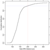 |
Fig. 1. Cumulative distribution of Gaia DR2 distances for HIPPARCOS members of Sco OB2. The vertical dotted line indicates our initial survey limit (200 pc). The horizontal dotted line indicates the percentage (92%) of HIPPARCOS members closer than this distance. |
In addition to the distance constraint, we note that the large majority (∼90%) of π measurements in Gaia DR2 are of low S/N ratio, and do not allow us to locate stars with great precision. Therefore, we also require that π/Δπ > 10 (column parallax_over_error from table gaiadr2.gaia_source), that is a relative error on π (and distance) less than 10%, for a good 3D positioning of all candidate members.
The spatial region used for selection was chosen to be slightly larger than that shown in de Zeeuw et al. (1999) and Preibisch & Mamajek (2008; their Fig. 2) to determine the boundaries of Sco OB2 in the most unbiased way. Therefore, we searched the Gaia DR2 catalog in the galactic longitude range 280 < l < 360 and galactic latitude range −10 < b < +30. This search, with the above constraints on π > 5 and π/Δπ > 10, resulted in 308 260 Gaia DR2 sources.
Besides the above filtering on parameter parallax_over_error, we experimented with the quality filters number (1) to (3) suggested by Arenou et al. (2018). Filter (1) is based on the astrometric χ2, modulated by the Gaia G magnitude of the object; filter (2) is a photometric quality filter, which is only useful if using Gaia colors; filter (3) is based on the number of Gaia observations contributing to a given measurement. It turns out however that applying filters (1) and (3) to the Gaia source list obtained above produces a rather large effect, in which only 149 141 of the sources (∼48%) pass the selection. We therefore tried to estimate whether this refinement brings a worthy improvement in our Sco OB2 Gaia source sample. Figure 2 shows the Gaia source density in the PM plane (μl, μb) in Galactic coordinates with filters (1) and (3) applied. The figure also shows the Gaia PMs of the probable Sco OB2 (HIPPARCOS) members from de Zeeuw et al. (1999), which coincide with a source density enhancement. The bulk of field sources appear rather spread across the whole PM plane and there is only a modest enhancement near (μl, μb) = (−5, 0). The red polygon encloses all HIPPARCOS members and the corresponding Gaia-source density enhancement, and therefore defines our initial member selection region.
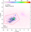 |
Fig. 2. Density plot (2D histogram) of Gaia sources in the PM plane (μl, μb) in Galactic coordinates, with parallax π > 5 and relative error on parallax π/Δπ > 10, Gaussian-smoothed, and with filters (1) and (3) applied (see Sect. 2 for details). The circle at (μl, μb) = (−40, −28) indicates the 1 − σ size of the smoothing Gaussian. The small cross at (μl, μb) = (−40, −25) represents the median PM error. Black dots indicate the HIPPARCOS Sco OB2 likely members from de Zeeuw et al. (1999). The color scale on the top axis indicates source density is in units of sources/(mas/yr)2. The red polygon enclosing all HIPPARCOS members defines the extraction region of PM-selected Gaia Sco OB2 candidate members. |
By contrast, Fig. 3 shows the Gaia source density in the same PM plane, but without filters (1) and (3) from Arenou et al. (2018). The difference is striking, especially in the bulk of field stars near (−5, 0) outside the initial selection polygon, and at the same time detailed structures inside the member-selection region are much better defined. Therefore, filtering with criteria (1) and (3) appears to be overdone especially for the field stars, and we chose not to apply these further restrictions to our initially selected Gaia sample. It is nevertheless reassuring that the fractional rejection caused by these additional filters affects likely members (inside the red polygon) much less than field stars, so that our final results are qualitatively unaffected by either choice.
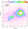 |
Fig. 3. Same as Fig. 2, but without filters (1) and (3). The same color scale is employed; densities above the range in the top-axis color bar are shown in white (e.g., the core of the field-star distribution near (−3,0)). |
Figure 2 shows also the median error on PM and the size of the smoothing Gaussian, both of which are much smaller than the distinct substructures that are evident in the density distribution of candidate members. These latter indicate therefore resolved dynamical structures of the member population, which we examine in detail in the following sections. The number of initial candidate members (inside the red polygon) is 40 512. We refer to these as PM-selected stars.
3. Space velocities
Before proceeding further, it is necessary to recall that a kinematical stellar group is defined as having a common space motion, rather than a common PM. For a compact group (less than 5–10° on the sky) there is little difference between the two representations, hence analysis in the PM plane is usually sufficient to study memberships in compact clusters. This is not true if an association of stars, such as Sco OB2 in its entirety, extends over several tens of degrees. We therefore devote this section to the development of a novel procedure (as far as we know) that is able to characterize diffuse kinematical groups in which 5D data (position, parallax, and PM) are available for each star, as in the present case.
The equations to convert sky positions (including distance R) and motion to space coordinates and velocities are
 (1)
(1)
 (2)
(2)
 (3)
(3)
then, space velocities U, V, W are
 (4)
(4)
 (5)
(5)
 (6)
(6)
These definitions of U, V, W follow the same convention adopted in many previous works (e.g., de Zeeuw et al. 1999; Dehnen & Binney 1998; Famaey et al. 2005; van Leeuwen 2009)1. Now, we have, where νR indicates radial velocity,
 (7)
(7)
 (8)
(8)
 (9)
(9)
so that the above equations transform to
 (10)
(10)
 (11)
(11)
 (12)
(12)
By simple algebraic manipulations, the latter three equations may be solved for PMs and νR, that is,
 (13)
(13)
 (14)
(14)
 (15)
(15)
The term Rμl = Vl is nothing else as the transverse velocity along l, and similarly Rμb = Vb. In Sco OB2, νR is known for only a very small percentage of members.
In the case of a spatially compact population (a few degrees on the sky), the sinl, cosl, sinb, and cosb are nearly constant, and clustering on the PM plane (and parallax) also guarantees clustering in space velocities. For diffuse populations covering many (tens of) degrees on the sky, instead, variations in the sine/cosine terms cannot be neglected. However, the specific (strong) assumption that a group of stars share the same space motion (U = U0, V = V0, W = W0) can still be tested, even if their νR values are not known. Defining ξ = tanl and ϝ = Rμl/cosl = Vl/cosl (ϝ is the greek letter “digamma”), both of which are measured for every star, we may rewrite Eq. (13) as
 (16)
(16)
which is a simple straight line in the (ξ, ϝ) plane; this is the same for all stars in a kinematical group. Conversely, a group of stars not falling along the same straight line in the (ξ, ϝ) plane cannot be a single kinematical group. The intercept and slope of the line provide space-velocity components V0 and U0, respectively. The third velocity component W0 can then be derived from Eq. (14), suitably rewritten as
 (17)
(17)
where U0 and V0 are derived from the previous step, and all other quantities on the right-hand side are measured for each star. Unlike U0 and V0, which are derived from a population best fit, W0 from Eq. (17) is computed for each star in a given group. Kinematical coherence requires that the distribution of such W0 values be sharply peaked, in order to be quantitatively consistent with the expected width of the actual W distribution (typically 1–2 km s−1) and the propagated measurement errors, which are in this case dominated by errors on parallaxes. We define this method as our method A.
We also devised an alternative method to recover (U0, V0, W0) for a diffuse kinematical population with Gaia measurements, but in the absence of measured νR. In fact, in Eqs. (10)–(12) terms l, b, R, μl, μb are all known, and those equations may be condensed as
 (18)
(18)
 (19)
(19)
 (20)
(20)
where ai and bi are constants (for each given star). These parametric equations describe a straight line in the (U, V, W) space, where νR is a parameter. For varying νR, each star corresponds to a line. For a kinematical group of stars, all the corresponding lines converge to the common point (U0, V0, W0). This method permits a simultaneous determination of all three velocity components, unlike method A above. We define this second method as method B. In its essence, it is analogous to the “spaghetti method” from Hoogerwerf & Aguilar (1999), however in a simplified form, which is justified by the much higher precision of Gaia measurements compared to HIPPARCOS.
3.1. Expansion motions
If a kinematical group expands linearly, its space velocities are
 (21)
(21)
 (22)
(22)
 (23)
(23)
where (X0, Y0, W0) is the center of expansion and k is a constant. We remark that there is circularity in this definition, since the center of expansion is defined as the (only) point in space, where (U, V, W) = (U0, V0, W0), but conversely (U0, V0, W0) is defined as the space velocity in the center of expansion. Exactly the same dynamics may be described assuming (X, Y, Z) = (0, 0, 0) as the center of expansion, and (U0 − kX0, V0 − kY0, W0 − kZ0) as its space velocity. This is a conceptual ambiguity and cannot be solved by any analysis method, as long as the velocity law is linear. By inserting the velocity laws Eqs. (21)–(23) into Eqs. (10)–(12), combined with definitions in Eqs. (1)–(3), we obtain that
 (24)
(24)
 (25)
(25)
 (26)
(26)
With the same manipulations as above, we obtain again linear relations like Eqs. (13) and (16), that is
 (27)
(27)
 (28)
(28)
which show that even in the case of linear expansion there is a linear relation between ξ and ϝ, in itself indistinguishable from that found in the absence of expansion. As Eqs. (13) and (27) show, the observed slope in the diagram (l, Vl) cannot be naively attributed to expansion or contraction, since any slope can be obtained for a suitable pair of constants (U0 − kX0, V0 − kY0) with no constraints on k. Therefore, analysis of the stellar locus in the (ξ, ϝ) plane does not by itself provide any constraint on the expansion parameter k. This is both bad news and good news. If on one hand the diagram does not permit to assess if expansion or contraction takes place (i.e., the value of k), on the other hand even a kinematical population with k ≠ 0 can be recognized as falling along a straight locus in the (ξ, ϝ) diagram. In the same way, Eq. (17) can be used to compute W0 − kZ0 once (U0 − kX0, V0 − kY0) are known, but not to derive k. More in general, careful analysis of Eqs. (24)–(26) shows that the determination of k is only possible if νR is also measured, together with the other spatial and kinematical parameters. Therefore, only a complete 6D dataset (not available for the majority of Gaia sources) can provide us with a measure of k. This coefficient is determined with the help of Eq. (15), rewritten of course as
 (29)
(29)
in whose right-hand side (V0 − kY0) and (U0 − kX0) come from the linear fit to Eq. (28), and (W0 − kZ0) from Eq. (17) rewritten as
 (30)
(30)
In this way, the quantity  can be estimated for each star, and individual measurements of νR and R (from parallax) permit us to test the existence of expansion/contraction from the correlation between
  and R and to compute the coefficient
  . A similar conclusion was reached by Blaauw (1964) and Pecaut et al. (2012).
An exception may occur if a compact cluster of stars shows a correlation between (for instance) l and Vl, suggesting expansion or contraction, and the (absolute) values of U0 or V0 implied by Eq. (27) assuming k = 0 would be unreasonably large. In this case a (rough and preliminary) estimate of k might be obtained by setting (X0, Y0) as the cluster center, and assuming U0 ∼ V0 ∼ 0, regardless of νR measurements.
4. Membership of Sco OB2
In this section, we examine the various indicators for Sco OB2 membership provided by the Gaia data, also taking advantage of the low relative error on parallaxes in the selected sample.
4.1. Color-absolute magnitude diagram
A useful diagnostic tool enabled by the accurate Gaia data is the color-absolute magnitude diagram (CAMD; shown in Fig. 4), based on Gaia BP and RP photometric measurements, and Gaia absolute G magnitude MG (see, e.g., Gaia Collaboration 2019). The error on MG introduced by parallax errors, given our selection on π/Δπ, is 0.22 mag at most and typically much less except for the faintest sources.
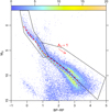 |
Fig. 4. Color-absolute magnitude diagram of all Gaia sources in our PM-selected member sample (polygon in Fig. 3). The red arrow is the reddening vector from Kounkel et al. (2018). The solid black polygon redward of BP − RP ∼ 1 defines our “PMS locus”. The solid black polygon blueward of BP − RP ∼ 1.4 defines the “Upper MS locus”. The dotted red line indicates the Pleiades sequence, while the dashed red line indicates the sequence of cluster IC 2602, both from Gaia data. |
The CAMD in Fig. 4 shows only Gaia sources in the PM-selected member sample (red polygon in Fig. 3). This diagram shows both a well-defined main sequence (MS), and a clear pre-main-sequence (PMS) band above it, separated by a gap. Also shown for reference are the empirical sequences of the Pleiades and IC 26022 clusters, which we derived using Gaia DR2 data. In the lower left part (BP − RP < 1, MG > 10) the white-dwarf sequence is also visible. The low-density, diffuse cloud of data points below the MS at colors BP − RP > 1 is due to the so-called “BP − RP excess” (e.g., Arenou et al. 2018), arising from source confusion in dense areas, for which the BP and RP colors are unreliable. In our sample this effect involves a negligible fraction of Gaia sources, even though we did not apply filter (2) from Arenou et al. (2018) that is purposely designed to remove those sources. The PMS band comprises all the low-mass members of Sco OB2, while the more massive MS members (BP − RP < 1) cannot be distinguished from the field stars from this CAMD. The red arrow represents the reddening vector, as estimated by Kounkel et al. (2018) for low extinction values; the narrow width of the MS at BP − RP < 1 (i.e., where it is not parallel to the reddening vector) shows that extinction is negligible up to the maximum sample distance of 200 pc. Exceptions to this are only likely in the immediate vicinity of dark clouds (ρ Oph, Lupus), which occupy a tiny fraction of the studied sky area. The larger solid black polygon in Fig. 4 encloses all possible PMS stars up to very young ages, and at the same time is affected by only a minimal contamination from low-mass MS field stars thanks to the MS narrow width. This polygon defines our “PMS locus” in the CAMD, and contains 10 839 sources (strongly dominated by members), reported in Table A.1, and henceforth referred to as PMS sample. The oldest ages covered by this PMS locus correspond approximately to the age of IC 2602 (∼45 Myr; e.g., Dobbie et al. 2010). The upper-MS locus of possible Sco OB2 members falls instead inside the smaller black polygon, in the upper left part of the diagram, and contains 3598 sources (both members and field stars), reported in Table A.2 and henceforth referred to as Upper-MS sample. In both Tables A.1 and A.2 we also include star identifiers from SIMBAD, when available; the match between the SIMBAD database and the Gaia DR2 catalog was made by CDS (Strasbourg) and not checked by us. Out of the 10 839 PMS members in Table A.1, only 1840 (17%) have a corresponding entry in SIMBAD; instead, a SIMBAD match is found for 2922 (81%) of the 3598 Upper-MS members in Table A.2. The PMS and Upper-MS samples are referred to collectively as the CAMD candidate member sample (14 437 stars). The CAMD of Fig. 4 also shows a modest number of red-clump giants and an even smaller number of brighter and redder giants at BP − RP > 2 and MG < 0. This type of stars cannot be a contaminant for the CAMD candidate sample.
4.2. Proper-motion diagram
The combination of photometric selection from the CAMD with astrometric selection from the PM plane provides us with a very clean sample of Sco OB2 members, especially for the (numerically dominant) low-mass PMS stars, and less cleanly for the Upper-MS stars. In fact, Fig. 5 shows the density of CAMD candidates (with no constraints on PM) in the PM plane, as in Fig. 3. The CAMD selection has the obvious effect of removing the largest majority of field stars, both near (μl, μb)∼(0, 0) and diffusely across the PM diagram (Figs. 5 and 3 have the same color scale). We estimate the residual contamination from field stars in the CAMD+PM-selected sample (i.e., the stars shown in Fig. 5 and falling inside the red box) in Sect. 4.4 below. The density distribution of CAMD candidates in the PM plane is highly structured. The comparison with median errors and width of the smoothing Gaussian kernel shows that all those structures are real, up to a level of detail even greater than that shown in Fig. 3. Fig. 5 also shows the Gaia DR2 PM data (small dots) of stars classified as Sco OB2 members by PM16 (their Table 7; henceforth “PM16 members”), matched with Gaia positions within 1 arcsec. Of the 493 PM16 members, 454 have a successful Gaia DR2 match, 451 with π > 5. Thus, only 3/454 of matched PM16 members lie farther out than 200 pc, a much smaller percentage than the de Zeeuw et al. (1999) massive candidate members (∼8%; see Sect. 2); this reinforces our arguments for a limiting distance of 200 pc in the present study. The vast majority of the PM16 members in Fig. 5 follows the same density pattern as our CAMD candidate members, as expected. However, of the 451 PM16 members with π > 5, 18 (4%) fall outside our PM-selection region (the red box in Fig. 5). There may be a variety of reasons for this, one of which may be their nature as astrometric binaries, which are not classified as such in Gaia DR2. If so, and assuming that all PM16 members are true members, we should conclude that our PM selection misses on the order of 4% of true members. However, enlarging the box further to recover them risks including too many contaminants (see below) and this option is not considered further.
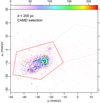 |
Fig. 5. Same as Fig. 3 (with the same color scale) for all stars in the PMS and Upper-MS loci from Fig. 4. The red polygon is the same as in Fig. 3. Dots indicate members from PM16 (their Table 7), with Gaia parallax π > 5. Outside the red polygon the density of stars is very low, but not zero. The dotted gray polygon is a reference region to estimate contamination (see Sect. 4.4). |
4.3. Transverse velocities
Some of the structures in the CAMD member distribution in Fig. 5 are in all probability related to the wide distribution of these stars in the sky, which involves non-negligible projection effects (Sect. 3). No less important than the apparent (sky-projected) space distribution is the depth distribution, suggested by a correlation (not shown for brevity) that we find between PM and parallax. In cases where the true space-velocity vector is close to normal to the line of sight, depth may become the dominant factor in the spread across the PM plane for association members. To test this, we computed transverse velocities (VT) Vl and Vb (Sect. 3), whose distribution is shown in Fig. 6 for our entire sample, and in Fig. 7 for the CAMD-selected sample. It is obvious that the candidate Sco OB2 members distribution in the latter two figures is more compact compared to that in the PM plane of Fig. 5, indicating that depth effects indeed play a major role in the apparent motion of association members. The error on Vl and Vb is often dominated by errors on π rather than on PM; we recall however that our sample was required to satisfy π/Δπ > 10, so that, on average, errors on VTs are small, as shown in the Figure, and velocity structures in the plot are real. Therefore, depth effects are not uniquely responsible for the apparent dynamical structures, and it is legitimate to investigate about other projection effects. The red polygon shown in Figs. 6 and 7 encloses the majority of Sco OB2 members and was chosen independently from that in Fig. 5. It represents a more conservative selection compared to Fig. 5. This becomes clear from a quantitative comparison between Figs. 7 and 5: in the former the red region encloses 11 058 CAMD-selected members (henceforth VT-selected members), compared to 14 437 candidate CAMD members in the latter.
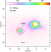 |
Fig. 6. Transverse-velocity plot (Vl, Vb) for the same sample as in Fig. 3. The median error is indicated by black segments. The solid red box encloses the majority of Sco OB2 members and was chosen independently from that in Fig. 3. The dashed red box encloses stars in IC 2602. |
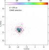 |
Fig. 7. Transverse-velocity plot (Vl, Vb), for PMS and Upper-MS stars as in Fig. 5. The red box is as in Fig. 6. Black dots represent members from PM16 as in Fig. 5. |
Figure 7 also shows the PM16 members of Sco OB2: of 451 stars with π > 5, 69 (15.3%) fall outside our selection (red polygon). We conclude that the VT-selected sample is a highly reliable, but significantly incomplete selection of association members; in the following, we consider this sample uniquely to address questions where the highest astrometric quality is involved. For general membership issues, the VT-selected sample is too much incomplete, and we prefer to consider the PM selection from Fig. 5.
Table 1 summarizes the sample statistics by subregion and adopted criteria. Numbers in column “All” are not the sum of the three preceding columns, since a (small) number of candidate members lie outside the adopted boundaries of USC, UCL, and LCC regions. From a comparison between Figs. 5 and 7 it is also clear than the VT selection leaves out IC 2602 stars, unlike PM selection. The number of IC 2602 stars from the VT diagram (and CAMD selection) is of 253 PMS and 114 Upper-MS stars, which should be added to column “LCC” of Table 1, rows 3–4, for a more accurate comparison with rows 1–2. The table shows that VT selection lowers the number of PMS candidates by 10–20%, while it operates a much more drastic reduction (>50%) on the number of Upper-MS candidates, which is again an indication of the higher nonmember contamination in the Upper-MS subsample.
Summary of candidate Sco OB2 members.
4.4. Contamination
From the previous section it is qualitatively clear that field-star contamination in the PM+CAMD sample is very small (and even less in the VT+CAMD sample). In this section, we try to quantitatively estimate this contamination. Since the spatial region we study is very large, it makes little sense to look for a comparably large sky region, where we might reasonably assume to find the same distribution of Galactic field stars but total absence of PMS stars. A reference set of measurements from which to evaluate contamination can be instead found in the PM diagram, still considering the same spatial region of our whole sample. In particular, we have shown that the largest majority of field stars across Sco OB2 (and for π > 5) are clustered around (μl, μb)∼(0, 0) in Fig. 3, and that CAMD selection rejects virtually all of these sources (Fig. 5). If we displace our selection region on the PM plane (the red polygon in Fig. 5), and recenter it to (0, 0) with a 180° rotation to avoid overlap with the current selection, we find 344 field stars inside the gray polygon in Fig. 5, also falling in the PMS region in the CAMD. This is the absolute maximum contamination that may potentially affect our PM+CAMD member sample, therefore, a maximum contamination of 3.2%. For the Upper-MS sample, the same procedure gives both a much larger number and percentage of contaminants: 1162 field stars, or 32.3%, which was qualitatively expected.
We also estimated contamination using less extreme hypotheses. For example, by rotating the red polygon in Fig. 5 by 90, 180 and 270 deg around (0, 0), we obtain, respectively, 200, 62, and 72 contaminants for the PMS sample (0.6%–1.8%), and 1068, 345, and 275 contaminants for the Upper-MS sample (7.6%–29.7%). Therefore, a rather robust conclusion is a contamination level between 1 and 3% for the PMS sample and between 10 and 30% for the Upper-MS sample.
We also considered contamination of the VT-selected samples from Fig. 7, using the same approach. By translating the red polygon to (0, 0) (absolute-maximum case) we would select 94 field stars in the PMS sample and 205 in the Upper-MS sample (1% and 15% contamination of the actual VT-selected PMS and Upper-MS samples, respectively). By rotating the selection region around (0, 0) we have 36, 4, and 16 PMS contaminants (0.04%–0.4%) and 249, 41, and 47 Upper-MS contaminants (3%–18.6%). As expected, VT selection involves a significantly lower contamination than PM selection, at the expense of a significantly lower completeness as seen above.
Therefore, the levels of contamination in these Gaia member samples are much lower than in earlier astrometric studies such as Hoogerwerf (2000), where contamination ranges from ∼30% to ∼60%, even considering our worst case of PM-selected Upper-MS members.
5. Spatial distribution of members
The sky-projected spatial density of PM-selected PMS stars is shown in Fig. 8. The total sky area of the three regions is 1974 square degrees, and the corresponding space volume up to the maximum distance surveyed here (200 pc) is 1 653 883 cubic pc. The total number of Gaia sources (after our selection on π and π/Δπ only) in the three regions is 164 042, clearly dominated by field stars; we discuss in Sect. 8 the local space density ratio of members to field stars.
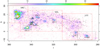 |
Fig. 8. Spatial density of PM-selected PMS stars. The top axis color bar indicates stellar density in units of stars per square degree. Pixels with densities above the color-scale maximum are shown in white. The large red dashed rectangles indicate the boundaries of the USC, UCL, and LCC regions, after de Zeeuw et al. (1999) and Preibisch & Mamajek (2008). Black dots indicate members after de Zeeuw et al. (1999). Positions of known star-forming regions from Mellinger (2008) and of the open cluster IC 2602 are indicated with labeled small circles. The dense cluster around V1062 Sco is labeled UCL-1. This and the other small clusters UCL-2, UCL-3, LCC-1, as well as IC 2602 and the Lupus III condensation are indicated by dashed rectangles. |
The highest density peaks of PMS stars in Fig. 8 (∼90 stars/square degree) are found near the ρ Oph dark cloud, and rather surprising also in correspondence to a group of stars near V1062 Sco, recently discovered by Röser et al. (2018) using Gaia DR1 data, which is labeled as UCL-1 in the figure. The global distribution of the new PMS members follows rather closely that of more massive members from de Zeeuw et al. (1999), also shown in the figure. Among the Lupus clouds, we find a noticeable density peak only in Lupus III, and a much weaker one in Lupus IV. Besides the main density peak in ρ Oph, a complex spatial structure is found all over the Upper Sco region. At the opposite extreme, we find a weaker and smoother density peak of PMS stars corresponding to the ZAMS cluster IC 2602: this is not surprising, since at the cluster age (∼45 Myr, e.g., Dobbie et al. 2010) the lowest mass stars are still found in the PMS stage and were therefore selected using our CAMD. If we had included all IC 2602 MS members, its spatial density peak would have been much higher.
Figure 8 provides many details on the lower density populations in Sco OB2. In the densest USC region, density exceeds 15 stars per square degree over a contiguous region of approximate size 15° × 15°, and exceeds 25 stars per square degree over more than one-third of the same area. There are no recognizable high-density condensations bridging the gap between this dense USC region and density peaks in UCL, such as those in the Lupus clouds and the UCL-1 cluster mentioned above. Apart from Lupus III, other subclusters in Lupus (Lupus I, II, and IV) are rather weak from the Gaia data, compared to, for example, the map in Preibisch & Mamajek (2008; their Fig. 6), and definitely weaker than other subclusters in UCL, labeled as UCL-2 and UCL-3 in Fig. 8. The mismatch between the older member map in Preibisch & Mamajek (2008) and that in Fig. 8 should not be surprising. This is because the former resulted from observations that were either spatially incomplete or with highly nonuniform depth, such as the X-ray observations in Lupus, while the Gaia data are uniform over the entire region. On the other hand, Gaia is not very sensitive to highly extincted objects, which are instead more efficiently detected using X-ray observations.
Another density peak is found in LCC, labeled as LCC-1 in the figure (containing 90 stars), together with weaker, unlabeled peaks. Besides these density peaks, the entire Sco OB2 association is permeated by a diffuse population of low-mass PMS members with densities of 5–10 stars per square degree, running without apparent discontinuity through the entire length of the association (∼70° on the sky).
The determination of kinematical groups may be severely affected by projection effects when a diffuse population spans several tens of degrees on the sky, as in this case. This does not hold for compact clusters, however. Therefore, we separate the study of compact and diffuse populations, and of their dynamics.
5.1. Compact populations
In the simplest case of a compact (on the sky) population, b ∼ const and l ∼ const., and Eqs. (13)–(16) show that Vl ∼ const and Vb ∼ const provided of course that the cluster is not elongated along the line of sight (i.e., R ∼ const., as seems reasonable). In this case projection effects are not important. Condition for the existence of a clustered and kinematically coherent population is therefore clustering both in space and on the PM or VT plane. We selected from the spatial distribution of members shown in Fig. 8 the local overdensities that most likely correspond to physical groups, well above local density fluctuations. These are indicated with dashed rectangles in the Figure. The definition of the USC compact population is discussed below (Sect. 5.1.2).
Figure 9 shows the distribution on the PM plane of compact (CAMD-selected) groups, as defined by spatial regions in Fig. 8. These distributions confirm that these spatial groups correspond to kinematically coherent populations, since most stars in each group are well localized in PM space. We consider as confirmed members in each group only stars falling inside the dashed boxes in Fig. 9. Stars from a given spatial group but falling outside of the corresponding PM box were rejected as members of the group. We find in this way 350 members (PMS+Upper-MS) in IC 2602, 593 members in UCL-1, 52 in UCL-2, 52 in UCL-3, 90 in LCC-1, and 69 in Lupus III.
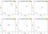 |
Fig. 9. Proper-motion diagrams of spatially compact populations (PMS and Upper-MS), as defined by dashed rectangles in Fig. 8, and no other constraints on PM. Only stars inside the dashed rectangles in the PM plane are kept as members of the respective compact populations. |
The spatial distribution of the UCL-1 population is shown in Fig. 10. As already evident from Fig. 8, this cluster is not symmetric because it is not only elongated along l, but also possessing a small “satellite” cluster (2° to the east). This small companion cluster was not detected in the discovery paper (Röser et al. 2018). A slight asymmetry was also noticeable in the PM plane (Fig. 9). UCL-1 has a likely complex internal dynamics, which deserves further studies.
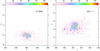 |
Fig. 10. Spatial distributions of IC 2602 (left) and UCL-1 (right) members. The spatial scale of the two panels is different. |
5.1.1. IC 2602
Figure 10 also shows the spatial distribution of PMS and Upper-MS members of IC 2602; this figure does not show the complete cluster population, which should also include lower MS members. The figure shows the presence of an extended halo (∼10−15°) around this cluster. The halo density degrades smoothly away from the cluster core, ruling out a substantial contamination by field stars. The halo has a radius much larger than the known cluster size (1.5° in radius after Kharchenko et al. 2013), and is asymmetric, being elongated along l. Although IC 2602 does not belong to Sco OB2, it is spatially and dynamically a close relative, and for this reason we include it in this work, if even marginally. The IC 2602 halo might be populated by cluster members that are gradually lost (evaporated), as is expected for all but the most tightly bound clusters (Lada & Lada 2003). While they evaporate, members keep enough memory of their original kinematics that they still contribute to the same peak in PM space as stars in the IC 2602 core. The Gaia data are therefore providing us with one rather clear detection of evaporation from a ZAMS cluster, which deserves a deeper study in a future work.
We examined if the Gaia data contain indications of a measurable expansion rate for IC 2602. We clarified in Sect. 3 that an unambiguous determination of expansion requires knowledge of radial velocities νR. We lack νR for the new Gaia members, but since IC 2602 is a well-studied cluster we know νRs for members in its core, as recently measured by Bravi et al. (2018) in the context of the Gaia-ESO Survey: from that work, the median νR is 17.63 km s−1. The Gaia data provide instead median VTs of Vl = −15.02 and Vb = 0.77 km s−1. Inserting these values into Eqs. (10)–(12) we compute median space velocities (U, V, W), which enable us to predict the locus occupied by the IC 2602 members in the (ϝ,ξ) diagram (Eq. (16)), in the absence of expansion. The resulting prediction is compared to the data in Fig. 11. If we instead use Eqs. (24)–(26) and (28), and assume an expansion rate of k = 0.05 km s−1 pc−1, we obtain a distinctly different locus on the (ϝ,ξ) plane (red line in the figure). The actual Gaia data lie somewhat in between these two cases, and deciding between them would involve a detailed membership assessment (especially) for the halo members, which requires additional data. The value k = 0.05 km s−1 pc−1 may nevertheless be considered as a robust upper limit for the IC 2602 expansion rate. This is consistent with the known age of the cluster: a star in the halo, 6° (16 pc) away from the cluster core and traveling at constant speed since 45 Myr must have a transverse speed of 0.35 km s−1, while its predicted speed with k ≤ 0.05 km s−1 pc−1 would be ≤0.8 km s−1, which is consistent with this value.
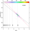 |
Fig. 11. Plot of (ϝ,ξ) for IC 2602. The dashed black and red lines are predicted loci of IC 2602 members for no expansion and expansion with k = 0.05 km s−1 pc−1, respectively. |
5.1.2. Clustered populations in Upper Sco
In the USC region the distinction between the diffuse and clustered populations is much less clear cut than elsewhere in Sco OB2. As Fig. 8 shows, the strongest density peaks in USC are surrounded by intermediate-density regions (∼30 stars per square degree) and not immediately by low-density regions (≤10 stars per square degree) as found throughout most of Sco OB2. Moreover, the high-density regions in USC do not possess regular shapes, which makes their definition even more problematic. Therefore, we devote this subsection to the definition of the clustered USC population and to the study of its peculiarities.
Figure 12 is a spatial map of all PM-selected PMS members in the USC region; we avoid Upper-MS candidates because of their larger field-star contamination. The map shows an interconnected aggregate of density peaks, of which the highest roughly corresponding to the ρ Oph dark clouds. It might be naively suspected that spatially adjacent peaks share the same dynamics (PM), but we found this not to be true. The spatial region is small enough (less than 10 × 10 square degrees as far as the high-density regions are concerned) that projection effects cannot be responsible for the difference. We therefore selected all possible high-density peaks as clustered-population candidates and then examined their dynamics. The selection was made visually and corresponds to the dashed line in Fig. 12. It defines 1045 PMS stars without constraints on PM or VT. This compact USC population is distributed on the PM plane as shown in Fig. 13: two main groups are evident, plus secondary peaks within each of them. The correspondence between position in space and in the PM plane is not trivial: for example, the three small, well-defined peaks around (l, b)∼(353, +23) do not contribute to the same group in PM space, despite their proximity on the sky. The same is found for stars near ρ Oph. The two groups in Fig. 13 are better separated along μb than along μl; therefore, we also consider their distribution on the π, μb diagram, shown in Fig. 14. This shows that, on average, the two groups have significantly different parallaxes, confirming that the two groups seen in the PM plane of Fig. 13 are real. Therefore, we conclude that there are two rather distinct compact populations in USC, which we refer to as “USC-near” (π ∼ 7) and “USC-far” (π ∼ 6−6.5). Operationally, we define their members using the two dashed regions in Fig. 14, in addition to the spatial region of Fig. 12. It should be emphasized that neither of the two subpopulations has a regular structure because there are significant substructures in both PM space and parallax. Figure 15 finally shows that substructures in USC-near and USC-far are also obviously present in their sky distribution. It is intriguing that within USC close proximity on the sky does not generally mean belonging to the same kinematical population. The number of PMS (Upper-MS) members in USC-near and -far are 501 (19) and 350 (12), respectively.
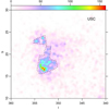 |
Fig. 12. Spatial map of PM-selected PMS stars in the USC region. The dashed line encloses the bulk of the compact component in this area. |
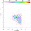 |
Fig. 14. (μb, π) diagram of the compact USC component. The dashed lines select the “USC near” and “USC far” subpopulations. |
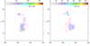 |
Fig. 15. Spatial distributions of “USC near” and “USC far” subpopulations. |
5.2. Diffuse populations
The number of Sco OB2 members found to belong to compact groups in the previous subsection is 2088 (1913 PMS and 175 Upper-MS stars). This is only 14.5% of the total number of PM+CAMD selected members: the bulk of association members are found in the diffuse population. In this section we use methods presented in Sect. 3 to study the properties of kinematical groups among this large diffuse population. We tried several methods to identify the best candidate samples for being a kinematical group. We start from the distribution on the VT plane of diffuse members, shown in Fig. 16. Still after removal of the compact populations, a complex multipeaked structure is observable in the VT plane. We might ask if projection effects can be held responsible for such a structure (as depth effects were demonstrated to be in the case of some of the structures on the PM plane), but this is unlikely the case, for at least two reasons: the association is much more elongated along l than along b, yet the two main peaks in the VT plane are no better separated along Vl than along Vb; and the spatial distribution of the (dominant) diffuse component in Sco OB2 is too smooth to produce two distinct peaks such as those in Fig. 16. Multiple peaks on the VT plane therefore correspond likely to different kinematical groups. This is further confirmed by the density plot shown in Fig. 17, showing π versus the velocity difference Vl − Vb (i.e., the projection of the velocity vector along the direction which maximizes the group differences, times  ). The richest group (labeled D2 in the figure) spans a much larger parallax range and probably consists of multiple subpopulations; the less rich group (D1) spans a smaller π range and is more likely to be a single population.
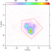 |
Fig. 16. Transverse-velocity plot (Vl, Vb), for PMS and Upper-MS stars in the diffuse component. The red box is the same as in Fig. 6. |
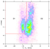 |
Fig. 17. Plot of parallax π vs. VT difference Vl − Vb. The solid red line separates diffuse components D1 and D2, as labeled. |
All diffuse populations defined in this section are required to be VT-selected members to minimize the number of possible interlopers. As a consequence, there are a number of PM-selected members falling neither in compact nor in diffuse populations, but which are still kept to avoid excessive incompleteness, as explained above. The population to which each star is assigned is also reported in Tables A.1 and A.2.
The spatial distributions of populations D1 and D2 are shown in Fig. 18. Population D1 is mostly found in UCL and nearly absent in LCC, while D2 populates all three of USC, UCL, and LCC. The density of D2 is highest in USC, and there is a hint of a density gap between USC and the rest of the D2 population. On the other hand, D2 appears to extend beyond the commonly adopted boundaries of Sco OB2, for example in the sky region 350 < l < 360 and 0 < b < 10 (hosting the cloud Barnard 59 and the Pipe Nebula).
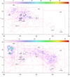 |
Fig. 18. Spatial maps of diffuse components D1 (upper panel) and D2 (lower panel). |
Adopting the formalism developed in Sect. 3, we show the (ϝ,ξ) diagram for the whole diffuse population in Fig. 19. While for l < 320 a linear dependence of ϝ on ξ (and therefore a single dynamical population) is consistent with the data, this is not the case for l > 320. This confirms that multiple dynamical populations exist, regardless of projection effects. The same diagram, for the D1 component as defined above, is shown in Fig. 20. In contrast to Fig. 19, here a linear relation between ϝ and ξ is observed, and the relative best-fit line is shown. Also shown are the positions of the compact populations, which are computed using the respective median VTs and positions. The UCL-1 and UCL-2 groups have a dynamics that is very close to the D1 diffuse component, while UCL-3 is only slightly discrepant; the dynamics of all other compact groups is much less consistent with that of population D1. As explained in Sect. 3, intercept and (negative) slope of the best-fit line to D1 provide space velocities V0 = −17.86 km s−1 and U0 = −10.11 km s−1 (Eq. (16)). Inserting these constants in Eq. (17) we obtain (star-by-star) estimates of W for population D1: this is confirmed to consist of a well-defined kinematical population if the inferred values of W fall into a narrow range. This is indeed the case, as demonstrated by the histogram of derived W values in Fig. 21, having a peak at W0 = −5.97 km s−1, and a standard deviation σW of 1.07 km s−1. The peak width is well consistent with the velocity spread commonly found in young clusters (1–2 km s−1) and we conclude that D1 is really a well-defined kinematical subpopulation according to our method A.
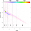 |
Fig. 19. Plot of ϝ = Vl/cosl vs. ξ = tanl for all diffuse components. Vertical dotted lines are plotted at constant l, spaced by 10°. |
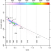 |
Fig. 20. Plot of (ϝ,ξ) for the D1 component. Vertical dotted lines as in Fig. 19. The dashed line is a linear best fit to the D1 data points. The labeled circles indicate the median (ϝ,ξ) values of the compact Sco OB2 populations. |
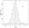 |
Fig. 21. Histogram of inferred W for the D1 population. The vertical red dashed line indicates the median W (−5.97 km s−1). |
We checked this result using our method B. To do this, we use Eqs. (18)–(20), generating for each star all possible positions (U, V, W) in velocity space for νR in the range [−25, 25] km s−1 in steps of 0.5 km s−1. Figure 22 shows the outcome of this procedure, as density of data points projected to the (V, U) and (V, W) planes in the left and right panels, respectively. In both panels, the density peak corresponds well to the values found using method A (small circles in the figure). On the (V, W) plane, method B shows some substructures in the density peak; however, they are not sufficiently separated to permit a more refined dynamical classification.
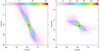 |
Fig. 22. Results of our method B, for the D1 population. Left panel: (U, V) density plot. Right panel: (W, V) density plot. In each panel, the circle indicates the result of method A. |
An analogous procedure was followed for population D2: Fig. 23 is the corresponding (ϝ,ξ) diagram. We excluded from D2 the USC region, since, as noted above, the spatial distribution of its diffuse component does not appear as a simple extension of D2 into the USC region. Even after removing the USC region, Fig. 23 shows that D2 deviates from a simple straight line at tanl ∼ −0.5. For tanl > −0.45 the diagram appearance suggests the coexistence of two populations, labeled in the figure as D2a and D2b, separated by the blue dotted line, and following distinct linear loci (dashed lines). The D2a population overlaps the tanl range of D1 (Fig. 20), but is a dynamically different population: the best-fit line for D1 is also shown in Fig. 23 (red dotted line) for comparison. D2a is instead kinematically consistent with compact groups USC-near and -far. D2b is consistent with Lupus III and slightly less with LCC-1, while it is obviously inconsistent with UCL-1 and UCL-3. For D2a we obtain best-fit values of V0 = −14.94 km s−1 and U0 = −16.2 km s−1. Again, we infer W values for its member stars, but this time we obtain a more complex W histogram, as shown in Fig. 24. The W distribution is obviously doubly-peaked and has maxima near W = −5.2 km s−1 and W = −8.75 km s−1. This is best interpreted as two populations, with nearly undistinguishable U and V components, but well-separated W components. An approximate boundary in W between the two subpopulation is adopted at W = −6.75 (dotted red line in Fig. 24). We turn to method B for a check, whose results are shown in Fig. 25, the analogous of Fig. 22. Here again, the (V, U) plane (Fig. 25, left panel) shows a single fairly well-defined peak, coincident with that found using method A; in the (V, W) plane, instead, two distinct linear streams are evident (Fig. 25, right panel), which are well consistent with the two D2a subpopulations found by method A. Again from this latter diagram, the subpopulation corresponding to peak W = −5.2 km s−1 is less rich than the other, and a complete separation between the two does not seem possible.
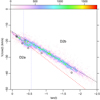 |
Fig. 23. Plot of (ϝ,ξ) for the D2 component, but excluding the USC region. Vertical dotted lines as in Fig. 19. The dotted blue line separates diffuse subpopulations D2a and D2b, whose best-fit lines are shown as dashed red and black lines, respectively. The dotted red line is the D1 best fit from Fig. 20, as a reference. The small circles are shown as in Fig. 20. |
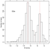 |
Fig. 24. Histogram of inferred W for the D2a population. The vertical red dashed lines are estimates of the median W for the two peaks. The boundary between the two D2a subpopulations is assumed at W = −6.75 (dotted red segment). |
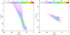 |
Fig. 25. Results of our method B, for the D2a population. Left panel: (U, V) density plot. Right panel: (W, V) density plot. In each panel, circles indicate the results of method A. |
Finally, diagrams illustrating results from methods A and B for D2b are shown in Figs. 26 and 27. In this case we obtain V0 = −14.09 km s−1 and U0 = −12.55 km s−1, and the W histogram is well behaved, with a peak (median W) at W = −7.75 and σW of 1.2 km s−1. Correspondingly, method B also indicates a single population (Fig. 27); space velocities agree with method A.
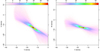 |
Fig. 27. Results of our method B, for the D2b population. Left panel: (U, V) density plot. Right panel: (W, V) density plot. In each panel, the circle indicates the result of method A. |
Total number of PMS (Upper-MS) members for D1, D2a and D2b populations are 2105 (353), 757 (145), and 3562 (640), respectively. The existence of discrete diffuse populations, each with its own well-characterized kinematical properties, as found in this work, is in contrast with the continuous dependence of (U, V, W) on l, as in Rizzuto et al. (2011). In hindsight, in Fig. 2a from Rizzuto et al., at least three layers of constant U were already noticeable. The Gaia DR2 data are much more precise than those available to those authors, so that a continuous U distribution across the entire Sco OB2 can be ruled out.
5.2.1. Diffuse population in Upper Sco
As is clear from Sect. 5.1.2, the USC region hosts populations with a complex structure, both spatially and kinematically. Once we remove the compact populations found in Sect. 5.1.2, the remaining diffuse USC population (named USC-D2, since it is a D2 subpopulation) distributes on the PM plane as shown in Fig. 28. Again, projection effects over such a limited sky region are negligible. A comparison between Figs. 28 and 13 shows that the dominant peak in this latter (USC-near, at μb < −10 mas yr−1) has no correspondence among stars in the diffuse population (Fig. 28). Conversely, only secondary peaks in Fig. 28 (at μl > −24 mas yr−1) correspond to stars in USC-far in Fig. 13. Therefore, compact and diffuse population in USC have largely nonoverlapping kinematical properties, except perhaps for the USC-far group. Nevertheless, Fig. 28 suggests the existence of kinematical substructures (or multiple subpopulations) among the diffuse USC-D2 population, analogous though not identical to compact USC populations.
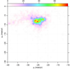 |
Fig. 28. Proper-motion diagram of the diffuse population in USC. |
Since projection effects across USC are small, our methods A and B are unlikely to provide significant indications on the space velocity vector of the USC-D2 population. We nevertheless attempted this route as above, with the results shown in Figs. 29 and 30 for method A, and Fig. 31 for method B.
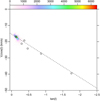 |
Fig. 29. Plot (ϝ,ξ) for the USC-D2 population. The dashed line indicates the best fit. The small circles are shown as in Fig. 20. |
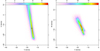 |
Fig. 31. Results of our method B, for the USC-D2 population. Left panel: (U, V) density plot. Right panel: (W, V) density plot. In each panel, the circle indicates the result of method A. |
Figure 29 show that the (ξ, ϝ) diagram for USC-D2 is somewhat wiggly, and a linear fit not very significant. The inferred W histogram of Fig. 30 is, not unexpectedly, less regular than its analogues for D1 or D2b; its σW is larger (1.54 km s−1), although still plausible. Method B confirms that results from method A are not well constrained: the locus of maximum density in the (V, U) plane (left panel in Fig. 31) is very elongated (degenerate parameters); moreover, the density distribution in the (V, W) plane possibly suggests two loci for the maxima, which are however very hard to disentangle, and only in rough agreement with results from method A. This means that the structures on the PM plane of Fig. 28 for the USC-D2 population are likely to be real, but there is no simple, nonarbitrary way to separate the subpopulations giving rise to them. Overall, USC-D2 comprises 1210 PMS and 119 Upper-MS members.
5.3. Stars beyond 200 pc
In Sect. 2 we mentioned that ∼8% of Sco OB2 members from de Zeeuw et al. (1999) have Gaia parallaxes indicating distances larger than 200 pc. However, we also found in Sect. 4.2 that only less than 1% of low-mass members from PM16 lie farther than 200 pc. In this section, we try to estimate if any significant part of Sco OB2 lies farther than this distance, which was assumed as the effective far boundary of the association in all previous sections. Therefore, we selected all Gaia sources with 3.3 < π < 5 (distance range 200–300 pc) and π/Δπ > 10 as before, together with PM-plane selection as in Sect. 2, and the requirement of falling inside the PMS locus on the CAMD3. For stars up to 200 pc, the same selection criteria resulted in the spatial map shown in Fig. 8. For the 200–300 distance range, the resulting sky distribution is instead shown in Fig. 32, shown with the same color scale as Fig. 8. The density of these (candidate PMS) stars is not uniform, with 3–4 probable concentrations (mainly near Lupus), but does not follow the spatial pattern found for Sco OB2 members. One of the most significant overdensities, as also part of the diffuse component, lie even outside the conventional association boundary. Average and peak densities are much lower than the corresponding values in Sco OB2. All these characteristics argue against these stars being association members.
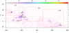 |
Fig. 32. Spatial map of PM-selected PMS candidate members having parallaxes 3.3 < π < 5 (distance between 200 and 300 pc). The color scale is the same as in Fig. 8 for an immediate comparison. |
A further indication in this sense is provided by the VT diagram for the same stars (Fig. 33). The VT diagram is preferred to the PM diagram because is compensates differences in depth, which are there by definition. The comparison between this figure and Fig. 7 shows that there is no concentration of PMS candidates between 200 and 300 pc inside the red polygon used to select Sco OB2 members; on the other hand, two distinct density peaks in the VT plane are found at larger negative Vl values, outside the red polygon. Most of the diffuse population between 200 and 300 pc is widely spread over the VT plane. If the color scale in Fig. 33 were the same as in Fig. 6, the diagram would appear as almost pure white. We conclude that there is no significant presence of Sco OB2 members beyond 200 pc. Therefore, de Zeeuw members beyond that distance are either nonmembers or perhaps runaway members. The first possibility is entirely plausible, as in Table C1 from de Zeeuw et al. (1999) 8% of the Sco OB2 members have membership probabilities P < 70%. The scarcity of PM16 members beyond 200 pc agrees well with our results.
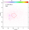 |
Fig. 33. Transverse-velocity (Vl, Vb) plot of PMS stars between 200 and 300 pc. The red box is the same as in Fig. 6. |
6. Stellar ages
An important piece of information on the star formation history in Sco OB2 is contained in the CAMD already presented in Fig. 4. In particular, the obvious gap between the MS and PMS loci shows that star formation in Sco OB2 only started less than 30–40 Myr (at most), and was essentially absent at earlier times, that is, before the birth of IC 2602, whose sequence is shown in Fig. 4. If continuous star formation were present, we would expect in the CAMD a star density inversely proportional to the speed at which a star crosses a given part of the diagram. Therefore, data points should cluster near the positions corresponding to the latest PMS stages and have the least density high up on the Hayashi track, that is the opposite of what we observe. The preselection of sources shown in our CAMD was made only from the (wide) region of the PM plane from Fig. 3. Strictly speaking, we can only rule out that the parent molecular cloud of the current Sco OB2, whose dynamical signature is seen in Fig. 3, formed stars earlier than 30 Myr ago. There might be many stars at intermediate ages (e.g., 100–300 Myr) in the same space region, but having different kinematical properties. Alternatively, the Sco OB2 parent cloud might have given birth to an earlier generation of stars, but their dynamical signatures were completely erased on timescales of less than 30–40 Myr through dynamical interactions with field stars. This latter scenario seems however less likely, if we consider the rather narrow width of the PMS locus in Fig. 4, and the well-defined spatial boundaries of the diffuse Sco OB2 population found in Fig. 8.
We examined the individual CAMDs of all kinematical populations defined in Sect. 5. Members of IC 2602 are not considered in this section. We differentiate between the spatially compact and diffuse populations. Since stellar aggregates are known to disperse with time (on average), but never condense out of a dispersed population, the diffuse Sco OB2 populations must be on average older than compact populations. This holds irrespective of our ability to trace back star positions to their birthplace, from accurate measurements of individual stellar motions.
The CAMDs of Sco OB2 stars from compact populations are shown in Fig. 34 (left panel). For each group, a nonparametric fit (lowess) was made. The same was made for the Gaia DR2 data of the Pleiades and IC 2602 (solid lines) and for the total PMS Sco OB2 population (dashed black line). The standard deviations σ(MG) (mag) around the individual best fits, and the average difference Δ(MG) (mag, positive upward) with respect to the total-population best fit were computed for each subgroup, as shown in the figure legend. The same procedure was made for the diffuse populations, and the result is shown in the right panel of the same figure. Even though we did not correct for reddening, it is clear from the figure that it cannot be responsible for the observed spread of data points.
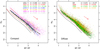 |
Fig. 34. Left panel: CAMD of stars in the compact populations; colors indicate membership. Right panel: CAMD of stars in the diffuse populations. The thin black (red) solid line indicates a best fit to the Pleiades (IC 2602) sequence, from Gaia DR2 photometry. For each population, σ (mag) is the standard deviation of datapoints around the respective best fit (colored solid lines), while Δ (mag) is the mean difference with respect to the overall best fit (thick black dashed line). The reddening vector is shown with red arrows. |
The comparison among all populations is easier if we consider the diagram in Fig. 35, which summarizes all σ and Δ values from the previous CAMDs. The youngest compact populations are (in order of increasing age) Lup-III, USC-near, and USC-far. The youngest diffuse population is USC-D2, which has both σ and Δ very close to USC-far: these two populations are closely related. The remaining diffuse populations are definitely older; the ages are not significantly different from the compact groups UCL-1, UCL-2, UCL-3, and LCC-1. The D1 and D2b populations constitute the bulk of UCL and LCC members (without one-to-one correspondence to these spatial regions, however), and their indistiguishable ages match well with results from Mamajek et al. (2002) and PM16.
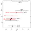 |
Fig. 35. Magnitude difference spread σ vs. average difference Δ (mags). Error bars on Δ are equal to σ. Diffuse populations are indicated in red. |
The fact that the three youngest groups are compact agrees with our above arguments that the diffuse Sco OB2 populations are on average older than the compact populations. However, it is not entirely satisfactory that a non-negligible fraction of stars in USC-near and -far are found at old apparent ages (small Δ), overlapping the bulk of stars in the D2b diffuse population. The latter is mostly located in LCC. As extensively discussed in the literature reviewed by Preibisch & Mamajek (2008), USC is thought to be the youngest part of Sco OB2; only 22 stars older than 5 Myr were found in the ρ Oph cluster by Pillitteri et al. (2016). Moreover, star formation in USC has been argued to have been triggered by events (e.g., supernova explosions) in the neighboring UCL region, itself triggered from LCC (the oldest part of Sco OB2). The presence in USC of stars as old as those in LCC does not fit in this picture. The only possibility to reconcile the commonly accepted sequence of star formation events across Sco OB2 with the incongruence described above is that individual star positions in the CAMD do not reflect (only) stellar ages. This was already proposed by Baraffe et al. (2012, 2017) and Dunham & Vorobyov (2012); see also Jeffries (2012). According to these models, the position of a star in the PMS part of the CAMD (or any equivalent of the temperature-luminosity diagram) would depend not only on its mass and age, but also on its past accretion history during the protostellar phase, which may be different from star to star. If this is true, then the large luminosity spreads we observe for USC-near and -far would have little to do with an (unlikely) spread of ages in USC, and indicate instead a wide range of past accretion histories for USC stars. It should be remarked that the individual accretion histories in a remote past are no longer traceable from (for instance) accretion or disk diagnostics currently observable, and that the star positions in the CAMD need not be altered by nonphotospheric contributions for such a scatter to take place. The large Δ(MG) for the same stars, on the other hand, would agree well with the younger ages of USC and Lupus III among all Sco OB2 populations, as reported in the literature, and suggested by their compact morphology.
The compact groups UCL-1 and UCL-3 (and UCL-2 to a lesser extent) fall in Fig. 35 close to the diffuse D1 and D2a populations, with which they are also nearly co-spatial (Fig. 18). This suggests that these clusters are nearly coeval with the diffuse population in UCL, and are what remains of the original star formation sites in that part of Sco OB2. Determining if these subclusters are bound or not would require estimates of their masses, and spatial and velocity dispersion, which were not quantitatively made.
7. Three-dimensional structure
The availability of precise parallax values (to better than 10%) for our Sco OB2 PMS members enables us to study their 3D placement in space, represented using the XYZ coordinate system. The various 2D projections of the full 3D positions are shown in Fig. 36. We show only the VT-selected members for highest reliability, from both the PMS and Upper-MS samples in panel a, and only PMS in panels b,c,d. We also include IC 2602 for comparison. Panel a is slightly smoothed to emphasize some details in the higher density regions, while the other three panels show the un-smoothed distributions to show even individual stars. Thanks to the good-quality parallaxes used, only a mild finger-of-God effect (elongated distributions toward the Sun) is noticeable. The highest density region in panel a coincides with the USC region surrounding ρ Oph, at (Y, X)∼(−15, 135), and extends almost 40 pc in depth. The second-highest concentration is found at the nearest edge of LCC, and coincides with the cluster LCC-1 at (Y, X)∼(−90, 50). This is in apparent contradiction with the density map of Fig. 8, where the second-highest density peak was at the cluster UCL-1. This is explained by observing that UCL-1 is much farther out than LCC-1, and therefore appears more compact on the sky while the latter appears “diluted”; on the contrary, shown in Fig. 36 is the true space density of stars, irrespective of projection effects. UCL-1 (at (Y, X)∼(−50, 170)) becomes thus only the third-highest density peak in real space. USC-1 and LCC-1 lie ∼125 pc apart in space, a distance which can be considered as the total length of Sco OB2. The minor peaks near (Y, X)∼(−50, 120) correspond to PMS stars in the Lupus clouds. IC 2602 is found at (Y, X)∼(−140, 50): its halo is again recognizable, and found to extend along the line of sight as it was on the sky plane (Fig. 8). A careful inspection of its spatial distribution reveals that its core is double-peaked, a fact that could only be found from Gaia precise parallaxes; the two peaks are aligned along the line of sight, and not detected in the sky projected member distribution (Fig. 8).
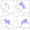 |
Fig. 36. Positions of all VT-selected PMS Sco OB2 members in Galactic XYZ coordinates. Panel a: smoothed distribution in the XY plane; unlike other panels, also Upper-MS stars are included. The Sun lies at (Y, X) = (0, 0). The directions of the Galactic center and rotation are indicated with arrows. Panels b,c,d: spatial distributions of PMS members, projected onto the YX, YZ, and XZ planes, respectively, with no smoothing applied. Density is maximum for yellow color and minimum (nonzero) for blue; white indicates zero density. |
In panels c,d of the same figure, the densest regions at Z ∼ 50 correspond to USC. The densest cluster at Z < 0 is IC 2602, while UCL-1 and LCC-1 lie at Z ∼ +15 and ∼0, respectively.
As the results from the previous section indicate, the compact and diffuse Sco OB2 populations show both similarities and differences among them, and we therefore studied their 3D distributions separately. This is done in Fig. 37, where panels in the left column show the compact groups and those on the right column the diffuse groups (VT-selected PMS only). These density plots are unsmoothed to show even individual stars. Several interesting observations may be made from these plots. The IC 2602 population was selected on the basis of (loose) spatial and PM constraints with no selection of parallax, yet Fig. 37 shows that there are at most a handful of stars in the IC 2602 group along its line of sight at random parallax values. Therefore, the number of contaminants in that sample (as far as the PMS stars are concerned) is very small. The halo around IC 2602 is therefore composed of genuine dynamical members of the cluster, and we see from the figure that it measures up to ∼40 pc in diameter. Such a large size was never suspected for that cluster in the literature, which reinforces our arguments above on cluster evaporation. Next, UCL-1 is much more distant than IC 2602, and although it appears more compact on the sky it has a comparable physical size from Fig. 37. Its small satellite lies at the same distance. Again, there are virtually no contaminant field stars all along the line of sight, even though no parallax-based selection was applied in the cluster definition. This is true of all other compact populations as well. The USC-near and -far groups were selected on the basis of their different kinematics and average parallaxes, but as noted above are not very different in terms of their spatial distribution. The two groups are largely overlapping in physical space, a puzzling result that deserves a more detailed study (possibly including spectroscopic measurements, on a larger scale than made by, e.g., Rigliaco et al. 2016).
 |
Fig. 37. Left panels: projections on the YX, YZ, and XZ planes of positions of VT-selected PMS members in compact populations. Right panels: same projections for VT-selected PMS stars in diffuse populations. |
The diffuse populations present projected spatial distributions (right column of Fig. 37) that are rather unlike those of compact groups. They are on average slightly closer to us than the compact groups (median distance for compact groups, excluding IC 2602: 155 pc; for diffuse populations: 143 pc). The diffuse populations, which were selected essentially based on their 3D kinematics, also have different distributions in space among themselves. The D1 and D2a populations lie at markedly different average distances, although there is some physical mutual overlap between them. Figure 37 shows that D1 also possesses spatial substructures, which were also suggested by our kinematical analysis using method B. The USC-D2 diffuse population in USC shows the highest degrees of spatial complexity and substructures, not an unexpected result since it bears many similarities to the compact USC populations both in kinematics (Sect. 5.2) and CAMD (Sect. 6).
We discussed in the previous section evidence that most of the diffuse populations in Sco OB2 are older than the compact ones in Lupus and USC. Therefore, Fig. 37 also suggests that star formation in Sco OB2 started in regions closer to the Sun, and then continued toward regions further away like USC, which generally agrees with literature results.
The comparison between the left and right columns of Fig. 37 shows that LCC-1 has a close connection with the D2b population, of which it might constitute a sort of remnant core. We examined the kinematical connection between Lup-III and the diffuse population in Sect. 5.2, and found that it is only compatible with D2b. This is also consistent with the respective space distributions from Fig. 37. In this case, Lup-III would nearly exactly mark the D2b boundary at large l. UCL-2 and -3 were found kinematically consistent with D1, but examining their spatial distribution this association becomes problematic for UCL-2, since D1 does not reach as far as the position of this subcluster.
8. Discussion and conclusions
We have analyzed the Gaia DR2 data on a sky region of ∼2000 square degrees containing the entire Sco OB2 association. Association members are clearly clustered on the PM and VT planes, resolving any ambiguity with the solar reflex motion that was present in earlier, lower precision astrometric data. Moreover, Gaia photometry and precise parallaxes of initial candidate members permit a clear distinction between true low-mass members, populating a clear PMS locus in the CAMD, from MS field stars; no such clear distinction is instead possible for more massive MS members of Sco OB2. The total number of PMS association members is 10 839 PMS stars, with 1–3% contamination from nonmembers, plus 3598 Upper-MS stars with a larger contamination (10–30%). A less contaminated, but less complete member sample was obtained using VTs (9221 PMS and 1337 Upper-MS stars). Of the PM-selected PMS members, 2862 fall inside the conventional boundaries of USC subassociation, 4511 in the UCL, and 2803 in LCC. This is the largest and most complete population ever found in Sco OB2, down to the bottom of the stellar mass spectrum or even below. Most of the member stars are found in a spatially diffuse component, on which local density enhancements are superimposed. The association spans a large arc, both projected on the sky and in actual space; this is in good agreement with earlier works (e.g., Sartori et al. 2003), but has much better detail. Member distances range from approximately 100 pc to almost 200 pc.
The PM and parallax distributions of members are clearly resolved thanks to the small measurement errors, and they show considerable substructures. We identified seven subclusters (plus IC 2602) that are compact both in physical and PM space. We also applied a new method to reconstruct the 3D kinematics of diffuse populations, finding four to five distinct populations with distinct spatial and kinematical properties. These do not correspond to the traditional boundaries between USC, UCL, and LCC subassociations because their spatial distributions are more complex. The most kinematically compact group is a cluster near V1062 Sco, recently discovered by Röser et al. (2018), which we named UCL-1; still, this cluster was resolved spatially (and in part, kinematically) and has a probable satellite subcluster only a few degrees away. While Röser et al. (2018) list 63 stars from Gaia DR1 data, we find a total of 593 PMS+Upper-MS members in UCL-1. The densest, but not richest part of Sco OB2 is Upper Sco, composed of an incoherent (both in PM space and in real space) assembly of local stellar groupings, lacking a well-defined global organization.
We find evidence from the CAMD that the majority (3/4) of the diffuse populations are older than compact populations in USC and Lupus. This fits with the picture of stars diffusing away rapidly from their formation sites. We find however a large spread in apparent ages from the CAMDs of the youngest groups, as if the same compact cloud had formed stars during a long period of time. This fits less well together with the age ordering based on kinematics. A possible solution that we favor is that the luminosity spread in the PMS region of the CAMD has its origin in the past accretion histories of individual stars, in agreement with recent theoretical models.
The distribution of PMS stars on the CAMD is consistent with the sequence of star formation events, from LCC and UCL to USC, reported in the literature. We find no significant age difference between the diffuse populations in LCC and UCL, in agreement with Mamajek et al. (2002) and PM16.
In our study we included, almost serendipitously, the PMS stars in the open cluster IC 2602, near the western edge of Sco OB2 and close to it on the PM plane; the parent clouds of Sco OB2 and IC 2602 might be considered as close relatives. We find that the cluster has a double core, with two distinct parallax peaks. Moreover, this cluster possesses an extended low-density halo (>10° in total size), which was never reported before to our knowledge: its detection was possible only due to the unique capabilities of Gaia.
Last, Gaia enables us to determine with accuracy the number of field stars, down to the same mass limits, which are co-spatial with Sco OB2 members, not only in sky projection but in actual 3D space. For example, we find more than 2500 MS stars in the USC region between 345 < l < 355, 12 < b < 25, and 6 < π < 8 mas, where only 1977 PMS members are found. Even worse, within the UCL sky limits and parallax limits 6.5 < π < 10 mas, more than 21000 MS field stars outnumber the 2600 PMS UCL members in the same parallax range. This means that very early during the evolution of these stars their dynamics is dominated by the general Galactic potential and not by the gravity of their coeval association members. It is interesting, however, that despite being so diffuse on the sky and spatially mixed with field stars, Sco OB2 members still keep a strong memory of their initial kinematics, which is expected to be gradually erased by dynamical friction. These data would permit an observational test of theoretical N-body models of mixing two co-spatial, but kinematically distinct star populations (e.g., Mapelli et al. 2015).
The multipeaked structure in the PM plane of stars in USC (Fig. 13), and their highly asymmetric spatial distribution (Fig. 15), suggest that turbulence and irregular geometries play a major role in determining the dynamical properties of the newly formed stars in USC, while global ordered motions are much less important. Considering an approximate USC size of 10°, and a μb dispersion ∼1.4 mas yr−1, the crossing time is tcross ∼ 25 Myr. Using the formula  (e.g., Binney & Tremaine 1987), we obtain a relaxation timescale trelax ∼ 1200 Myr, using N = 2862 from Table 1 as the number of USC members. It is likely that, before relaxation is attained, USC stars will disperse because of evaporation and the release of binding energy during gas dispersal.
There is no universal convention on the definition of U; some authors define this value as U = − dX/dt, as mentioned by Johnson & Soderblom (1987).
The IC 2602 sequence is computed from all Gaia members selected from a square sky region of 5° side centered on (RA, Dec) = (160.74167, −64.4), and with constraints π/Δπ > 10, −26 < μl < −17 mas yr−1, −2 < μb < 4 mas yr−1, and 6 < π < 7 mas (383 stars).
We checked that the larger distance of the 200–300 pc sample implies a faint limit around MG ∼ 13 on the corresponding CAMD. In Fig. 4 only 70 PMS members (∼0.6% of all PMS members) fall below that limit. Accordingly, we do not expect that the comparison between samples within and beyond 200 pc is vitiated by their different limiting MGs.
Acknowledgments
An anonymous referee made challenging yet stimulating comments which resulted in substantial improvements in the paper. This work presents results from the European Space Agency (ESA) space mission Gaia. Gaia data are being processed by the Gaia Data Processing and Analysis Consortium (DPAC). Funding for the DPAC is provided by national institutions, in particular the institutions participating in the Gaia MultiLateral Agreement (MLA). The Gaia mission website is https://www.cosmos.esa.int/gaia. The Gaia archive website is https://archives.esac.esa.int/gaia. This research makes use of the SIMBAD database and the Vizier catalog service, operated at CDS, Strasbourg, France. We also make heavy use of R: A language and environment for statistical computing. R Foundation for Statistical Computing, Vienna, Austria (http://www.R-project.org/).
References
- Arenou, F., Luri, X., Babusiaux, C., et al. 2018, A&A, 616, A17 [Google Scholar]
- Baraffe, I., Vorobyov, E., & Chabrier, G. 2012, ApJ, 756, 118 [NASA ADS] [CrossRef] [Google Scholar]
- Baraffe, I., Elbakyan, V. G., Vorobyov, E. I., & Chabrier, G. 2017, A&A, 597, A19 [NASA ADS] [CrossRef] [EDP Sciences] [Google Scholar]
- Binney, J., & Tremaine, S. 1987, Galactic Dynamics (Princeton, NJ: Princeton University Press) [Google Scholar]
- Blaauw, A. 1964, ARA&A, 2, 213 [NASA ADS] [CrossRef] [Google Scholar]
- Bravi, L., Zari, E., Sacco, G. G., et al. 2018, A&A, 615, A37 [NASA ADS] [CrossRef] [EDP Sciences] [Google Scholar]
- Chambers, K. C., Magnier, E. A., & Metcalfe, N. 2016, ArXiv e-prints [arXiv:1612.05560] [Google Scholar]
- Damiani, F., Prisinzano, L., Jeffries, R. D., et al. 2017, A&A, 602, L1 [NASA ADS] [CrossRef] [EDP Sciences] [Google Scholar]
- de Bruijne, J. H. J. 1999, MNRAS, 310, 585 [NASA ADS] [CrossRef] [Google Scholar]
- Dehnen, W., & Binney, J. J. 1998, MNRAS, 298, 387 [NASA ADS] [CrossRef] [Google Scholar]
- de Zeeuw, P. T., Hoogerwerf, R., de Bruijne, J. H. J., Brown, A. G. A., & Blaauw, A. 1999, AJ, 117, 354 [NASA ADS] [CrossRef] [Google Scholar]
- Dobbie, P. D., Lodieu, N., & Sharp, R. G. 2010, MNRAS, 409, 1002 [NASA ADS] [CrossRef] [Google Scholar]
- Drew, J. E., Gonzalez-Solares, E., Greimel, R., et al. 2014, MNRAS, 440, 2036 [NASA ADS] [CrossRef] [Google Scholar]
- Dunham, M. M., & Vorobyov, E. I. 2012, ApJ, 747, 52 [NASA ADS] [CrossRef] [Google Scholar]
- Famaey, B., Jorissen, A., Luri, X., et al. 2005, A&A, 430, 165 [NASA ADS] [CrossRef] [EDP Sciences] [Google Scholar]
- Gaia Collaboration (Prusti, T., et al.) 2016, A&A, 595, A1 [NASA ADS] [CrossRef] [EDP Sciences] [Google Scholar]
- Gaia Collaboration (Brown, A. G. A., et al.) 2018, A&A, 616, A1 [NASA ADS] [CrossRef] [EDP Sciences] [Google Scholar]
- Gaia Collaboration (Eyer, L., et al.) 2019, A&A, 623, A110 [NASA ADS] [CrossRef] [EDP Sciences] [Google Scholar]
- Goldman, B., Roeser, S., Schilbach, E., Moor, A. C., & Henning, T. 2018, ApJ, 868, 32 [NASA ADS] [CrossRef] [Google Scholar]
- Hoogerwerf, R. 2000, MNRAS, 313, 43 [NASA ADS] [CrossRef] [Google Scholar]
- Hoogerwerf, R., & Aguilar, L. A. 1999, MNRAS, 306, 394 [NASA ADS] [CrossRef] [Google Scholar]
- Jeffries, R. D. 2012, Astrophys. Space Sci. Proc., 29, 163 [NASA ADS] [CrossRef] [Google Scholar]
- Jeffries, R. D., Jackson, R. J., Cottaar, M., et al. 2014, A&A, 563, A94 [NASA ADS] [CrossRef] [EDP Sciences] [Google Scholar]
- Johnson, D. R. H., & Soderblom, D. R. 1987, AJ, 93, 864 [NASA ADS] [CrossRef] [Google Scholar]
- Kharchenko, N. V., Piskunov, A. E., Schilbach, E., Röser, S., & Scholz, R.-D. 2013, A&A, 558, A53 [NASA ADS] [CrossRef] [EDP Sciences] [Google Scholar]
- Kounkel, M., Covey, K., Suárez, G., et al. 2018, AJ, 156, 84 [NASA ADS] [CrossRef] [Google Scholar]
- Krautter, J., Wichmann, R., Schmitt, J. H. M. M., et al. 1997, A&AS, 123, 329 [NASA ADS] [CrossRef] [EDP Sciences] [Google Scholar]
- Lada, C. J., & Lada, E. A. 2003, ARA&A, 41, 57 [NASA ADS] [CrossRef] [Google Scholar]
- Mamajek, E. E., Meyer, M. R., & Liebert, J. 2002, AJ, 124, 1670 [NASA ADS] [CrossRef] [Google Scholar]
- Manara, C. F., Prusti, T., Comeron, F., et al. 2018, A&A, 615, L1 [NASA ADS] [CrossRef] [EDP Sciences] [Google Scholar]
- Mapelli, M., Vallenari, A., Jeffries, R. D., et al. 2015, A&A, 578, A35 [NASA ADS] [CrossRef] [EDP Sciences] [Google Scholar]
- Mellinger, A. 2008, Handbook of Star Forming Regions, Volume I, 4, 1 [NASA ADS] [Google Scholar]
- Pecaut, M. J., & Mamajek, E. E. 2016, MNRAS, 461, 794 [NASA ADS] [CrossRef] [Google Scholar]
- Pecaut, M. J., Mamajek, E. E., & Bubar, E. J. 2012, ApJ, 746, 154 [NASA ADS] [CrossRef] [Google Scholar]
- Pillitteri, I., Wolk, S. J., Chen, H. H., & Goodman, A. 2016, A&A, 592, A88 [NASA ADS] [CrossRef] [EDP Sciences] [Google Scholar]
- Preibisch, T., & Mamajek, E. 2008, Handbook of Star Forming Regions, 5 edn., II, 235 [NASA ADS] [Google Scholar]
- Rigliaco, E., Wilking, B., Meyer, M. R., et al. 2016, A&A, 588, A123 [NASA ADS] [CrossRef] [EDP Sciences] [Google Scholar]
- Rizzuto, A. C., Ireland, M. J., & Robertson, J. G. 2011, MNRAS, 416, 3108 [NASA ADS] [CrossRef] [Google Scholar]
- Röser, S., Schilbach, E., Goldman, B., et al. 2018, A&A, 614, A81 [NASA ADS] [CrossRef] [EDP Sciences] [Google Scholar]
- Sacco, G. G., Jeffries, R. D., Randich, S., et al. 2015, A&A, 574, L7 [NASA ADS] [CrossRef] [EDP Sciences] [Google Scholar]
- Sartori, M. J., Lépine, J. R. D., & Dias, W. S. 2003, A&A, 404, 913 [NASA ADS] [CrossRef] [EDP Sciences] [Google Scholar]
- Sciortino, S., Damiani, F., Favata, F., & Micela, G. 1998, A&A, 332, 825 [NASA ADS] [Google Scholar]
- Tobin, J. J., Hartmann, L., Fűrész, G., Hsu, W.-H., & Mateo, M. 2015, AJ, 149, 119 [NASA ADS] [CrossRef] [Google Scholar]
- van Leeuwen, F. 2009, A&A, 497, 209 [NASA ADS] [CrossRef] [EDP Sciences] [Google Scholar]
- Wright, N. J., & Mamajek, E. E. 2018, MNRAS, 476, 381 [NASA ADS] [CrossRef] [Google Scholar]
Appendix A: Additional tables
Gaia data for PMS members of Sco OB2.
Gaia data for Upper-MS members of Sco OB2.
All Tables
All Figures
|
Fig. 1. Cumulative distribution of Gaia DR2 distances for HIPPARCOS members of Sco OB2. The vertical dotted line indicates our initial survey limit (200 pc). The horizontal dotted line indicates the percentage (92%) of HIPPARCOS members closer than this distance. |
| In the text | |
|
Fig. 2. Density plot (2D histogram) of Gaia sources in the PM plane (μl, μb) in Galactic coordinates, with parallax π > 5 and relative error on parallax π/Δπ > 10, Gaussian-smoothed, and with filters (1) and (3) applied (see Sect. 2 for details). The circle at (μl, μb) = (−40, −28) indicates the 1 − σ size of the smoothing Gaussian. The small cross at (μl, μb) = (−40, −25) represents the median PM error. Black dots indicate the HIPPARCOS Sco OB2 likely members from de Zeeuw et al. (1999). The color scale on the top axis indicates source density is in units of sources/(mas/yr)2. The red polygon enclosing all HIPPARCOS members defines the extraction region of PM-selected Gaia Sco OB2 candidate members. |
| In the text | |
|
Fig. 3. Same as Fig. 2, but without filters (1) and (3). The same color scale is employed; densities above the range in the top-axis color bar are shown in white (e.g., the core of the field-star distribution near (−3,0)). |
| In the text | |
|
Fig. 4. Color-absolute magnitude diagram of all Gaia sources in our PM-selected member sample (polygon in Fig. 3). The red arrow is the reddening vector from Kounkel et al. (2018). The solid black polygon redward of BP − RP ∼ 1 defines our “PMS locus”. The solid black polygon blueward of BP − RP ∼ 1.4 defines the “Upper MS locus”. The dotted red line indicates the Pleiades sequence, while the dashed red line indicates the sequence of cluster IC 2602, both from Gaia data. |
| In the text | |
|
Fig. 5. Same as Fig. 3 (with the same color scale) for all stars in the PMS and Upper-MS loci from Fig. 4. The red polygon is the same as in Fig. 3. Dots indicate members from PM16 (their Table 7), with Gaia parallax π > 5. Outside the red polygon the density of stars is very low, but not zero. The dotted gray polygon is a reference region to estimate contamination (see Sect. 4.4). |
| In the text | |
|
Fig. 6. Transverse-velocity plot (Vl, Vb) for the same sample as in Fig. 3. The median error is indicated by black segments. The solid red box encloses the majority of Sco OB2 members and was chosen independently from that in Fig. 3. The dashed red box encloses stars in IC 2602. |
| In the text | |
|
Fig. 7. Transverse-velocity plot (Vl, Vb), for PMS and Upper-MS stars as in Fig. 5. The red box is as in Fig. 6. Black dots represent members from PM16 as in Fig. 5. |
| In the text | |
|
Fig. 8. Spatial density of PM-selected PMS stars. The top axis color bar indicates stellar density in units of stars per square degree. Pixels with densities above the color-scale maximum are shown in white. The large red dashed rectangles indicate the boundaries of the USC, UCL, and LCC regions, after de Zeeuw et al. (1999) and Preibisch & Mamajek (2008). Black dots indicate members after de Zeeuw et al. (1999). Positions of known star-forming regions from Mellinger (2008) and of the open cluster IC 2602 are indicated with labeled small circles. The dense cluster around V1062 Sco is labeled UCL-1. This and the other small clusters UCL-2, UCL-3, LCC-1, as well as IC 2602 and the Lupus III condensation are indicated by dashed rectangles. |
| In the text | |
|
Fig. 9. Proper-motion diagrams of spatially compact populations (PMS and Upper-MS), as defined by dashed rectangles in Fig. 8, and no other constraints on PM. Only stars inside the dashed rectangles in the PM plane are kept as members of the respective compact populations. |
| In the text | |
|
Fig. 10. Spatial distributions of IC 2602 (left) and UCL-1 (right) members. The spatial scale of the two panels is different. |
| In the text | |
|
Fig. 11. Plot of (ϝ,ξ) for IC 2602. The dashed black and red lines are predicted loci of IC 2602 members for no expansion and expansion with k = 0.05 km s−1 pc−1, respectively. |
| In the text | |
|
Fig. 12. Spatial map of PM-selected PMS stars in the USC region. The dashed line encloses the bulk of the compact component in this area. |
| In the text | |
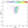 |
Fig. 13. PM diagram of the compact USC component, as defined in Fig. 12. |
| In the text | |
|
Fig. 14. (μb, π) diagram of the compact USC component. The dashed lines select the “USC near” and “USC far” subpopulations. |
| In the text | |
|
Fig. 15. Spatial distributions of “USC near” and “USC far” subpopulations. |
| In the text | |
|
Fig. 16. Transverse-velocity plot (Vl, Vb), for PMS and Upper-MS stars in the diffuse component. The red box is the same as in Fig. 6. |
| In the text | |
|
Fig. 17. Plot of parallax π vs. VT difference Vl − Vb. The solid red line separates diffuse components D1 and D2, as labeled. |
| In the text | |
|
Fig. 18. Spatial maps of diffuse components D1 (upper panel) and D2 (lower panel). |
| In the text | |
|
Fig. 19. Plot of ϝ = Vl/cosl vs. ξ = tanl for all diffuse components. Vertical dotted lines are plotted at constant l, spaced by 10°. |
| In the text | |
|
Fig. 20. Plot of (ϝ,ξ) for the D1 component. Vertical dotted lines as in Fig. 19. The dashed line is a linear best fit to the D1 data points. The labeled circles indicate the median (ϝ,ξ) values of the compact Sco OB2 populations. |
| In the text | |
|
Fig. 21. Histogram of inferred W for the D1 population. The vertical red dashed line indicates the median W (−5.97 km s−1). |
| In the text | |
|
Fig. 22. Results of our method B, for the D1 population. Left panel: (U, V) density plot. Right panel: (W, V) density plot. In each panel, the circle indicates the result of method A. |
| In the text | |
|
Fig. 23. Plot of (ϝ,ξ) for the D2 component, but excluding the USC region. Vertical dotted lines as in Fig. 19. The dotted blue line separates diffuse subpopulations D2a and D2b, whose best-fit lines are shown as dashed red and black lines, respectively. The dotted red line is the D1 best fit from Fig. 20, as a reference. The small circles are shown as in Fig. 20. |
| In the text | |
|
Fig. 24. Histogram of inferred W for the D2a population. The vertical red dashed lines are estimates of the median W for the two peaks. The boundary between the two D2a subpopulations is assumed at W = −6.75 (dotted red segment). |
| In the text | |
|
Fig. 25. Results of our method B, for the D2a population. Left panel: (U, V) density plot. Right panel: (W, V) density plot. In each panel, circles indicate the results of method A. |
| In the text | |
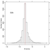 |
Fig. 26. Analogous to Fig. 21, for the D2b population. |
| In the text | |
|
Fig. 27. Results of our method B, for the D2b population. Left panel: (U, V) density plot. Right panel: (W, V) density plot. In each panel, the circle indicates the result of method A. |
| In the text | |
|
Fig. 28. Proper-motion diagram of the diffuse population in USC. |
| In the text | |
|
Fig. 29. Plot (ϝ,ξ) for the USC-D2 population. The dashed line indicates the best fit. The small circles are shown as in Fig. 20. |
| In the text | |
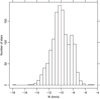 |
Fig. 30. Analogous to Fig. 21, for the USC-D2 population. |
| In the text | |
|
Fig. 31. Results of our method B, for the USC-D2 population. Left panel: (U, V) density plot. Right panel: (W, V) density plot. In each panel, the circle indicates the result of method A. |
| In the text | |
|
Fig. 32. Spatial map of PM-selected PMS candidate members having parallaxes 3.3 < π < 5 (distance between 200 and 300 pc). The color scale is the same as in Fig. 8 for an immediate comparison. |
| In the text | |
|
Fig. 33. Transverse-velocity (Vl, Vb) plot of PMS stars between 200 and 300 pc. The red box is the same as in Fig. 6. |
| In the text | |
|
Fig. 34. Left panel: CAMD of stars in the compact populations; colors indicate membership. Right panel: CAMD of stars in the diffuse populations. The thin black (red) solid line indicates a best fit to the Pleiades (IC 2602) sequence, from Gaia DR2 photometry. For each population, σ (mag) is the standard deviation of datapoints around the respective best fit (colored solid lines), while Δ (mag) is the mean difference with respect to the overall best fit (thick black dashed line). The reddening vector is shown with red arrows. |
| In the text | |
|
Fig. 35. Magnitude difference spread σ vs. average difference Δ (mags). Error bars on Δ are equal to σ. Diffuse populations are indicated in red. |
| In the text | |
|
Fig. 36. Positions of all VT-selected PMS Sco OB2 members in Galactic XYZ coordinates. Panel a: smoothed distribution in the XY plane; unlike other panels, also Upper-MS stars are included. The Sun lies at (Y, X) = (0, 0). The directions of the Galactic center and rotation are indicated with arrows. Panels b,c,d: spatial distributions of PMS members, projected onto the YX, YZ, and XZ planes, respectively, with no smoothing applied. Density is maximum for yellow color and minimum (nonzero) for blue; white indicates zero density. |
| In the text | |
|
Fig. 37. Left panels: projections on the YX, YZ, and XZ planes of positions of VT-selected PMS members in compact populations. Right panels: same projections for VT-selected PMS stars in diffuse populations. |
| In the text | |
Current usage metrics show cumulative count of Article Views (full-text article views including HTML views, PDF and ePub downloads, according to the available data) and Abstracts Views on Vision4Press platform.
Data correspond to usage on the plateform after 2015. The current usage metrics is available 48-96 hours after online publication and is updated daily on week days.
Initial download of the metrics may take a while.