| Issue |
A&A
Volume 623, March 2019
|
|
|---|---|---|
| Article Number | A70 | |
| Number of page(s) | 11 | |
| Section | Planets and planetary systems | |
| DOI | https://doi.org/10.1051/0004-6361/201833511 | |
| Published online | 07 March 2019 | |
HDO and SO2 thermal mapping on Venus
IV. Statistical analysis of the SO2 plumes
1
LESIA, Observatoire de Paris, PSL University, CNRS, Sorbonne Université, Université Sorbonne Paris Cité,
92195
Meudon,
France
e-mail: This email address is being protected from spambots. You need JavaScript enabled to view it.
2
SwRI,
Div. 15,
San Antonio,
TX
78228,
USA
3
LATMOS, IPSL,
75252
Paris, Cedex 05,
France
4
Kyoto Sangyo University,
Kyoto
603-8555,
Japan
5
LMD/IPSL, Sorbonne University, ENS, PSL University, Ecole Polytechnique, University Paris Saclay, CNRS,
75252
Paris Cedex 05,
France
6
Planetary Science Laboratory, University of Michigan,
Ann Arbor,
MI
48109-2143,
USA
7
University of Tokyo,
Kashiwa,
Chiba
277-0882,
Japan
8
Jet Propulsion Laboratory,
Pasadena,
CA
91109,
USA
9
Hokkaido Information University,
Hokkaido
069-8585,
Japan
Received:
28
May
2018
Accepted:
7
January
2019
Abstract
Since January 2012 we have been monitoring the behavior of sulfur dioxide and water on Venus, using the Texas Echelon Cross-Echelle Spectrograph (TEXES) imaging spectrometer at the NASA InfraRed Telescope Facility (IRTF, Mauna Kea Observatory). We present here the observations obtained between January 2016 and September 2018. As in the case of our previous runs, data were recorded around 1345 cm−1 (7.4 μm). The molecules SO2, CO2, and HDO (used as a proxy for H2O) were observed, and the cloudtop of Venus was probed at an altitude of about 64 km. The volume mixing ratio of SO2 was estimated using the SO2/CO2 line depth ratios of weak transitions; the H2O volume mixing ratio was derived from the HDO/CO2 line depth ratio, assuming a D/H ratio of 200 times the Vienna Standard Mean Ocean Water (VSMOW). As reported in our previous analyses, the SO2 mixing ratio shows strong variations with time and also over the disk, showing evidence of the formation of SO2 plumes with a lifetime of a few hours; in contrast, the H2O abundance is remarkably uniform over the disk and shows moderate variations as a function of time. We performed a statistical analysis of the behavior of the SO2 plumes, using all TEXES data between 2012 and 2018. They appear mostly located around the equator. Their distribution as a function of local time seems to show a depletion around noon; we do not have enough data to confirm this feature definitely. The distribution of SO2 plumes as a function of longitude shows no clear feature, apart from a possible depletion around 100E–150E and around 300E–360E. There seems to be a tendency for the H2O volume mixing ratio to decrease after 2016, and for the SO2 mixing ratio to increase after 2014. However, we see no clear anti-correlation between the SO2 and H2O abundances at the cloudtop, neither on the individual maps nor over the long term. Finally, there is a good agreement between the TEXES results and those obtained in the UV range (SPICAV/Venus Express and UVI/Akatsuki) at a slightly higher altitude. This agreement shows that SO2 observations obtained in the thermal infrared can be used to extend the local time coverage of the SO2 measurements obtained in the UV range.
Key words: planets and satellites: atmospheres / planets and satellites: terrestrial planets / infrared: planetary systems
© T. Encrenaz et al. 2019
 Open Access article, published by EDP Sciences, under the terms of the Creative Commons Attribution License (http://creativecommons.org/licenses/by/4.0), which permits unrestricted use, distribution, and reproduction in any medium, provided the original work is properly cited.
1 Introduction
Water and sulfur dioxide are known to drive the atmospheric chemistry of Venus (Krasnopolsky 1986, 2007, 2010; Mills et al. 2007; Zhang et al. 2012). Below the clouds, both species are present with volume mixing ratios of about 30 and 130 ppmv, respectively (Bézard & DeBergh 2012; Marcq et al. 2018), and at low latitudes are transported upward by Hadley convection. The SO2 molecule is photodissociated, forms SO3, and combines with water to form sulfuric acid H2SO4, which condenses to form the main component of the cloud deck. Above the cloudtop, the volume mixing ratios of H2O and SO2 drop to 1–3ppmv (Fedorova et al. 2008; Belyaev et al. 2012) and 10–1000 ppbv (Zasova et al. 1993; Marcq et al. 2013; Vandaele et al. 2017). While part of the sulfur combines with water to form H2 SO4, an extra sink is needed to explain its depletion, probably in the form of sulfur-rich aerosols within the clouds (F. Lefèvre, priv. comm.). Higher in the mesosphere, at about 90 km, another source of sulfur is needed to explain the detection of SO2 and SO in submillimeter spectra (Sandor et al. 2010, 2012).
Extended space campaigns have been performed using Pioneer Venus, the Venera spacecraft, Venus Express, and Akatsuki to better understand the sulfur and water cycles in the atmosphere of Venus, using imaging and spectroscopy in the ultraviolet and infrared ranges. As acomplement to these datasets, we have been using ground-based imaging spectroscopy in the thermal infrared since 2012 to map SO2 and H2O at the cloudtop of Venus and to monitor the behavior of these two species as a function of time, both on the short term (a few hours) and the long term (years). With respect to space data, our ground-based monitoring has the advantage of recording instantaneous images of the whole disk of Venus, allowing a simultaneous analysis of the SO2 and H2 O distributions as a function of latitude, longitude, and local hour; in addition, observations in the thermal infrared allow us to observe the night side of the planet, which is not possible in the UV range.
Results of the first runs (January 2012–January 2016) have been presented in Encrenaz et al. (2012, 2013, 2016, hereafter E12, E13, E16). Data were recorded in two spectral ranges, around 1345 cm−1 (7.4 μm) and 530 cm−1 (18.9 μm). The 7.4 μm radiation probes the cloudtop, while the 18.9 μm radiation comes from within the clouds, a few kilometers below the cloudtop. The main result of these studies is that SO2 and H2 O exhibit very different behaviors: H2O is always uniformly distributed over the disk and shows moderate variations on the long term; in contrast, the SO2 maps are most often very patchy, showing SO2 plumes which appear and disappear within a timescale of a few hours. The disk-integrated SO2 abundance shows strong variations over the long term, with a contrast factor of about 10 between the minimum value observed in February 2014 and the maximum value in January 2016 (an even higher value of the SO2 volume mixing ratio was observed in July 2018).
In this paper we first describe the observations performed between January 2016 and September 2018. In our previous analysis (E16), we presented the first part of a run performed in January 2016 (January 13–January 17, 2016). In the present paper we focus on the 7.4 μm dataset, which allows us to study the behavior of SO2 and HDO at the cloudtop. We consider the whole dataset of the January 2016 run (January 13–January 21), and the subsequent runs obtained between December 2016 and September 2018 (see Table A.1). Then we use the whole TEXES dataset (2012–2018) at 7.4 μm to perform a statistical analysis of the SO2 plumes, regarding their shape, their lifetime, and their appearance as a function of latitude, longitude, and local hour. Observations are presented and discussed in Sect. 2. In Sect. 3 we describe the statistical analysis of the SO2 plumes. In Sect. 4 we present a comparative analysis of the SO2 and H2 O volume mixing ratios. In Sect. 5 we compare our results with other measurements from Venus Express and Akatsuki. In Sect. 6 we present a summary of our conclusions. The comparative study of the SO2 maps at 7.4 and 18.9 μm, allowing a retrieval of the vertical distribution of SO2, will be performed in a subsequent paper.
2 Observations and modeling
2.1 Observations
The Texas Echelon Cross-Echelle Spectrograph (TEXES) is an imaging high-resolution infrared spectrometer in operationat the NASA InfraRed telescope Facility (Lacy et al. 2002). TEXES operates between 5 and 25 μm (400–2000 cm−1) and combines high spectral capabilities (R = 80 000 at 7 μm) and good imaging capabilities (spatial resolution around 1 arcsec). As for our previous observations, we selected the 1342–1348 cm−1 (7.4 μm) interval in order to optimize the number of weak and strong transitions of SO2, HDO, and CO2. At 1345 cm−1, the spectral resolution is 0.017 cm−1 (R = 80 000). Thelength and the width of the slit were 6.0 and 1.0 arcsec, respectively. As in the case of our previous observations, we aligned the slit along the north-south celestial axis and we shifted it from west to east with a step of half the slit width and an integration time of 2 s per position. As the diameter of Venus was always larger than the slit length, we recorded several scans successively in order to build a full map. The TEXES data cubes were calibrated using the standard radiometric method (Lacy et al. 2002, Rohlfs & Wilson 2004).
Table A.1 summarizes the TEXES observations from 2016 to 2018 obtained at 7.4 μm. The run performed in January 2016 (9 consecutive days) completes the data shown in E16.
Figure 1 shows the geometrical configurations of the disk of Venus during the six TEXES runs of 2016, 2017, and 2018. Two of the runs (January 2016 and July 2017) correspond to the morning terminator, while the others correspond to the evening terminator. As discussed in E13, these two different geometrical configurations lead to different thermal structures at high latitude.
As in our previous studies, we focus our analysis on the 1344.8–1345.4 cm−1 range, which includes several weakSO2 transitions, two weak CO2 lines, and one weak HDO line. The spectroscopic parameters of the lines used in our analysis are listed in Table 3 of E16. As discussed below (Sect. 2.2), the choice of weak transitions is mandatory for estimating the SO2 and H2 O volume mixing ratios on the basis of the SO2/CO2 and HDO/CO2 line depth ratios. Figure 2 shows examples of disk-integrated spectra recorded during each run at 7.4 μm. The SO2 and CO2 lines have the advantage of being free of telluric contamination. In contrast, it can be seen that the HDO line at 1344.899 cm−1 falls in the wing of a broad telluric absorption. As a result, the retrieval of the H2 O disk-integrated volume mixing ratio is more uncertain than the SO2 retrieval. In contrast, the quality of the H2O map should not be affected by this effect, since the telluric contamination affects all pixels of the map in the same way.
Figure 3 shows six maps of the CO2 line depth at 7.4 μm, corresponding to each of our observing runs between January 2016 and September 2018. As in the previous cases, we used the weak CO2 transition at 1345.22 cm−1. The CO2 line depth gives us information on the temperature gradient just above the level that is probed at 7.4 μm in the continuum (E13, E16). It has been noticed from previous TEXES observations that, around the polar collar, when the morning terminator is observed, the gradient becomes close to zero or even negative. In this case, the SO2 and HDO mixing ratios cannot be retrieved. It can be seen from Fig. 3 that a similar effect is also observed, although not as clearly, in our latest runs. The study of the thermal structure around the polar collar as a function of the local time will be the subject of a subsequent publication.
As in our previous 7.4 μm analyses, we obtain an estimate of the volume mixing ratios of SO2 and HDO with respect to CO2 by taking the line depth ratio of the SO2 multiplet (at 1345.3 cm−1) or the HDO transition (at 1344.9 cm−1) to the CO2 transition (at 1345.2 cm−1), as shown in Fig. 3.
Figure 4 shows the maps of the SO2 volume mixing ratio obtained from the data corresponding to Figs. 2 and 3, using the transitions mentioned above. It can be seen that a maximum of the SO2 mixing ratiois observed on July 2018.
In order to better constrain the short-term variations of the SO2 plumes, we analyzed in more detail the time sequence of nine consecutive days recorded between January 13, 2016, and January 21, 2016. The first half of this sequence was presented in E16. The entire time series of the SO2/CO2 ratio maps at 7.4 μm is shown in Fig. 5. The behavior of the SO2 plumes is analyzed below (Sect. 3.1).
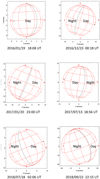 |
Fig. 1 Geometrical configurations of the disk of Venus during the six TEXES runs of 2016, 2017, and 2018. The terminator is indicated with a black line and the subsolar point with a black dot. The January 2016 and July 2017 runs correspond to the morning terminator; the four other runs correspond to the evening terminator. |
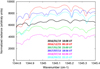 |
Fig. 2 Examples of disk-integrated spectra of Venus between 1344.8 and 1345.4 cm−1 (7.4 μm) recorded between January 2016 and September 2018. |
2.2 Atmospheric modeling
A radiative transfer model is required to convert the SO2/CO2 and HDO/CO2 line depth ratios (ldr) into SO2 and H2O volume mixing ratios (vmr). We used the same line-by-line radiative transfer code as for our previous analyses. The effect of scattering isneglected as – following the cloud model of Crisp (1986), using mode 1 and mode 2 spherical particles with a H2 SO4 concentration of 0.75 – the mean single scattering albedo is found to be 0.075 at 7.4 μm. The thermal profile in the Venus mesosphere and the spectroscopic parameters of the SO2, HDO, and CO2 transitions are described in E16. Using this model, the vmr values of SO2 and H2O at the cloudtop (in our model z = 61 km, T = 231 K, P = 100 mb) are derived from the ldr values using the following conversion factor (E16):
vmr(SO2) (ppbv) = ldr(SO2) × 600.0
vmr(H2O) (ppmv) = ldr (HDO) × 1.5
To convert the HDO vmr into the H2O vmr, we assume, following Fedorova et al. (2008), a D/H ratio of 200 times the Vienna Standard Ocean Water (VSMOW).
The validity of the conversion method is discussed in E12. Its main assumption is that, in the range of mixing ratios considered here, the line depths of the SO2, HDO, and CO2 lines used in our calculations vary linearly with the mixing ratios of these species. In the case of Mars, we show that this method is valid for line depths weaker than about ten percent (Encrenaz et al. 2008, 2015) for deriving H2 O2 and HDO vmr from the H2 O2/CO2 and HDO/CO2 ldr. In the case of Venus, we have shown that, in the 1350 cm−1 range, for SO2 and HDO lines weaker than ten percent in depth, the linearity with depth is verified with an uncertainty of about ten percent (E12).
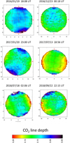 |
Fig. 3 Examples of maps of the line depth of the weak CO2 transition at 1345.22 cm−1 (7.4 μm), corresponding to the observations shown in Fig. 2. The scale is the same for the four maps. The subsolar point is shown as a white dot. |
3 Statistical study of the behavior of the SO2 plumes
Using the whole TEXES dataset between 2012 and 2018, we performed a statistical study of the SO2 plumes with respect to their lifetimes, and of their distribution as a function of latitude, longitude, and local time.
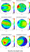 |
Fig. 4 Maps of the line depth ratio of a weak SO2 multiplet (around 1345.1 cm−1) to the CO2 transition at 1345.22 cm−1. The data are the same as in Figs. 2 and 3. The subsolar point is shown as a white dot. The scale is not the same for the six maps; the maximum SO2 abundance is observed in July 2018. |
3.1 Lifetime of the SO2 plumes
Our previous datasets (E13, E16) indicate that the typical lifetime of the SO2 plumes is about a few hours, on the basis of data recorded in July 2014, March 2015, and January 2016. Here we analyze the behavior of the SO2 plumes in more detail, on the basis of the full dataset.
We can identify two types of SO2 plumes:
-
well-localized plumes, showing an intensity as much as 4 times higher than in other areas of the disk, which appear in most of the January 2016 maps;
-
broad SO2 emissions covering a wide range of longitude; this is the case, in particular, in January 2017, July 2017, and September 2018; in July 2018, the SO2 disk-integrated intensity was at its maximum over the whole 2012–2017 dataset.
The January 2016 sequence of SO2 maps at 7.4 μm can give us some insight into the lifetime of the isolated SO2 plumes. On January 16 and 21, 2016, we see a plume appearing within a timescale of 2 h. Once a plume is formed, it tends to weaken and spread in longitude with a motion compatible with the four-day rotation of the clouds (7.5° in 2 h); this is observed on January 13, 14, 15, 17, and 19, 2016. In other cases, the SO2 plume disappears or weakens within two hours (January 20, 2016). Using the January 2016 dataset, we can observe that the lifetime of the SO2 is definitely shorter than 24 h; there is no example of a SO2 observed on a given day and still present at a longitude shifted by 90W the next day. In other words, the SO2 maps show no memory of the SO2 distribution found the previous day. It should be noted that this result is consistent with the timescale of 5 × 10⁴ s derived by Marcq et al. (2013) near the equator.
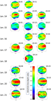 |
Fig. 5 Maps of the SO2/CO2 line depth ratio, using SO2 multiplets (around 1345.1 and 1345.3 cm−1) divided by the CO2 transition at 1345.22 cm−1, between January 13, 2016, and January 21, 2016. The subsolar point is shown as a white dot. |
3.2 Distribution of the SO2 plumes as a function of latitude
We selected a list of 34 SO2 maps at 7.4 μm, one per day. For each day, we selected the map corresponding to the maximum intensity of the SO2 plume and noted the location of the SO2 maximum versus latitude, longitude, and local time. Table 1 lists the observations used for the present study. The SO2 volume mixing indicated for each map refers to the maximum value at the center of the plume. We considered a single map per day in order to avoid the duplication of a given SO2 plume over several hours. Since the SO2 lifetime is significantly shorter than a day, we can consider all 34 maps as independent measurements.
We wondered whether our analysis might be affected by an airmass effect, as the altitude probed by the observations depends upon the emission angle. Our previous analysis (E13) showed that the SO2 vertical distribution decreases above the cloudtop as the altitude increases, so this effect would tend to enhance the measured SO2 mixing ratio at the disk center where the deepest levels are probed. However, the SO2 maps retrieved from our observations do not show this effect: there is no evidence for a SO2 enhancement at the disk center. The reason is probably that the SO2 horizontal variations over the disk are usually much larger than the vertical SO2 variations induced by the emission angle variations.
Figure 6 shows the distribution of the SO2 plumes as a function of latitude. It can be seen that the distribution strongly peaks toward the equator, with most of the features appearing within the 30N–30S latitude range. We must remember that the identification of plumes at high latitude, outside the (60N,60S) range, may be uncertain due to the peculiar shape of the thermal profile around the polar collar when the morning terminator is observed. In this case, when the thermal profile becomes close to isothermal, the retrieval of SO2 and HDO is no longer possible because the SO2 and CO2 line depths become very small. For this reason, in the following analysis, we limit our study to the SO2 plumes located within 30° of the equator.
An interesting feature was observed during our run of July 2017. Figure 7 shows four SO2 maps, two for July 12 and two for July 13, each subset separated in time by 3 h. The maps of July 12 exhibit a double structure, symmetrical with respect to the equator, extending at high northern and southern latitudes. A few other maps (January 16 and 19, 2016, Fig. 5; September 24, 2018) seem to show a similar trend.
Summary of TEXES observations used for the analysis of the SO2 plumes (2012–2018).
3.3 Distribution of the SO2 plumes as a function of longitude
For each observation listed in Table 1, we calculated the longitude range available in the field of view, and measured the longitude range covered by the SO2 plume listed in Table 1. It should be noted that the peak longitude of the SO2 plume is easy to define, whereas its width may be more difficult to determine. In the case of a patchy, highly contrasted SO2 distribution over the disk (as shown in Fig. 4 on December 23, 2016, for instance), we used the FWHM of the SO2 plume. In cases where the SO2 distribution was more extended (as in Fig. 4 for January 30 and July 13, 2017) we used a longitude range narrower than the FWHM to better isolate the maximum longitude. For each day, we selected the map showing the strongest SO2 plume and, within the disk, in case of multiple features, we chose the position of the strongest plume.
We then added all observable longitude ranges to obtain the longitude visibility curve corresponding to our dataset. We added in the same way all longitude ranges where a SO2 plume was present. Dividing this curve by the longitude visibility curve gives us the probability of SO2 appearance as a function of the longitude. Results are shown in Figs. 8 and 9. It can be seen (Fig. 8) that the longitude 100E–200E range is less observed than the 300E–50E range in theopposite hemisphere by a factor of about 2. Figure 9 shows the probability of SO2 plume appearance as a function of longitude. Two regions, one located at 100E–150E and the other at around 300E, could possibly indicate a depletion of the SO2 plume appearance. The 100E–150E region is located over Aphrodite Terra. Our statistics are presently not sufficient for us to derive a firm conclusion.
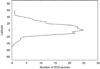 |
Fig. 6 Distribution of the location of the SO2 plumes as a function of latitude. |
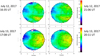 |
Fig. 7 Maps of the line depth ratio of a weak SO2 multiplet around 1345.1 cm−1 to the CO2 transition at 1345.22 cm−1. Data correspond to the July 12 and 13, 2017. It can be seen for each day that the SO2 plumes follow the four-day rotation, corresponding to an angle of 15° westward for a time difference of 4 h. In both cases, the intermediate maps taken between the first and last ones reproduce the SO2 pattern shown in this figure. The subsolar point is shown as a white dot. |
3.4 Distribution of the SO2 plumes as a function of local time
The same study was performed to estimate the probability of SO2 plume appearance as a function of local time (Figs. 10 and 11). Figure 10 shows that the dayside is most observed, with a maximum around noon, while there are few observations around midnight. Figure 11 shows the probability of SO2 plume appearance as a function of local time. A depletion seems to appear around noon, with a possible enhancement around the terminators. Between 22:00 and 02:30, the statistics are too low for the result to be significant. The SO2 depletion tentatively observed around noon (Fig. 11) is also observed on some of our maps; as shown in Fig. 7, the two maps are separated by 3 h in time and distinctly show a minimum of SO2 around the subsolar point and a maximum around the anti-solar region. The fact that the depletion around the subsolar point persists from July 12 to July 13, 2017, illustrates that this feature is not associated with the four-day rotation. We note that the configuration observed in July 2017 is also observed on December 23, 2016 (Fig. 4).
A possible explanation for this depletion might be a suppression of the cloud level convection, which could inhibit transport through the cloud layer, as suggested by Imamura et al. (2018). Other possible explanations might be a photochemical process, as suggested by the subsolar depletion, and/or a dynamical wave pattern. We could also wonder if the SO2 variation as a function of the local time might be the effect of a subsolar–anti-solar circulation. However, this seems unlikely, since this circulation is typically observed at higher altitudes, around 90 km (Lellouch et al. 2008), while the four-day super-rotation dominates at the cloudtop probed at 7.4 μm; we have seen that this super-rotation is actually observed on some SO2 plumes on atimescale of a few hours (E16).
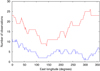 |
Fig. 8 Summation of all longitudes observed by TEXES over the 2012–2018 period, using the 34 observations listed in Table 1 (red curve). Summation of all longitudes where a SO2 plume was present, using the same dataset (blue curve). |
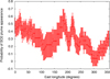 |
Fig. 9 Probability of SO2 appearance as a function of longitude, using the same dataset as in Table 1 and Fig. 8. The error bar is proportional to n−0.5, where n is the number of observations for which the longitude is observed (red curve in Fig. 8). |
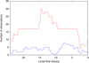 |
Fig. 10 Summation of all local time observed by TEXES over the 2012–2018 period, using the 34 observations listed in Table 1 (red curve). Summation of all local times for which a SO2 plume was present, using the same dataset (blue curve). |
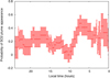 |
Fig. 11 Probability of SO2 appearance as a function of local time, using the data shown in Table 1 and Fig. 10. The error bar is proportional to n−0.5, where n is the number of observations for which the local time is observed (red curve in Fig. 10). |
4 Comparative analysis of the SO2 and H2O variations
4.1 HDOmaps in 2016 and 2017
Figure 12 shows examples of HDO maps recorded between January 2016 and July 2018, using the same observations as shown in Figs. 2–4. Figure 13 shows the HDO maps corresponding to the sequence of January 13–21, 2016. A difference should be noted with respect to the maps shownin E16 for the first half of this sequence. We realized in some cases that the terrestrial atmospheric transmission dominates the spectrum in such a way that the HDO retrieval is not reliable, and the HDO map should be excluded. This was the case for the HDO maps of October 5, 2012, July 7, 2014, and January 14, 2016, shown in our previous paper. In the present analysis, we limit the HDO analysis to the data showing little telluric contamination.
The maps shown in Figs. 12 and 13 confirm our earlier statements regarding the water distribution over the disk of Venus and its evolution as a function of time. The HDO maps are remarkably uniform over the Venus disk, showing no patchy feature comparable to the SO2 maps or any signature that could be associated with the latitude, longitude, or local time. In particular, we see no correlation or anti-correlation between the SO2 and HDO mixing ratios on a local scale. It is interesting to compare the SO2 and HDO maps recorded on July 13, 2017 (Figs. 4 and 12). The atmospherictransmission was especially good on that date, as shown in Fig. 2. While the SO2 distribution shows a factor of 4 variation between the anti-solar region (maximum) and subsolar (minimum) region, the HDO distribution is flat all over the disk down to the 15% level. Another example of the homogeneity of the HDO distribution is shown in Fig. 14, where HDO maps are presented for different local time ranges, on January 21, 2017 (evening terminator), and July 13, 2017 (morning terminator). The HDO map of July 12, 2017, is integrated over the four observations described in Table A.1. It can be seen that the fluctuations of the HDO vmr over the disk are below 10% for the morning and the evening configurations.
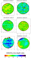 |
Fig. 12 Maps of the line depth ratio of the HDO transition at 1344.90 cm−1 to the CO2 transition at 1345.22 cm−1. Data are the same as in Figs. 2–4. The subsolar point is shown as a white dot. |
4.2 Long-term variations of SO2 and H2O from 2012 to 2017
Figure 15 shows the long-term variations of SO2 and H2 O over the whole TEXES dataset. As in our previous analysis, the SO2 and HDO volume mixing ratios are inferred from the SO2/CO2 and HDO/CO2 line depth ratios measured on the disk-integrated spectra corresponding to each observation; the SO2 mixing ratios are thus lower than the values listed in Table 1, which correspond to the maxima volume mixing ratios of the SO2 plumes. As mentioned above, the H2O mixing ratios are inferred with the assumption that the mesospheric value of D/H in Venus is 200 times the VSMOW (Fedorova et al. 2008).
In the case of SO2, unlike our previous analysis (E16), we limited our analysis to the 7.4 μm data. We note that the retrieval of the SO2 volume mixing ratio at 18.9 μm (already difficult for low abundances of SO2 because of the strong curvature of the continuum, see E16) becomes uncertain when the SO2 content is large because the SO2 and CO2 transitions overlap; this restriction applies to all data taken in 2016 and 2017. The analysis of the 18.9 μm SO2 data in 2016 and 2017 will be performed in a forthcoming publication. In the case of HDO, we disregarded the observations corresponding to a high terrestrial opacity. There seems to be a trend for H2 O to decrease as a function of time between 2016 and 2018, from about 1.2 ppmv in 2016 to 0.5 ppmv in 2018; similarly, there may be a long-term increase in the SO2 mixing ratio from 2014 (minimum value of 30 ppbv) to 2018 (maximum value of 600 ppbv). However, as mentioned in our earlier studies, we see no clear evidence for an anti-correlation in the long-term variability of SO2 and H2 O at the cloudtop.
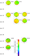 |
Fig. 13 Maps of the HDO/CO2 line depth ratio, using the HDO transition at 1344.90 cm−1, divided by the CO2 transition at 1345.22 cm−1, between January 13, 2016, and January 21, 2016. Data are the same as in Fig. 5. |
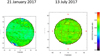 |
Fig. 14 Maps of the HDO/CO2 line depth ratio, using the HDO transition at 1344.90 cm−1 to the CO2 transition at 1345.22 cm−1, on January 21, 2017, and July 12, 2017. The subsolar point is shown as a white dot. |
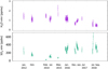 |
Fig. 15 Long-term variations of the H2O volume mixing ratio (top panel), inferred from the HDO measurements, and the SO2 volume mixing ratio (bottom panel), measured at the cloudtop using the TEXES data at 7.4 μm. |
5 Comparative analysis of TEXES results with Venus Express and Akatsuki space data
The time range covered by our dataset (2012–2017) overlaps with two sets of UV space data, the first recorded by Venus Express (2006–2015)and the second by Akatsuki (in operation since December 2016). In the UV range, the distribution of the SO2 gas above the cloudtop can be approximated using the 283 nm spectral feature, where the SO2 absorption is stronger than other agents (Pollack et al. 1980). We note that the UV radiation comes from a slightly higher level that the IR radiation, i.e., a few kilometers above the cloudtop.
5.1 Comparison of TEXES with Akatsuki/UVI
Figure 16 shows an example of the anti-correlation observed between the TEXES SO2 map (inferred from the ratio of absorption depths of SO2 and CO2) and the map of the UV (λ = 283 nm) albedo, as measured by the UV imager (UVI) on board Akatsuki on January 21, 2017. The observation time was 03:43–04:18 UT and 01:46 UT for TEXES and Akatsuki, respectively. The UV radiances measured by Akatuki UVI were corrected for the incident and emission angle dependences of reflection assuming the Lambert Lommel-Seeliger law (Lee et al. 2017), and projected on a disk map corresponding to the geometry observed from the Earth. It is clearly shown that the dark (low-albedo) regions on the UV map match the large SO2 regions in the TEXES data. The very good agreement (shown by a correlation factor of 0.89) between the two maps indicates that using imaging spectroscopy, in the UV at 283 nm and in the IR at 7.4 μm, provides equally good tracersof the SO2 abundance above the clouds. As a result, TEXES maps can be used to extrapolate the day side’s UV maps of Akatsuki to the night side.
This comparison was performed for nine datasets of Akatsuki and TEXES (observation time differences within a maximum of 6 h). The correlation plot is shown in Fig. 17. For this quantitative comparison, Akatsuki data were smoothed to the same spatial resolution as the TEXES observations. Very good anti-correlations are observed between Akatsuki UV albedo and TEXES SO2 maps on December 16 and 22, 2016, and on January 20–22, 2017, whereas some have no strong correlations. The reason might be that the 283 nm channel is sensitive to the SO2 band, but also possibly to the UV absorber which in some cases might have a different spatial distribution from that of SO2. Further analysis using radiative transfer calculations will be performed in a future work.
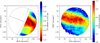 |
Fig. 16 Left panel: UV albedo map derived from the Akatsuki UVI data recorded on January 21, 2017, at 01:46 UT. Dashed lines represent the equator and the evening terminator. Right panel: TEXES map of the SO2 volume mixing ratio at the cloudtop, inferred from the SO2/CO2 line depth ratio at 7.4 μm on January 21, 2017, at 03:43–04:18 UT. |
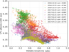 |
Fig. 17 Correlation between Akatsuki UV albedo at λ = 283 nm and TEXES SO2 maps. The label “corr” indicates the correlation factor for the comparison data. |
5.2 Comparison of TEXES with SPICAV aboard Venus Express
Between 2006 and 2015, the abundance of SO2 above the clouds was monitored by the UV spectrometer SPICAV aboard Venus Express, through the measurement of the 283 nm absorption band of SO2 (Marcq et al. 2013).SO2 maps were obtained as a function of time, latitude, longitude, and local time. Figure 18 shows a comparison of the SO2 volume mixing ratio observed by SPICAV above the clouds and the SO2 vmr recorded by TEXES at the cloudtop. A scaling factor was applied to the TEXES data to take into account the SO2 depletion above the clouds, according to a scale height of about 3 km: at the altitude of 70 km probed in the UV, the SO2 vmr is expected to be about 3 times lower than its value at the cloudtop. It can be seen that the agreement between the two datasets is satisfactory.
Figure 19 shows a comparison between the SO2 volume mixing ratioas a function of the local time, as seen by SPICAV aboard Venus Express between 2006 and 2015, and the probability of SO2 plume occurrence as seen by TEXES between 2012 and 2017. In both cases, a minimum seems to appear around noon. We note that the two quantities are not equivalent since the probability of occurrence of a SO2 plume derived from the TEXES data does not take into account the intensity of the plume. More data will be needed to confirm this trend.
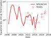 |
Fig. 18 Volume mixing ratio of SO2 at an altitude of 70 km, inferred from the SPICAV data. Superimposed: TEXES measurements of SO2 rescaled for an altitude of 70 km. |
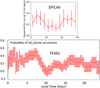 |
Fig. 19 Top panel: SO2 volume mixing ratio, as observed by SPICAV aboard Venus Express at an altitude of 70 km as a function of local time, including all data between 2006 and 2015. Bottom panel: probability of occurrence of an SO2 plume as a function of local time, including TEXES data between 2012 and 2018 (see Fig. 11). |
6 Conclusions
In this paper, we presented the data of our SO2 and HDO monitoring at the cloudtop of Venus using the TEXES instrument at 7.4 μm between January 2016 and September 2018. Then we used the whole TEXES dataset between 2012 and 2018 to analyze the behavior of the SO2 as a function of time, latitude, longitude, and local time. The main results of this study can be summarized as follows:
-
The SO2 maps at the cloudtop show a patchy distribution over the disk, while the HDO maps are very uniform.
-
The disk-integrated SO2 volume mixing ratio at the cloudtop shows variations of over a factor of 10 between 2012 and 2018, with a minimum in February 2014 (30 ppbv) and a maximum in July 2018 (600 ppbv). At the same time, the H2O volume mixing ratio (assuming a D/H of 200 × VSMOW in the Venus mesosphere, Fedorova et al. 2008) shows fewer variations, but a possible decrease from about 1.2 ppbv in 2016 to 0.5 ppbv in 2018.
-
The SO2 plumes are mostly concentrated around the equator, within the (30N–30S) latitude range.
-
The SO2 plume distribution as a function of longitude might indicate a depletion between 100E and 150E longitudes (corresponding to the region of Aphrodite Terra) and around 300E longitude; however, this trend remains to be confirmed with further observations.
-
The SO2 plume distribution as a function of local time seems to show a minimum occurrence around noon, with two possible maxima around the terminator. The depletion around 12:00, if confirmed, could be the signature of convection inhibition (Imamura et al. 2018), or photochemical processes associated with the incidence angle, or dynamical transport. Presently, the limited amount of data prevents us from drawing a firm conclusion on this phenomenon.
-
A very good agreement is observed between the SO2 measurements of TEXES and Akatsuki UVI regarding the local distribution of SO2 over the Venus disk. The comparison of TEXES with the UV data of SPICAV aboard Venus Express also shows a good agreement for the long-term variations of the SO2 intensity, and for the SO2 distribution as a function of local time. These results illustrate that the TEXES data can be used to extrapolate the UV data on SO2 over the night side.
It is interesting to note that theoretical models have predicted the possible occurrence of oscillations in the Venus atmosphere. Takagi et al. (2018) have modeled the latitude distribution of amplitude of the vertical wind associated with thermal tides with modes 1 (most dominant at any latitude), mode 2 (below 30N), mode 3 (at 30–40N) and mode 4 (at 30–70N). This means that mode 1 and mode 2 oscillations would be expected to be dominant below 30N. Further observations with TEXES, especially near inferior conjunctions and, whenever possible, coupled with Akatsuki campaigns, will hopefully allow us to better constrain the SO2 behavior at the cloudtop over the day and night sides.
Acknowledgements
T.E. and T.K.G. were visiting astronomers at the NASA Infrared Telescope Facility, which is operated by the University of Hawaii under Cooperative Agreement no. NNX-08AE38A with the National Aeronautics and Space Administration, Science Mission Directorate, Planetary Astronomy Program. We wish to thank the IRTF staff for the support of the TEXES observations. This work was supported by the Programme National de Planétologie (PNP) of CNRS/INSU, co-funded by CNES. T.K.G. acknowledges the support of NASA Grant NNX14AG34G. E.M. acknowledges support from ESA and CNES for the analysis of the SPICAV-UV data. T.E. and B.B. acknowledge support from CNRS. T.F. acknowledges support from UPMC. T.W. acknowledges support from the University of Versailles-Saint-Quentin and the European Commission Framework Program FP7 under Grant Agreement 606798 (Project EuroVenus).T.E. acknowledges support from the Jet Propulsion Laboratory as a Distinguished Visiting Scientist.
Appendix A Additional table
Summary of TEXES observations from January 2016 to September 2018.
References
- Belyaev, D. A., Montmessin, F., Bertaux, J.-L., et al. 2012, Icarus, 217, 740 [NASA ADS] [CrossRef] [Google Scholar]
- Bézard, B., & DeBergh, C. 2012, J. Geophys. Res., 112, E04S07 [Google Scholar]
- Crisp, D. 1986, Icarus, 67, 484 [NASA ADS] [CrossRef] [Google Scholar]
- Encrenaz, T., Greathouse, T. K., Richter, M. J., et al. 2008, Icarus, 179, 43 [NASA ADS] [CrossRef] [Google Scholar]
- Encrenaz, T., Greathouse, T. K., Roe, H. et al. 2012, A&A, 543, A153 [NASA ADS] [CrossRef] [EDP Sciences] [Google Scholar]
- Encrenaz, T., Greathouse, T. K., Richter, M. J. et al. 2013, A&A, 559, A65 [NASA ADS] [CrossRef] [EDP Sciences] [Google Scholar]
- Encrenaz, T., Greathouse, T. K., Lefèvre, F. et al. 2015, A&A, 578, A127 [NASA ADS] [CrossRef] [EDP Sciences] [Google Scholar]
- Encrenaz, Greathouse, T. K., Richter, M. J. et al. 2016, A&A, 595, A74 [NASA ADS] [CrossRef] [EDP Sciences] [Google Scholar]
- Fedorova, A., Korablev, O., Vandaele, A.-C. et al. 2008, J. Geophys. Res., 113, E00B25 [CrossRef] [Google Scholar]
- Imamura, T., Miyamoto, M., Ando, H. et al. 2018, J. Geophys. Res., 123, 2151 [CrossRef] [Google Scholar]
- Krasnopolsky, V. A. 1986, Photochemistry of the Atmospheres of Mars and Venus (New York: Springer-Verlag [CrossRef] [Google Scholar]
- Krasnopolsky, V. A. 2007, Icarus, 191, 25 [NASA ADS] [CrossRef] [Google Scholar]
- Krasnopolsky, V. A. 2010, Icarus, 209, 314 [NASA ADS] [CrossRef] [Google Scholar]
- Lacy, J. H., Richter, M. J., Greathouse, T. K. et al. 2002, PASP, 114, 153 [NASA ADS] [CrossRef] [Google Scholar]
- Lee, Y. J., Yamazaki, A., Imamura, T., et al. 2017, AJ, 154, 44 [NASA ADS] [CrossRef] [Google Scholar]
- Lellouch, E., Paubert, G., Moreno, R., & Moullet, A. 2008, Planet Space Sci., 56, 1355 [NASA ADS] [CrossRef] [Google Scholar]
- Marcq, E., Bertaux, J.-L., Montmessin, F. et al. 2013, Nat. Geosci., 6, 25 [NASA ADS] [CrossRef] [Google Scholar]
- Marcq, E., Mills, F. P., Parckinson, C. P., Vandaele, A.-C. 2018, Space Sci. Rev., 214, 10 [NASA ADS] [CrossRef] [Google Scholar]
- Mills, F. P., Esposito, L. W., & Yung, Y. K. 2007, in Exploring Venus as a Terrestrial Planet, Geophysical Mongraph Series (New York: John Wiley & Sons), 176, 73 [Google Scholar]
- Pollack, J. B., Toon, O. B., Whitten, R. C. et al. 1980, J. Geophys. Res., 85, 8141 [NASA ADS] [CrossRef] [Google Scholar]
- Rohlfs, K., & Wilson, T. L. 2004 Tools for Radioastronomy, 4th edn. (Berlin: Springer) [Google Scholar]
- Sandor, B. J., Clancy, R.T., Moriartry-Schieven, G., & Mills, F. P. 2010, Icarus, 208, 49 [NASA ADS] [CrossRef] [Google Scholar]
- Sandor, B. J., Clancy, R.T., & Moriartry-Schieven, G. 2012, Icarus, 217, 839 [NASA ADS] [CrossRef] [Google Scholar]
- Takagi, M., Sugimoto, N., Ando, N., & Matsuda, Y. J. 2018, Geophys. Res., 123, 335 [NASA ADS] [CrossRef] [Google Scholar]
- Vandaele, A.-C., Korablev, O., Belyaev, D. et al. 2017, Icarus, 295, 16 [NASA ADS] [CrossRef] [Google Scholar]
- Zasova, L. V., Moroz, V I., Esposito, L., W., & Na, C. Y. 1993, Icarus, 105, 92 [NASA ADS] [CrossRef] [Google Scholar]
- Zhang, K., Liang, M. C., & Mills, F. P. 2012, Icarus, 217, 714 [NASA ADS] [CrossRef] [Google Scholar]
All Tables
Summary of TEXES observations used for the analysis of the SO2 plumes (2012–2018).
All Figures
|
Fig. 1 Geometrical configurations of the disk of Venus during the six TEXES runs of 2016, 2017, and 2018. The terminator is indicated with a black line and the subsolar point with a black dot. The January 2016 and July 2017 runs correspond to the morning terminator; the four other runs correspond to the evening terminator. |
| In the text | |
|
Fig. 2 Examples of disk-integrated spectra of Venus between 1344.8 and 1345.4 cm−1 (7.4 μm) recorded between January 2016 and September 2018. |
| In the text | |
|
Fig. 3 Examples of maps of the line depth of the weak CO2 transition at 1345.22 cm−1 (7.4 μm), corresponding to the observations shown in Fig. 2. The scale is the same for the four maps. The subsolar point is shown as a white dot. |
| In the text | |
|
Fig. 4 Maps of the line depth ratio of a weak SO2 multiplet (around 1345.1 cm−1) to the CO2 transition at 1345.22 cm−1. The data are the same as in Figs. 2 and 3. The subsolar point is shown as a white dot. The scale is not the same for the six maps; the maximum SO2 abundance is observed in July 2018. |
| In the text | |
|
Fig. 5 Maps of the SO2/CO2 line depth ratio, using SO2 multiplets (around 1345.1 and 1345.3 cm−1) divided by the CO2 transition at 1345.22 cm−1, between January 13, 2016, and January 21, 2016. The subsolar point is shown as a white dot. |
| In the text | |
|
Fig. 6 Distribution of the location of the SO2 plumes as a function of latitude. |
| In the text | |
|
Fig. 7 Maps of the line depth ratio of a weak SO2 multiplet around 1345.1 cm−1 to the CO2 transition at 1345.22 cm−1. Data correspond to the July 12 and 13, 2017. It can be seen for each day that the SO2 plumes follow the four-day rotation, corresponding to an angle of 15° westward for a time difference of 4 h. In both cases, the intermediate maps taken between the first and last ones reproduce the SO2 pattern shown in this figure. The subsolar point is shown as a white dot. |
| In the text | |
|
Fig. 8 Summation of all longitudes observed by TEXES over the 2012–2018 period, using the 34 observations listed in Table 1 (red curve). Summation of all longitudes where a SO2 plume was present, using the same dataset (blue curve). |
| In the text | |
|
Fig. 9 Probability of SO2 appearance as a function of longitude, using the same dataset as in Table 1 and Fig. 8. The error bar is proportional to n−0.5, where n is the number of observations for which the longitude is observed (red curve in Fig. 8). |
| In the text | |
|
Fig. 10 Summation of all local time observed by TEXES over the 2012–2018 period, using the 34 observations listed in Table 1 (red curve). Summation of all local times for which a SO2 plume was present, using the same dataset (blue curve). |
| In the text | |
|
Fig. 11 Probability of SO2 appearance as a function of local time, using the data shown in Table 1 and Fig. 10. The error bar is proportional to n−0.5, where n is the number of observations for which the local time is observed (red curve in Fig. 10). |
| In the text | |
|
Fig. 12 Maps of the line depth ratio of the HDO transition at 1344.90 cm−1 to the CO2 transition at 1345.22 cm−1. Data are the same as in Figs. 2–4. The subsolar point is shown as a white dot. |
| In the text | |
|
Fig. 13 Maps of the HDO/CO2 line depth ratio, using the HDO transition at 1344.90 cm−1, divided by the CO2 transition at 1345.22 cm−1, between January 13, 2016, and January 21, 2016. Data are the same as in Fig. 5. |
| In the text | |
|
Fig. 14 Maps of the HDO/CO2 line depth ratio, using the HDO transition at 1344.90 cm−1 to the CO2 transition at 1345.22 cm−1, on January 21, 2017, and July 12, 2017. The subsolar point is shown as a white dot. |
| In the text | |
|
Fig. 15 Long-term variations of the H2O volume mixing ratio (top panel), inferred from the HDO measurements, and the SO2 volume mixing ratio (bottom panel), measured at the cloudtop using the TEXES data at 7.4 μm. |
| In the text | |
|
Fig. 16 Left panel: UV albedo map derived from the Akatsuki UVI data recorded on January 21, 2017, at 01:46 UT. Dashed lines represent the equator and the evening terminator. Right panel: TEXES map of the SO2 volume mixing ratio at the cloudtop, inferred from the SO2/CO2 line depth ratio at 7.4 μm on January 21, 2017, at 03:43–04:18 UT. |
| In the text | |
|
Fig. 17 Correlation between Akatsuki UV albedo at λ = 283 nm and TEXES SO2 maps. The label “corr” indicates the correlation factor for the comparison data. |
| In the text | |
|
Fig. 18 Volume mixing ratio of SO2 at an altitude of 70 km, inferred from the SPICAV data. Superimposed: TEXES measurements of SO2 rescaled for an altitude of 70 km. |
| In the text | |
|
Fig. 19 Top panel: SO2 volume mixing ratio, as observed by SPICAV aboard Venus Express at an altitude of 70 km as a function of local time, including all data between 2006 and 2015. Bottom panel: probability of occurrence of an SO2 plume as a function of local time, including TEXES data between 2012 and 2018 (see Fig. 11). |
| In the text | |
Current usage metrics show cumulative count of Article Views (full-text article views including HTML views, PDF and ePub downloads, according to the available data) and Abstracts Views on Vision4Press platform.
Data correspond to usage on the plateform after 2015. The current usage metrics is available 48-96 hours after online publication and is updated daily on week days.
Initial download of the metrics may take a while.