| Issue |
A&A
Volume 623, March 2019
|
|
|---|---|---|
| Article Number | A20 | |
| Number of page(s) | 22 | |
| Section | The Sun | |
| DOI | https://doi.org/10.1051/0004-6361/201732427 | |
| Published online | 26 February 2019 | |
Non-thermal hydrogen Lyman line and continuum emission in solar flares generated by electron beams
1
Northumbria University, Department of Mathematics, Physics and Electrical Engineering, 2 Ellison Pl, Newcastle upon Tyne NE1 8ST, UK
2
Institute for Solar Physics, Dept. of Astronomy, Stockholm University, Albanova University Center, 10691 Stockholm, Sweden
e-mail: malcolm.druett@astro.su.se
Received:
6
December
2017
Accepted:
13
January
2019
Aims. Hydrogen Lyman continuum emission is greatly enhanced in the impulsive kernels of solar flares, with observations of Lyman lines showing impulsive brightening and both red and blue wing asymmetries, based on the images with low spatial resolution. A spate of proposed instruments will study Lyman emission in more detail from bright, impulsive flare kernels. In support of new instrumentation we aim to apply an improved interpretation of Lyman emission with the hydrodynamic radiative code, HYDRO2GEN, which has already successfully explained Hα emission with large redshifts and sources of white light emission in solar flares. The simulations can interpret the existing observations and propose observations in the forthcoming missions.
Methods. A flaring atmosphere is considered to be produced by a 1D hydrodynamic response to injection of an electron beam, defining depth variations of electron and ion kinetic temperatures, densities, and macro-velocities. Radiative responses in this flaring atmosphere affected by the beams with different parameters are simulated using a fully non-local thermodynamic equilibrium (NLTE) approach for a five-level plus continuum model hydrogen atom with excitation and ionisation by spontaneous, external, and internal diffusive radiation, and by inelastic collisions with thermal and beam electrons. Integral radiative transfer equations for all optically thick transitions are solved using the L2 approximation simultaneously with steady state equations.
Results. During a beam injection in the impulsive phase there is a large increase of collisional ionisation and excitation by non-thermal electrons that strongly (by orders of magnitude) increases excitation and the ionisation degree of hydrogen atoms from all atomic levels. These non-thermal collisions combined with plasma heating caused by beam electrons lead to an increase in Lyman line and continuum radiation, which is highly optically thick. During a beam injection phase the Lyman continuum emission is greatly enhanced in a large range of wavelengths resulting in a flattened distribution of Lyman continuum over wavelengths. After the beam is switched off, Lyman continuum emission, because of its large opacity, sustains, for a very long time, the high ionisation degree of the flaring plasma gained during the beam injection. This leads to a long enhancement of hydrogen ionisation, occurrence of white light flares, and an increase of Lyman line emission in cores and wings, whose shapes are moved closer to those from complete redistribution (CRD) in frequencies, and away from the partial ones (PRD) derived in the non-flaring atmospheres. In addition, Lyman line profiles can reflect macro-motions of a flaring atmosphere caused by downward hydrodynamic shocks produced in response to the beam injection reflected in the enhancements of Ly-line red wing emission. These redshifted Ly-line profiles are often followed by the enhancement of Ly-line blue wing emission caused by the chromospheric evaporation. The ratio of the integrated intensities in the Lyα and Lyβ lines is lower for more powerful flares and agrees with reported values from observations, except in the impulsive phase in flaring kernels which were not resolved in previous observations, in which the ratio is even lower. These results can help observers to design the future observations in Lyman lines and continuum emission in flaring atmospheres.
Key words: Sun: flares / Sun: transition region / Sun: chromosphere / Sun: UV radiation / radiation mechanisms: non-thermal / line: profiles
© ESO 2019
1. Introduction
Advances in the observations of Lyman lines and continua are necessarily linked to the space-based missions capable of observing ultra-voilet (UV) emission. In 1953, detection of the Lyman-alpha (Lyα) line was reported in the spectrum of the Sun from balloon and rocket missions (Pietenpol et al. 1953; Byram et al. 1953). Soon after, observations of the OSO I satellite revealed the increases in Lyα intensity associated with solar flares (Hallam 1964). The earliest qualitative description of Lyman line observations during solar flares was provided using the observations from OSO III by Hall (1971) who reported enhancements of Lyα line emission as a percentage of the full-disc intensity, and derived a rise time of around 2.4 min and a decay time of around 4.4 min in the net Lyman emission intensity from the Sun.
In the 1970s, observations with higher spatial resolution reported brightenings of Lyα in the transient flare kernels combined with a great enhancement of the Lyman continuum and lines. These enhancements were associated with X-ray emission and surrounding Hα emission (Wood et al. 1972; Wood & Noyes 1972; Křivsky & Kurochka 1974; Machado & Noyes 1978) reflecting the impulsive and gradual components of a flare emission (Kelly & Rense 1972).
Spectral information about the Lyα line in the Sun became available in the 1980s. The first complete Lyα line spectra in flares from full-disc observations of the Sun with low temporal cadence were published by Canfield & van Hoosier (1980). The observed profiles show the line core with strong self-absorption, indicating large opacities throughout the flare and only slightly asymmetric wing intensities, with greater excess in the red wing before the flare maxima followed by a greater excess in the blue wing after the flare maxima. Lemaire et al. (1984) reported simultaneous spectrographic observations of many chromospheric lines during a flare, including Lyα and Lyβ measured with the OSO-8 satellite. The Lyα and Lyβ lines have emission profiles and both show the impulsive peaks rising for around 60 s and decaying for around 200 s, with the increased wing and core emission (Lemaire et al. 1984).
The practice of using full-disc images for Lyman line profile observations has persisted to the present day (MEGS-B instrument of the Extreme ultra-violet Variability Experiment, EVE (Woods et al. 2012), on board the Solar Dynamics Observatory, SDO (Pesnell et al. 2012)). Doppler velocities have been calculated from Lyβ − ϵ emission during the impulsive phase of solar flares from full-disc spectral observations (Sun-as-a-star observations; Brown et al. 2016). Flow speeds varying from 10 km s−1 to 60 km s−1 were derived from the similar observations depending on the line-fitting technique used, and whether the full disc intensity profiles or the quiet Sun subtracted intensity profiles were used. The line emission in these observations is the net emission from a variety of solar features: impulsive flare kernels, bright ribbons, and the surrounding active region. Therefore, one can interpret the flow speeds stated in Brown et al. (2016) as relating to the net active region emission and resulting from the techniques employed, rather than as indications of flow speeds in the flare foot-points.
The early radiative simulations using semi-empirical thermal response models of solar flares (Machado & Emslie 1979; Machado et al. 1980) could fit the observed emission from the Lα line only in the presence of a temperature plateau around the depths of hydrogen ionisation temperature. Furthermore, in order to match the observed Lyα emission intensities, this emission is required to be formed in the depths with rather high thermal electron densities of 3 × 10¹² − 3 × 1013 cm−3 (Machado & Emslie 1979). The ratio of the Lyα line intensity to the Lyβ line one was found to reduce from around 85 in the quiet Sun, to 35 in active regions, and to between 12 and 28 during solar flares (Basri et al. 1979; Machado et al. 1980). However, these models produced discrepancies for the emission at lower temperatures, such as Hα, and concluded that radiative losses from metal lines of Ca and Mg could also be important.
Zirin (1978), Canfield & van Hoosier (1980), Canfield et al. (1981) studied the ratio of the integrated intensities of hydrogen Lyα and Hα lines during solar flares. They found that the intensities of emission in these two lines were generally correlated and their ratio was approximately equal to unity. The authors had anticipated a greater increase of Lyman line emission, relative to the Hα line. It was inferred from their observations that a weakness of the Lyα line is due to photon trapping as a result of high optical depth. The authors concluded that a relative stability of the ratio in the emission from these lines is due to their joint roles in the cooling of the plasma. Hence, it was established that Lyman alpha (Lyα), the brightest line in the UV spectrum of the Sun with or without flares, and all other Lyman lines, are highly optically thick.
Moreover, Machado et al. (1980) demonstrated that Lyman continuum emission is a strong contributor to energy losses from flaring atmospheres, confirming that Lyman continuum emission is highly optically thick in the chromosphere. Morozhenko & Zharkova (1982), Zharkova (1983, 1984a) revealed that radiative transfer in Lyman continuum and its interaction with the radiation from all Lyman lines and other continua are very important for defining the ionisation balance of hydrogen atoms in solar atmospheres. Therefore, investigation of radiative transfer in Lyman lines and continuum is shown to be important for understanding the mechanisms of excitation and ionisation of hydrogen atoms throughout a flaring atmosphere.
High-cadence images have become available from the instruments using broadband filters, such as the transition region and coronal explorer, (TRACE), GOES/EUVS-E and PROBA2/LYRA. Rubio da Costa (Rubio da Costa et al. 2009, 2010, 2012) compared observations from high-cadence images with the results from their simulations using RADYN. They found that the integrated Lyα intensities produced in the simulations were higher than in the observations, and concluded that the code was better suited to modelling emission from Balmer lines. They also found that Lyα flare intensities are only weakly effected by the flux of the electron beam causing that flare, with the total intensity of each line varying by only a factor of two for beam fluxes varying over two orders of magnitude. However, this result is different from the pattern of simulated Lyα intensities published for the F10 and F11 flares of Allred et al. (2005).
More recently, Milligan & Chamberlin (2016) have shown that the inferences drawn from line and continuum enhancements in Lyman emission using broadband filters may be anomalous, resulting from the enhancements in the other lines and continuous emission captured by the broadband filter. For example, EVE Lyα light curves (using a broadband filter) show a rise time of tens of minutes at flare onset where other lines show a rapid increase (Hα, Lyβ, Lyman continuum). Alternatively, spectrally resolved flare observations of the same event by the Solar Stellar Irradiance Comparison Experiment (SOLSTICE) on-board the SOlar Radiation and Climate Experiment (SORCE) show a well defined peak in Lyα emission during the impulsive phase.
Several Lyman continuum spectra were reported from the late 1970s by Machado & Noyes (1978), Machado et al. (1980), with thermal (Avrett et al. 1986) and non-thermal (Zharkova & Kobylinskii 1993) flare models produced to interpret the spectra soon after. Sun-as-a-star continuum observations near the Lyman continuum head wavelength (910 Å) using the SUMER (Solar Ultraviolet Emission of Emitted Radiation) on-board SOHO (SOlar and Heliospheric Observatory), show a relative signal increase of 70%. Accounting for the area of the flare region, a local increase of the irradiance of the Lyman continuum is estimated to be a factor of several thousands, and this increase is sustained for a long time after the impulsive phase (Lemaire et al. 2004).
In general, the Lyman series has been remarkably underused in the studies of the solar atmosphere due to a lack of high-resolution imaging and spectroscopic instruments available. This state may be remedied by the spate of recently proposed instruments including the Extreme Ultraviolet Imager (EUI) and the Spectral Imaging of the Coronal Environment (SPICE) instrument aboard the Solar Orbiter (SO), the Chromospheric Lyman-Alpha SpectroPolarimeter (CLASP), the Lyman Alpha Spicule Observatory (LASO), and the Lyman-α Solar Telescope (LST) for the ASO-S mission (Li et al. 2016). Observations from this new generation of the instruments will provide high-resolution imaging of Lyman lines.
Before the advent of these instruments, it is important to study emission in the Lyman lines and continuum in the conditions relevant to solar flares affected by electron beams because this will help to produce better potential diagnostics of flaring atmospheres from the future Lyman observations. The HYDRO2GEN code offers one such opportunity as it considers fully NLTE (departures from local thermodynamic equilibrium, LTE) radiative transfer in the Lyman continuum and takes into account excitation and ionisation of hydrogen atoms by beam electrons from all excited states (Druett & Zharkova 2018). The models using this code have provided the successful interpretation of Hα line profiles with large red-wing enhancements observed during flare onsets (Druett et al. 2017), as well as the heights and intensities of white light signatures resulting from the hydrogen Paschen continuum emission in the impulsive flare kernels (Druett & Zharkova 2018; Battaglia & Kontar 2011, 2012; Martínez Oliveros et al. 2012; Krucker et al. 2015).
In the current paper we extend this model to simulation of the emission in Lyman lines and continuum, and probe these simulations with the existing observations. In addition, we attempt to predict possible features that could be observed in Lyman series using the next generation of the satellite payloads. A brief description of the hydrodynamic and radiative model is given in Sect. 2, the results of the simulations, and comparisons with observations, are described in Sect. 3, and the conclusions are drawn in Sect. 4.
2. Physical conditions and radiative model
For the physical conditions let us use the hydrodynamic models from Zharkova & Zharkov (2007) of flaring atmospheres heated by beam electrons with the initial energy fluxes described by the numbers in the model names (F10 - 1010, F11 - 1011 and F12 - 1012 erg cm−2 s−1). The hydrodynamic model considers two energy equations for electron and ion components, momentum, and continuity equations to describe the ambient plasma response to heating by beam electrons (Somov et al. 1981; Zharkova & Zharkov 2007) using a Lagrangian coordinate ξ. The plasma is heated by beam electrons injected from the top of the atmosphere and cooled off by radiative losses in the corona and chromosphere. The quiet Sun (QS) chromosphere is assumed to have a hydrostatic density distribution and a constant temperature of 6700°K (see details in Zharkova & Zharkov 2007; Druett et al. 2017, and references therein). This is different from the hydrodynamic models of Allred et al. (2005), that build the initial conditions for a flaring atmosphere already containing the quiet sun corona by starting from semi-empirical models for the chromosphere, derived from calcium emission (Carlsson & Stein 1997), and adding the transition region and corona with the apex held at a fixed temperature of 1 MK, with the atmosphere being relaxed to a state of hydrostatic and energetic equilibrium. Then, to this composite atmosphere, the heating is applied by beam electrons with higher cutoff energies, effectively reducing the magnitude of heating at the coronal levels, since higher energy (> 35 keV) electrons deposit the bulk of their energy at the chromospheric level.
In our hydrodynamic model the beam electrons with power-law energy distributions are injected at the top of the quiet Sun chromosphere (column depth of 1017 cm−2), precipitate down to the lower photosphere (column depth of 1023 cm−2), and form a flaring atmosphere with its own corona, transition region, and chromosphere/photosphere. Electron densities and heating functions at given column depths are found from the solutions of a continuity equation (Syrovatskii & Shmeleva 1972) assuming that the beam electrons heat the ambient plasma in Coulomb collisions with ambient electrons, ions, and neutral atoms. At the start of the simulation electron beams with spectral indices, γ, are injected for 10 s from the top of the atmosphere with triangular time profiles in energy fluxes (linearly increasing and decreasing, peaking at 5 s). The initial and boundary conditions are the same as described by Somov et al. (1981; see their Eqs. (5)–(12)).
In this study we utilise heating functions generated by power-law electron beams precipitating into a flaring atmosphere and heating it in Coulomb collisions (Syrovatskii & Shmeleva 1972; Dobranskis & Zharkova 2015). The lower cutoff energy of these beams is accepted to be 10 keV, which is equal to the lowest energy in a power-law part of the energy spectra of electrons accelerated in reconnecting current sheets (Zharkova & Gordovskyy 2005; Zharkova et al. 2005; Zharkova & Agapitov 2009) obtained for realistic magnetic field topologies of current sheets derived from magneto-hydrodynamic simulations (Somov & Oreshina 2000). This cutoff is lower than the one of 37 keV used in Allred et al. (2005) leading to a reduction of their heating in general, and to a shift to deeper chromospheric levels of the depth of maximal heating in particular. However, smaller cutoff energies were used in the updated version of RADYN (Allred et al. 2015) with heating functions derived from the Fokker-Planck approach.
In the current hydrodynamic model the heating due to Ohmic losses is ignored. However, we must emphasise that during a steady injection of electron beams we still assume that there are returning beam electrons (return current), which are turned back to the top by the electric field induced by beam electrons (Siversky & Zharkova 2009; Dobranskis & Zharkova 2015). This allows us to keep the plasma volume neutral in flaring atmosphere, thereby supporting a steady beam injection and heating. The injection of power-law beam electrons causes a hydrodynamic response of the ambient plasma to energy deposition by power-law electron beams that generates a new flaring atmosphere with its own corona, chromosphere, and photosphere, which is shifted in a linear depth deeper into the atmosphere (Somov et al. 1981; Zharkova & Zharkov 2007, 2015) and solar interior (see Fig. 7 in Macrae et al. 2018).
HYDRO2GEN uses the radiative losses calculated for these physical hydrodynamic models as described in Kobylinskii & Zharkova (1996). That is to say, similarly to McClymont & Canfield (1983), the contribution to energy losses from the lower-temperature emission (< 20 000°K) is included for hydrogen line and continua emission to account for radiative losses at the chromosphere and photosphere (Kobylinskii & Zharkova 1996; Zharkova & Zharkov 2007). The losses from hydrogen are calculated in the first run of the radiative model affected by beams for each set of given parameters used in the simulations. The files are created storing radiative losses in all lines and continua for all times and depths and their resulting hydrogen losses.
The hydrogen losses are then added to the standard radiative cooling curve of Cox & Tucker (1969) in the corona, calculated for all the optically thin coronal lines (Somov et al. 1981). The model is then recalculated to obtain the updated physical parameters (T, n and V). After this first run we do not feedback the new findings of hydrogen emission found from the current radiative model at present. This is validated by the fact that the characteristic radiative time (10−3 − 10−2 s) is much lower that the characteristic hydrodynamic time (30 s) (Shmeleva & Syrovatskii 1973; Antiochos 1980).
The ionisation degree in the hydrodynamic part of the HYDRO2GEN model is defined by a modified Saha equation (Zharkova & Zharkov 2007) because its effect on plasma heating at lower chromosphere is defined by the parameter a (see formula (2) in Syrovatskii & Shmeleva 1972). Other radiative hydrodynamic models often feed back into a hydrodynamic part the ionisation degree from the NLTE radiative transfer codes. This approach aims to reproduce the effect of ionisation, or the ambient electron density, and increased heating of lower atmospheric levels lagging in a hydrodynamic response (Heinzel 1991; Abbett & Hawley 1999; Carlsson & Stein 2002; Kašparová et al. 2009). In HYDRO2GEN we consider the heating of hydrogen at all atmospheric levels, although the particle numbers of beam electrons reaching the lower atmospheric levels is more than five orders of magnitude lower than that at the top of the atmosphere (Zharkova & Kobylinskii 1993). Hence, any additional heating coming from the beam electron scattering on additional protons and electrons appearing from non-thermal hydrogen ionisation is reduced by the same magnitude and can be considered negligible for the hydrodynamic problem.
Moreover, many of these other radiative models use approximations either of a detailed balance in Lyman series or neglecting ionisation from the excited states of hydrogen. Such approximations would more significantly affect the accuracy of calculation of the ionisation degree compared with our approach. Therefore, in the current hydrodynamic simulations we kept our original approach with the modified Saha ionisation equation for hydrogen ionisation. We also use the radiative model including non-thermal ionisation and excitation from all the atomic levels as well as the exchange between the first and higher levels of hydrogen atom (Lyman series) for all five levels of the hydrogen atom.
The resulting electron temperatures T (°K), macro-velocities νm (km s−1), and densities n (cm−3) from the HYDRO2GEN models are shown in the top, middle, and bottom rows of Fig. 1, respectively, versus column depth ξ (cm−2). The atmospheric profiles are shown for the F10 and F12 models in the left and the right columns, respectively. For each plot, the initial atmosphere (t = 0 s) is shown by the black line, the atmospheres for the impulsive phase (t = 2, 4 s) are plotted by the red lines, and for the gradual phase (t = 15, 30, 60, 90 s) by the purple to blue lines. The times of the hydrodynamic responses shown in the Fig. 1 are selected to match the times used in the analysis of the line and continuum profiles (see Sect. 3). A full description of the response for each model is given in Druett & Zharkova (2018). In all the models, the column depths range from 1017 to 1023 cm−2; although the column depths shown in the plots in this paper are slightly truncated to 1022 cm−2 for a better resolution of the curves in the depths where the Lyman emission lines are formed.
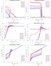 |
Fig. 1. Top row: temperatures (K), middle row: macro-velocities (km s−1), and bottom row: densities (cm−3) vs. column depth (cm−2) for the F10 (left col.) and F12 (right col.) atmospheric models. These profiles are shown for the initial atmosphere (t = 0 s, black line), impulsive phase atmosphere (t = 2, 4 s, red lines), and gradual phase (t = 15, 30, 60, 90 s, purple to blue lines) of the simulation in each figure. In each model the column depths run from 1017 to 1023 cm−2. |
These physical conditions are used as the input to the hydrogen radiative models described in detail by Druett & Zharkova (2018). Here we recapture the key point of this model. The radiative transfer problem is solved for five-level plus continuum model hydrogen atoms using joint steady state and integral radiative transfer equations for all optically thick transitions and steady state equations for optically thin transitions (11 equations in total; see Sect. 2 in Druett & Zharkova 2018). Similarly to Morozhenko & Zharkova (1982), Zharkova (1984a), Zharkova & Kobylinskii (1993), we consider radiative transfer in Lyman continuum with close exchanges from all Lyman line and other continua. For the solutions of radiative transfer integral equations used in our model, the L2 approach was applied (see for detail Druett & Zharkova 2018, and references therein) that provides a reasonable accuracy for source function throughout all the atmospheric depths.
All non-negligible radiative and collisional mechanisms of hydrogen ionisation and recombination, or excitation and de-excitation of all five levels and continua were considered including the diffusive and external (Lyman α, Balmer lines and Lyman continuum from the QS chromosphere) radiation and by collisions with thermal and beam electrons (Zharkova & Kobylinskii 1993). Excitation and ionisation rates by beam electrons are calculated for all the five atomic transitions and continua of the model hydrogen atom using the same cross-sections as for thermal electrons (see formulae in Zharkova & Kobylinskii 1993). The thermal and non-thermal collisional rates are compared by Zharkova & Kobylinskii (1989) that revealed a complete domination by a few orders of magnitude of non-thermal rates.
The simulations consider the NLTE radiative transfer in all the hydrogen transitions that are optically thick, which includes all Lyman and Balmer lines as well as the Lyman continuum, which governs the ionisation balance in the atmosphere (Druett & Zharkova 2018). In addition, the NLTE approach can include the Paschen α and β lines and the Bracket alpha line if their opacities are found to be higher than unity at any instant in a particular simulation. The macro-velocities of the plasma are included consistently in the calculations of the line absorption coefficients and the optical depth functions, the kernel functions of integral radiative transfer equations when integrating over wavelengths (see Eqs. (3), (5), (10) and (C.1) from Druett & Zharkova 2018) followed by their inclusion in the emergent intensities from lines, as presented in Sect. 3. We remind the reader that this defines the ionisation degree for a radiative transfer part of the code differently from the method used in a hydrodynamic part of the code (a modified Saha equation; Zharkova & Zharkov 2007) which is allowed because of different characteristic times for hydrodynamic and radiative processes discussed above (Shmeleva & Syrovatskii 1973).
The Lyman line cores are found to originate in the upper chromosphere and transition region. In order to resolve these regions more clearly, 20 additional depth points are included in our radiative model by interpolating the hydrodynamic model in the regions of the plasma with clearly monotonic variations in the plasma density, kinetic temperature, and macro-velocity. The upper chromosphere and transition region have a lower mass density, defining time-scales between the collisions of hydrogen atoms with the ambient electrons for Lyman transitions to be larger than the lifetime of an excited state in the atom. However, this effect is reduced in solar flares caused by the injection of a beam of energetic electrons leading to much higher collisional rates between beam electrons and hydrogen atoms (Zharkova & Kobylinskii 1993).
The HYDRO2GEN code has hitherto modelled all the hydrogen line emission under the assumption of complete redistribution of frequencies (CRD). However, under conditions of the quiet Sun chromosphere partial redistribution (PRD) in frequencies can affect the Lyman line wing emission due to coherent scattering (Basri et al. 1979; Hubeny & Lites 1995; Hubeny & Mihalas 2014). We believe this effect is less important during the injection of beam electrons whose collisional rates are a few orders of magnitudes higher than those of thermal electrons in the mid-chromosphere which are considered for a PRD treatment in the models of the quiet chromosphere. This is because the processes that are not coherent by their nature, such as collisions with ambient electrons and excitation directly from the beam electrons colliding with hydrogen atoms, are both increased by the presence of beams of electrons. Both these mechanisms will act to reduce the relative importance of coherent scattering.
Calculation shows (see Fig. 3 in Zharkova & Kobylinskii 1991) that additional ionisation by beam electrons increases the density of free electrons in the plasma by six orders of magnitude in the chromosphere where the Hα emission originates, and by two orders of magnitude in the upper chromosphere where Lyman emission is formed. Therefore, for the upper chromosphere with a density of, for example, 2 × 1012 cm−3 and ionisation without beam electrons of 10−2, this increase of ionisation degree by a factor of 100 will lead the ambient electron density to increase from 1010 to 1012 cm−3. We believe this reasoning implies that the incoherent, collisional approach becomes much more important for the formation of emission in Lyman line wings. Moreover, it was pointed out by Chluba & Sunyaev (2006, 2008, 2010) that redistribution in frequencies in the Lyα line transition occurs when the electrons bound to the hydrogen atoms are excited from the ground state and, rather than immediately returning back to ground state, reach higher levels and the continuum, from which they cascade down from one level to another before reaching the ground state again. This point was further developed by Roussel-Dupre (1983) investigating the theoretical condition of PRD, who found that for the wavelengths from the line centre of 0.5 Å < Δλ < 5 Å the Lyα line wing intensities are sensitive to the ambient electron density through their relationship to the quantity ne × T−1/2.
Hence, in the quiet Sun atmosphere where these wings are formed in the atmospheric levels where hydrogen is mostly neutral, scattering of the wing photons is close to coherent leading to a partial redistribution (PRD) in frequency of wing photons. However, in flares, as was shown for the Balmer and Pashen series (Zharkova & Kobylinskii 1991; Druett & Zharkova 2018), at these deep atmospheric levels there is a strong (by 5–6 orders of magnitude) increase of the hydrogen ionisation and excitation rates as a result of the beam electrons. This leads to the increase of impact excitation of the emission in the wings of Lyman line profiles, shifting them away from the PRD condition and towards the CRD condition. This happens because the required increase in the excitation rates of the hydrogen atom is supplied as a result of non-thermal collisions with beam electrons, increased thermal collisions at increased temperatures, and by a higher density of the ambient electrons caused by non-thermal ionisation.
By considering this point and the fact that the inclusion of PRD into the Lyman lines is very computationally expensive, in this paper the effects of PRD are mimicked by truncating the Lyman transition profiles at a set number of Doppler widths following the previous examples (Abbett & Hawley 1999; Allred et al. 2005; Carlsson & Leenaarts 2012). We choose this number to be ten, in order to reflect a reduction of the PRD effect due to the increased collisional rates caused by beam electrons.
Another important effect on the Lyman line profiles, in the presence of macro-velocities greater than the thermal Doppler velocities, is an angle-dependent PRD (Leenaarts et al. 2012). However, the current model does not yet include the modelling of these effects, and therefore some degree of caution should be exercised when interpreting the results for the Lyman lines.
3. Results of simulations
3.1. Lyman-α line profiles
The simulated Lyα profiles calculated for CRD and mimicked PRD (truncated at ten Doppler widths) of scattered photons are plotted versus a wavelength relative to the line centre in Fig. 2 during a beam injection phase from 1 s (a) to 4 s (d), respectively, for the F10 model (red lines), F11 model (green lines), and F12 model (blue lines). The Lyα line contribution functions (top row) and optical depths (bottom row) for the wavelength relative to the line centre (1216 Å) versus a column depth are shown in Fig. 3. In the top row of Fig. 3, logarithms of the Lyα contribution functions +1 are shown for the F10 model at 4 s (a) and for F12 model at 2 s after the beam onset (b). The colour scale runs from light (low contribution) to dark (high contribution), and the relevant plasma macro-velocity profiles are scaled to their resulting Doppler shifts, then plotted over the top of the contribution functions using a green line. The lower panels (c and d) display the logarithm of the optical depths +1 at the same times and for the same models. The optical depths are shown starting from a unity (blue) and increasing to an optical depth of ∼1010 in the line centre at the base of the model.
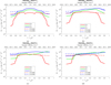 |
Fig. 2. Lyα line profiles calculated during the impulsive phase for mimicked PRD (solid lines) (see the text for details) and CRD (dashed lines). The profiles for the F10 model are shown with a red line, the F11 with a green line, and the F12 with blue for the times 1–4 s after beam injection in panels a to d. |
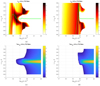 |
Fig. 3. Lyα line contribution functions (top row) and optical depths (bottom row) plotted for the wavelength relative to the line centre (1216 Å) versus the column depths during the beam injection. The contributions to the Lyα emission intensity are shown in panel a at 4 s in the F10 model and panel b at 2 s in the F12 model. The colour scale runs from light (low contribution) to dark (high contribution) in the logarithmic scale (contribution function + 1) panels, and the relevant plasma macro-velocity profiles are scaled to their resulting Doppler shifts, then plotted over the top of the contribution functions using a green line. Bottom panels: optical depths at the similar times. The logarithmic scale optical depths are shown starting from a value of τ = 1 (blue) and increasing to an optical depth of > 109 in the line centre at the base of the model (yellow). |
Non-thermal beam electrons injected into a flaring atmosphere have a dual effect on the ambient hydrogen plasma: (1) by heating via Coulomb elastic collisions and (2) by exciting and ionising hydrogen atoms through inelastic collisions. These two effects increase the abundances of hydrogen atoms with orbital electrons in levels 2–5 relative to the ground state and, as a result, lead to the growth of the hydrogen line source functions and contribution functions (Druett & Zharkova 2018); that is valid also for the Lyman line functions used in this paper. The contribution functions are calculated by taking the intensity integral over optical depths for a chosen line or continuum (see Eqs. (11) and (12) from Druett & Zharkova 2018), with the limits of integration defined by the optical depths at the top and bottom of the layer of the depth point under consideration. Therefore, the contribution functions are useful analysis tools because they show the contributions from a given depth point of the model to the total intensity of emission at the given wavelength.
The non-thermal collisions with powerful beam electrons remove the central reversals of the line cores of Lyα line during the first second after the beam onset (see the F11 and F12 Lyα line cores in Fig. 2a, in comparison to the core of the F10 model). The cores are wider and the wing emission is more increased in the models with stronger electron beams due to a greater collisional broadening (Fig. 2a). Also for the F11 and F12 models there are large Doppler shifts appearing in close red wings of the Lyα core emission 2 s after the beam onset (Fig. 2), which is earlier than those reported in Balmer lines (Druett & Zharkova 2018). These redshifts can be understood from the model atmospheres shown in Figs. 1d, e, and f, where one can see the downward-moving hydrodynamic shocks (positive macro-velocity) formed in the transition regions and upper chromospheres of the flare. These shocks are formed more swiftly for the hydrodynamic models with stronger beams, appearing in the formation region of the Lyman lines for the F11 and F12 models 2 s after the beam onset. The shock does not reach the formation region of the Balmer line cores until 3 s in the F11 and F12 models (see Fig. 7 of Druett & Zharkova 2018). While in the model F10 the shock is formed at a later time of 4 s after the beam onset and travels with a lower velocity while still significantly transforming the Lyα line cores and contribution functions (see Figs. 2d, 3a and c).
The contribution functions show that in the central wavelengths of Lyman lines, the emission intensity is sustained by a combination of the wing emission from the depths in which the core emission is Doppler-shifted to the red wing, and the core emission from the material at slightly deeper levels with the lower Doppler shifts (Fig. 2c, F11 and F12 models, Fig. 3b and d). By comparing the dashed line profiles (synthesised under the assumption of CRD) and solid line profiles (computed using the PRD mimicking, as described in Sect. 2) in Fig. 2, or by inspecting the contribution functions in Fig. 3 and relating the truncated wing emission shown here to the line profiles, one can see that the effects of PRD included in this modelling dramatically reduce the intensities in the wings of the Lyα line, whilst leaving the core emission largely unaffected. From the contribution functions we see that this PRD modelling potentially removes some contributions from deeper and cooler layers, with narrower Doppler widths at wavelengths more than 0.5 Å from the line centre. This mimicked PRD approach, however, does not suppress the highly enhanced red wing emission of the Lyα line in the impulsive phase, which is Doppler-shifted core emission and, thus, is not removed in the simulation by the truncation of the profiles at ten Doppler widths.
Mimicking the PRD line modelling by truncating wing emission in a CRD model aims to provide an approximation for radiative losses in Lyman lines, but detailed Lyman line profiles in the wings are not properly fully treated by this method and should be viewed with a measure of caution. Moreover, this exercise led us to the conclusion that the PRD approach may be less suitable for the simulations of Lyman line wing profiles in flaring atmospheres. In order to evaluate the effects of PRD on the wing profiles, we looked at the simulations by Roussel-Dupre (1983), who modelled the solar Lyα emission in wings for a number of non-flaring atmospheres and found that the Lyman line emission in the near-wing wavelengths in the range of Δλ = ±0.5 − 6 Å from the line centre are overestimated if using the assumption of CRD, and underestimated by a factor of four or more when using the PRD approach. As mentioned in Sect. 2, some authors (Roussel-Dupre 1983; Chluba & Sunyaev 2006, 2008, 2010) point out that in the atmospheres with the increased impact excitation and ionisation rates, the conditions of formation of Lyman line wings can be shifted from PRD closer to CRD. Since in the flaring atmospheres considered in this paper the impact excitation and ionisation by beam electrons dominates all other excitation and ionisation rates at all atmospheric depths (Zharkova & Kobylinskii 1991; Druett & Zharkova 2018), this allows us to suggest that the actual Lyman line wing intensities formed in flaring atmospheres affected by electron beams are moved closer to CRD, and away from PRD (see Figs. 2 and 4).
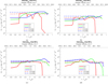 |
Fig. 4. Lyα line profiles calculated in the atmospheres after the electron beam is switched off for mimicked PRD (solid lines) and CRD (dashed lines). The profiles for the F10 model are shown with a red line, the F11 with a green line, and the F12 with blue for 15, 30, 60, and 90 s after beam injection in panels a to d, respectively. |
In Fig. 4 the Lyα line profiles are shown for four different times after the beam onset. The corresponding Lyα line contribution functions and optical depths during the beam injection are plotted in Fig. 5 at 30 s in the F10 model (panels a and c) and at 90 s in the F12 model (panels b and d). The axes and layout are the same as for Fig. 3.
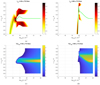 |
Fig. 5. Logarithm of the Lyα line contribution functions (top row) and optical depths (bottom row) after the beam injection. The logarithm of column depth is shown on the x-axis, and the wavelength relative to the line centre (1216 Å) is shown on the y-axis. The contributions to the Lyα emission intensity are shown in panel a at 30 s in the F10 model and panel b at 90 s in the F12 model. The colour scale runs from light (low contribution) to dark (high contribution) in the log(contribution function + 1) panels, and the relevant plasma macro-velocity profiles are scaled to their resulting Doppler shifts, and subsequently plotted over the top of the contribution functions using a green line. Bottom panels: logarithmic scale optical depths at similar times. The optical depths are shown starting from a value of τ = 1 (blue) and increasing to an optical depth of > 109 in the line centre at the base of the model (yellow). |
In order to understand these results, let us first discuss the general points related to the models used. Once the beam is switched off, a flaring atmosphere continues with a hydrodynamic response on a hydrodynamic timescale until its full cooling. The recombination rates of free electrons to hydrogen ions, or protons, is slower by a few orders of magnitude than the collisional ionisation rates of hydrogen atoms by beam electrons. This means that the ionisation degree of the hydrogen plasma gained during the beam injection can be maintained for a long period because of slow recombination rates (see Appendix A). Moreover, radiative transfer in the optically thick Lyman continuum keeps sustaining this ionisation degree of the hydrogen, because the diffusive radiation can only escape from the top layers of the atmosphere where the optical thickness is around unity (Morozhenko 1971, 1983; Morozhenko & Zharkova 1980, 1982; Zharkova 1983, 1984a,b) (see also Sect. 3.4).
The effect of this sustained ionisation maintained throughout extended atmospheric depths is that Lyα line profiles become highly broadened, while at the deeper atmospheric levels the maintained ionisation contributes to the increased wing emission. However, the wing emission has a lower optical depth than the radiation in the Lyα line core, and therefore radiation from the wings can escape, while the core emission from deeper levels is trapped due to the high optical thickness. This absorption creates a self-absorption in the line core with high double horns in the near wings combined with the small emission peak in the central wavelength due to the emission from the top layers of the chromosphere (Figs. 4a, b and 5). As after the beam offset the ambient electrons slowly recombine with protons and the plasma cools off, the emission intensities in the Lyα line core are decreased to the pre-flare level (Fig. 4).
Carlsson & Stein (2002) give a clear account of the relevant ionisation processes for hydrogen in the chromosphere and transition region in non-flaring conditions. Ionisation from the excited states of hydrogen is very important in the chromosphere, due to the lower-energy photons generated in, or penetrating to, these depths. Ionisation from the ground state becomes more important in the transition region where higher-energy photons are present. However, in a flare with non-thermal electron beams where energetic Lyman continuum emission is generated during the impulsive phase over a large range of depths by inelastic collisions with beam electrons, this balance is mainly governed by the trapped Lyman continuum radiation because of very slow hydrogen-electron recombination rates.
Lyman continuum radiation is optically thick, and escapes the flaring atmosphere only from the top layers where the optical thickness is about unity. Thus, the Lyman continuum radiation generated by beam electrons in the chromosphere is trapped in the atmosphere after the beam is turned off. This Lyman continuum radiation becomes rather intense and can be maintained in a flaring atmosphere for minutes in agreement with the observations reported in Machado & Noyes (1978). This trapped Lyman continuous emission sustains the high ionisation degree of hydrogen plasma that also helps to sustain emission of Balmer and Paschen continua (Druett & Zharkova 2018).
After the beam is switched off, temperatures of the flaring atmospheres decrease while the plasma still continues to up-flow from the greater column depths for another 100 s. The evidence of this up-flowing material is seen in the profiles of the Lyα line, derived from the flare transition region and upper chromosphere at later times of the simulation. For the plasma with temperatures < 50 000°K, which emits radiation in the Lyα line core, the up-flows occur at around 30 s for the F10 model. One can compare the column depth of 50 000°K plasma in Fig. 1a with the column depths showing the up-flows in Fig. 1b. These column depths match with the blueshifted core emission evident in the contribution function (Fig. 5a). The result of this up-flow is clearly seen in the blueshift of the Lyα line core in the F10 model at 30 s (Fig. 4b). This blueshift increases throughout the rest of the 100 s simulation.
For the models with stronger electron beams, the ambient plasma heating becomes much greater, and the flare transition region is shifted downward to greater column depths (Druett & Zharkova 2018). Thus, in the models with stronger beams the plasma up-flows occur from deeper column depths. As a result, Lyman line cores are formed in the regions which do not contain up-flows until later times in the simulation. A strong blueshift is seen in the Lyα line core at 90 s in the F12 model (Fig. 4d). This emission originates from the optically thin upper levels of the line formation region (see Figs. 5b and d, with column depths less than 1020 cm−2), which has a large spread of macro-velocities and, thus appears almost like a wing emission. The fact that this is the blue Doppler-shifted core emission and not wing emission can be proven from the contribution functions (Fig. 5d), as well as from the much greater emission in the blue wing of the Lyα line profile than in the red wing (Fig. 4d, blue line) calculated for the same model.
3.2. Profiles of other Lyman lines
The profiles for the Lyman beta (Lyβ) line simulated during the beam injection phase are shown in Figs. 6a–d, at 1–4 s after the beam onset, respectively. The Lyman γ (Lyγ) and δ (Lyδ) line profiles are found to be similar to those of Lyβ line (see Fig. 7). At the top of the flaring chromosphere, the emission in Lyβ line core wavelengths is significantly less optically thick than the emission of Lyα line core. Therefore, the Lyβ core emission can escape from this region from the first second of each simulation, forming the clear emission profiles with absolute intensities in the line core being lower than those in Lyα.
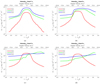 |
Fig. 6. Lyβ line profiles during the impulsive phase. The profiles for the F10 model are shown with a red line, the F11 with a green line, and the F12 with blue for 1, 2, 3, and 4 s after beam injection in panels a–d, respectively. |
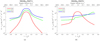 |
Fig. 7. Lyγ line profiles during the impulsive phase. The profiles for the F10 model are shown with a red line, the F11 with a green line, and the F12 with blue for 1 s after beam injection begins in panel a and after 4 s in panel b. These profiles are found to be similar to the Lyβ line profiles at the same times. |
There are also broader line cores seen again in the simulations for more powerful electron beams (see Fig. 6a). The core formation regions of higher lines in the Lyman series start at the same column depth as the Lyα lines, extending though to slightly greater column depths. Thus, after 2 s there is a significant enhancement seen in the red wing of the F11 and F12 models (see Fig. 6b) due to Doppler-shifted core emission from the downward motion of upper layers of the chromosphere. The Lyβ line intensity in the central wavelength is sustained by the emission from the deeper atmospheric layers, which have smaller associated Doppler-shifts at this time. In Figs. 6c and d calculated at 3 and 4 s after the beam onset, respectively, one can observe the emission peaks in the far red wings of the lines for the F11 and F12 models. This is because at these times the downward moving hydrodynamic shock expands to the core formation region. In the F10 model, the Doppler-shifted Lyβ core emission appears later than in the models with more powerful beams, and the extent of the Doppler shift is smaller (see Fig. 6d).
The profiles of Lyβ line occurring after the beam is switched off are shown in Figs. 8a–d, at 15, 30, 60, and 90 s into the simulation, respectively. In the F10 model, the Lyβ line core is much less broad than during the beam injection phase. Also, there is a blue asymmetry of the wing emission, clearly evident at 60 and 90 s due to the core emission coming from the very top of the line-formation region, in the transition region, in which plasma evaporation occurs. In fact, the blue asymmetries after the flare maximum are evident across the simulations of all Lyman lines. The ratio of the intensities of the Lyα and Lyβ lines is in agreement with the earlier observations reported for flares (Basri et al. 1979; Machado et al. 1980), and this is discussed in detail in Sect. 3.5.
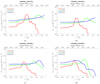 |
Fig. 8. Lyβ line profiles during the gradual phase. The profiles for the F10 model are shown with a red line, the F11 with a green line and the F12 with blue for 15, 30, 60, and 90 s after beam injection in panels a–d, respectively. |
3.3. Thermal and non-thermal Lyman line profiles
To elucidate the radiative effects of the beam electrons on the hydrogen line profiles revealed in the HYDRO2GEN simulations, we present a comparison of line profiles obtained from pure thermal and from thermal plus non-thermal simulations. In the thermal simulations, the hydrodynamic model used as input is the same as the models presented in Fig. 1, including the heating due to Coulomb collisions with beam electrons, but with the non-thermal rates of inelastic collisions between beam electrons and the ambient hydrogen set to zero. The resulting profiles are shown in Fig. 9; line profiles resulting from the thermal model are shown using the red lines, and non-thermal lines are shown in blue.
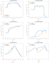 |
Fig. 9. Comparison of the emission in a thermal and a non-thermal flaring atmosphere. Thermal profiles are shown by the red lines, and non-thermal lines are shown in blue. Profiles are shown for the Lyα line after 4 s of the beam onset (panel a) and at 30 s (panel b) for the F10 flare, and after 4 s (panel c) 20 s (panel d) in the F11 flare model. The Lyβ line profiles are shown at 7 s of the simulation for the F10 flare (panel e). The Hα line profiles are shown at 40 s in the simulation for the F11 flare (panel f). |
The similarity of the cores of Lyman line profiles in the thermal and non-thermal models can be understood to result from their formation in the optically thin region at the very top of the chromosphere and in the transition region. In this region the thermal excitation rates dominate non-thermal ones, due to higher temperatures. The key differences between the profiles result from the excitation and ionisation caused by the non-thermal electron beam at greater column depths. This results in a large increase of close wing emission in Lyman lines for the non-thermal models compared to the thermal ones (Fig. 9, panels a–e). For lines formed at greater column depths, such as the Hα line, the core emission is more strongly affected by the beam electrons (Druett et al. 2017; Druett & Zharkova 2018). This is because the ionisation and excitation of hydrogen at the depths where these line cores form are dominated by the collisions with non-thermal electrons, whose excitation and ionization rates are much higher than those of thermal electrons or by radiation. It is this excitation that leads to much greater enhancements of the Hα line core intensities in the non-thermal flare model than in the thermal flare model (see the line cores in Fig. 9, panel f). The effects of non-thermal electrons on Hα core intensities are also discussed in Zharkova & Kobylinskii (1993), Fang et al. (1993), Abbett & Hawley (1999), Kašparová & Heinzel (2002), Allred et al. (2005) and associated papers. The highly optically thick Lyman emission is trapped in the mid-chromosphere in non-thermal cases, helping to sustain the levels of excitation and ionisation for a long time after the beam has stopped, as is evident from the enhanced wing emission of the profiles shown in panels b and d.
3.4. Simulations of Lyman continuum emission
The Lyman continuum is optically thick in the flaring chromosphere for all the hydrodynamic models (F10, F11, or F12). The simulated optical depths in the Lyman continuum head (911.8 Å) are shown in Fig. 10 as functions of column depth, and reach > 105 at all times at the base of each simulation. Moreover, the Lyman continuum becomes optically thick at the depths on the top of a flaring chromosphere. Therefore, Lyman continuum radiation escapes only from the very upper layers of the chromosphere in the models where its optical depth is approximately unity, thus governing the hydrogen ionisation in the underlying levels.
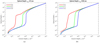 |
Fig. 10. Simulated optical depths in the Lyman continuum head wavelength. These are shown as functions of column depth during the beam injection phase at 5 s (panel a) and after the beam onset at 90 s of the simulation (panel b). The optical depths are calculated for the F10 (red line), F11 (green line), and F12 (blue line) models. |
The Lyman continuum emission profiles, during and after the beam injection, were calculated for the F10, F11, and F12 models, and are shown versus wavelengths in Fig. 11, as well as logarithms of the Lyman continuum contribution functions that show the heights from which the emission escapes as well as helping to explain the variations in the gradient of the Lyman continuum profile.
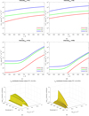 |
Fig. 11. Lyman continuum emission. Profiles are shown during the impulsive phase at 1 s (panel a) and 2 s (panel b) after the beam onset, and during the gradual phase after 15 s (panel c) and 90 s (panel d), calculated for the F10 (red line), F11 (green line), and F12 (blue line) models. Panels e and f: zoomed-in view of the logarithm of the Lyman continuum contribution functions for the F11 model after 2 and 15 s of the simulation, respectively. The contribution functions are plotted as functions of wavelength and column depth, demonstrating the column depths and, thus, the conditions responsible for the difference in gradient of the continuum emission during and after the beam injection phase of the flare. |
During an injection phase, beam electrons quickly (1 s) ionise the plasma, raising the intensity in the Lyman continuum at the same time as they heat the plasma to high temperatures. This process creates a low gradient of intensity variation away from the continuum head (Figs. 11a and b). The intensity of the emission scales with the intensity of an electron beam, and the intensity peaks co-temporally with the flux of the beam.
After the beam is switched off, the ionisation degree of hydrogen plasma is sustained by radiative transfer in the Lyman continuum and slow recombination of the ambient electrons with hydrogen atoms. Thus, the intensity of emission in the Lyman continuum head is reduced very slowly (Figs. 11c and d). However, the plasma also cools off, meaning that the recombinations are happening more frequently at lower temperatures than during the impulsive phase. Therefore, this leads to a steepening of the gradient of the Lyman continuum after the beam is switched off (Figs. 11c and d).
The ionisation degree is kept at the same level for a long time, leading to white light flares (Druett & Zharkova 2018). This reduction of the gradient of the Lyman continuum during the beam injection is consistent with the results reported for the F1 and F2 flare models of Ding & Schleicher (1997), when compared with their spectra from the quiet Sun emission. The continuum emission can be seen to originate from the column depths at the top of the chromosphere in Figs. 11e and f, where the decreasing temperature results in the steepening of the gradient of the continuum after the beam is switched off. The flattening of the spectrum at wavelengths below 700 Å, seen at later times in panels c and d of Fig. 11, results from the emission from high-temperature regions that have cooled sufficiently enough to allow some small amount of recombination to occur, which is the reason for low intensities of the Lyman continuum emission below 700 Å, comparable with the quiet Sun emission, even in the F12 model (Ding & Schleicher 1997).
3.5. Comparison with the Ly-α line observations and models
Radiative simulations in 1D models of flaring atmospheres can accurately reproduce the observed Balmer line profiles made with high spatial and temporal resolution in small flare kernels at the foot-points of reconnecting magnetic loops (Druett et al. 2017; Druett & Zharkova 2018). However, Lyman line profiles are generally obtained using low-resolution observations, or even images of the full solar disc, meaning that the Lyman emission is collected from these large areas and therefore is clearly not representative of that produced in a small flare kernel considered in the current models. Although these Lyman observations are not really comparable to those simulated from 1D models, some qualitative comparisons can still provide a valuable insight into the origin of Lyman series emission.
Firstly, the flare kernels are observed to be particularly bright in Lyman emission (Wood et al. 1972; Wood & Noyes 1972; Křivsky & Kurochka 1974; Machado & Noyes 1978). Secondly, these kernels are particularly associated with strongly asymmetric line profiles during the impulsive phase of the flare (Švestka et al. 1961; Ichimoto & Kurokawa 1984; Wuelser & Marti 1989; Li et al. 2015; Druett et al. 2017; Kowalski et al. 2017). Therefore, even with low-resolution flare observations, it may be possible for 1D models to reproduce the overall trends in the Lyman line asymmetries formed throughout a flare. Such attempts may, however, be confounded by the fact that flares generally show multiple beam injection locations with different onset times and temporal profiles or are located in active regions with other types of activities that can definitely complicate the interpretation.
Observed mild asymmetries in Lyα line profiles obtained from full-disc images of the Sun were reported by Canfield & van Hoosier (1980) with an excess in the red wing before the flare maximum followed by an excess in the blue wing after the flare maximum. These temporal variations of Lyα profiles are in agreement with our simulations for the Lyα flare kernel emission in the F10, F11, and F12 models in which we see greatly enhanced Lyman line wing emission. The simulations show the redshifted line profiles at the beginning of the impulsive phase lasting about 30 to 90 s, before switching to blueshifted profiles caused by evaporation of the chromospheric plasma back to the corona (Figs. 2, 4). The modelled Lyman line wings are found to be strongly affected by collisions with beam electrons and thermal electrons, whose density is increased by more than five orders of magnitude because of the increase of hydrogen ionisation (Zharkova & Kobylinskii 1991; Druett & Zharkova 2018). Therefore, in flaring atmospheres the angle dependent PRD of photons in frequencies (Leenaarts et al. 2012) is in competition with the strong impact excitation leading to the redistribution of photons in the line wings that push the wings closer to CRD (Roussel-Dupre 1983; Chluba & Sunyaev 2006, 2008, 2010).
This is evident from the observations of Lyman lines by Lemaire et al. (1984), which are in general agreement with the Lyman line emission simulated in our CRD models. Specifically, our models show clear impulsive peaks in integrated line intensities during the beam injection phase, which are also co-temporal with the increased Hα line wing emission produced by beam electrons in inelastic collisions with hydrogen atoms. In order to visualise these peaks occurring during the impulsive phase of beam injection, i.e. for the first ten seconds of the simulation, we present in Fig. 12 the integrated intensities of the Lyα line plotted on the Y-axis in logarithmic scale against the time (X-axis) after a beam onset for the F10 (red line), F11 (green line), and F12 (blue line) models simulated with HYDRO2GEN. The simulations clearly show strong intensity peaks in all the hydrodynamic models. This increase can be identified using the F10 model and Lyα line intensities where the line core stays well within a wavelength window of the simulation as shown in Figs. 2 and 4. Alternatively, the F12 model shows a dramatic decrease in Lyα intensity only a few seconds after the beam onset because the line core is shifted to the red wing outside the spectral window for simulated intensities (see Fig. 2).
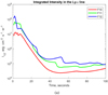 |
Fig. 12. Total intensities integrated across the wavelengths of the Lyα line in the F10 (red line), F11 (green line), and F12 (blue line) HYDRO2GEN model. |
A comparison of our simulations with the line profiles and macro-velocities derived from redshifted emission in the higher Lyman line observations reported by Brown et al. (2016) is particularly difficult because the reported macro-velocities are shown to be highly dependent on a method of measurements used. For example, in one flare the maximum Doppler shift calculated from the observations of the Lyβ line emission with the subtracted quiet Sun intensity profiles varies between 15 and 60 km s−1, depending on whether the Doppler shift is estimated using a Gaussian, a cross correlation function, or a weighted intensity method. Moreover, since the data use full disc intensities, even with the subtracted quiet Sun profiles the reported Doppler shifts relate to the average velocities over the whole active region, rather than the speeds in given flare kernels. We note that the Doppler shifts reported by Brown et al. (2016) are generally in line with those seen in the F10 model (±60 km s−1) and lower than the velocities seen in the F11 and F12 simulations. This could be a real reflection of the specific flaring events considered or could partially carry some limitations of the method of detection discussed above.
The high efficiency of energy losses from the Lyα line in semi-empirical thermal response models of solar flares suggested a temperature plateau around the hydrogen ionisation temperatures (Machado & Emslie 1979), but can be explained more simply in a non-thermal flare model with an injection of energetic electrons and additional hydrogen ionisation expanded over a wider range of atmospheric depths. The non-thermal ionisation and excitation by beam electrons in the chromosphere causes greatly enhanced emission in the near wings of the Lyα line during the beam-injection phase and for a sustained period after the beam is switched off (see Fig. 9), and simultaneously removes the discrepancies noted in the thermal semi-empirical models for emission at lower temperatures, such as Hα (Druett et al. 2017). Moreover, the results of the HYDRO2GEN simulations satisfy the conditions for plasma and ambient electron density in the range 3 × 10¹² − 3 × 1013 cm−3 that are required to explain the observed differential emission measures (Machado & Emslie 1979; Machado et al. 1980) at the column depths where the Lyman line and continuum emission is formed. It can be noted in the hydrodynamic models presented here (see the number densities in panels e and f of Fig. 1, at the top of the flaring chromospheres, where the ionisation degree of hydrogen is very high) that the Lyman line formation regions have plasma and electron densities reaching about 1013 cm−3, which is very close to the requirements imposed by Machado & Emslie (1979).
The HYDRO2GEN simulations show Lyman line formation regions over a slightly deeper and larger range of depths than those simulated in Machado et al. (1980), Avrett et al. (1986). However, it is important to emphasise that in the HYDRO2GEN simulations, lines are still found to be formed at the top of the flaring chromospheres, only with some additional radiation escaping in the wings from the upper middle chromosphere (see Figs. 3 and 5). This description is consistent with the radiative losses in the Lyman lines published in Kobylinskii & Zharkova (1996; see their Fig. 2a) for a predecessor of the current HYDRO2GEN model, which shows Lyman radiation dominating losses from hydrogen in a solar flare above the column depths of around 1019 cm−2 but becoming negligible from column depths greater than around 1020 − 1020.5 cm−2, where contributions from chromospheric lines become dominant.
The slightly deeper formation regions found in the HYDRO2GEN models compared to those of Machado et al. (1980), Avrett et al. (1986) result from a combination of factors. Firstly, Machado et al. (1980), Avrett et al. (1986) do not consider non-thermal excitation and ionisation by beam electrons, leading them to produce increased wing emission only deeper in the atmosphere. Secondly, they do not consider the effects of the Doppler shifts on the optical depths in lines, included in the HYDRO2GEN models, occurring due to plasma sweeping downward in the hydrodynamic shocks and upward in chromospheric evaporation. The Doppler shifting, beam sweeping, and the increase of wing emission due to non-thermal beam electrons will also act to increase in our models the depths and range of formation depths for other lines, similar to Balmer lines reported in the previous paper (Druett & Zharkova 2018). These other lines are still formed at greater depths than the Lyman lines in HYDRO2GEN models; the formation region of Hα in particular was discussed in Sect. 3.3. Paschen lines, which were shown to decrease their formation column depths in flares with strong beams (Druett & Zharkova 2018) are also still formed at depths much deeper than the Lyman lines, even in the case of the strongest flare models.
The reduction in the ratio of Lyα to Lyβ integrated intensities observed in flares when compared to active regions and the quiet Sun (Machado et al. 1980) can also be explained using the HYDRO2GEN non-thermal beam models of flares. The simulated flares more easily put the Lyβ line into emission than they do Lyα because the lower optical depths of the Lyβ line results in their core and wing formation regions extending to greater depths, where beam electrons effectively excite the electrons in hydrogen atoms and wing formation is further enhanced due to ionisation resulting from collisions between ambient hydrogen atoms and energetic beam electrons. In the HYDRO2GEN simulations, the ratio of the Lyα to Lyβ integrated line intensities after 40 s of the flare is 19.2 for the F10 model and 14.2 for the F12 flare model in agreement with the observed values of between 12 and 28 for scans of 3.8 min in duration during solar flares (Machado et al. 1980). These ratios remain within the observed parameters reported in Machado et al. (1980) beyond 20 s into the simulation, also exhibiting the reported pattern of lower ratios in simulations with greater fluxes of beam electron energy. In the beam-injection phase of the flare, in the foot-points where the beams are being injected we find that this ratio can decrease even further, reaching as low as 7 in the F12 flare. However these values could not be detected from the lower cadence (3.8 min scans), and lower-spatial-resolution (5″) observations available to Machado et al. (1980) at the time. Since the observations of Machado et al. (1980) were made using intensity integrated spectral windows, one should also exercise caution in their interpretation (Milligan & Chamberlin 2016).
3.6. Comparison with the observations of Lyman continuum enhancement
The quiet Sun emission intensities in the Lyman continuum head provided in the models of Ding & Schleicher (1997) are all in the range 102 − 103 erg cm−2 s−1 sr−1 Å−1. Lemaire et al. (2004) report impulsive enhancements of Lyman continuum emission at ∼900 Å in the bright flare kernels that are several thousand times greater than the background enhancements in the quiet Sun. The similar increase of intensity in the hydrogen Lyman continuum head (λ = 910 Å) is simulated by us during a beam injection for the F12 model (see Fig. 11b, blue line). This is more than 100 times higher than the Lyman continuum emission simulated at 90 s after a beam onset in the F10 model (see Fig. 11d, red line), which is again much greater than the emission from the quiet Sun.
The enhancements observed by Lemaire et al. (2004) are therefore shown to be consistent with the enhancement from ionisation of the ambient plasma by the non-thermal beam electrons through inelastic collisions, as shown in our models. Moreover, Table 2 of Lemaire et al. (2004) demonstrates that the ratio of enhancements in Lyman continuum emission observed in a flare compared to the quiet Sun levels is smaller at the wavelengths close to the continuum head (910 Å) than at slightly lower wavelengths (890 Å). This is consistent with the explanation provided using the HYDRO2GEN model for flattening of the Lyman continuum spectral profile during a beam injection phase (Fig. 11), which we suggest to result from higher ionisation degrees and ionisation temperatures caused by energetic beam electrons injected into a flaring atmosphere.
The intensities of emission in the Lyman continuum heads in each model are found to only drop by a factor of approximately ten during the 80 s period after the beam is switched off (see Fig. 11d). This decay rate agrees well with reports of the particularly bright impulsive enhancements above the general Lyman continuum increase in flaring atmospheres, lasting about 2 min in small kernels (Machado & Noyes 1978). The slow decay of the impulsive brightening is the result of radiative transfer in the frequencies of the Lyman continuum, which is highly optically thick, thus trapping the radiation below the column depths with opacities of the order of unity, and sustaining the ionisation degree throughout all the depths of the model.
The Lyman continuum intensity profiles of the F10, F11, and F12 HYDRO2GEN models during beam injection (Fig. 11) are comparable to those in F1, F2, and F3 models presented in Avrett et al. (1986), respectively. In the beam-injection phase the Lyman continuum profiles form at higher temperatures due to the beam heating at the top of the atmosphere, which matches to some extent the temperature increases used in the similar regions for the semi-empirical atmospheres used in Avrett et al. (1986).
In the HYDRO2GEN models, Lyman continuum emission only escapes from the optically thinner upper layers of the chromosphere in a narrow band with an optical depth of ∼1 (see the Lyman continuum contribution functions in panels e and f of Fig. 11 and compare these with the losses in Fig. 2 of Kobylinskii & Zharkova 1996). This description is in general agreement with the findings of Machado et al. (1980) Avrett et al. (1986) who predict that the Lyman continuum emission escapes principally from a very small layer at the top of the chromosphere, although the models of Machado et al. (1980), Avrett et al. (1986) do not include non-thermal collisions with beam electrons. We also note that the Lyman continuum formation region, due to its broadband, continuous nature, is not as greatly affected by the effects of Doppler shifts as the lines are (see Sect. 3.5).
Conversely, in the HYDRO2GEN non-thermal flare models presented here, the beam electrons are found to efficiently ionise the plasma throughout the chromosphere, resulting in the generation of Lyman continuum radiation over large atmospheric depths, something not shown in thermal flare models. In deeper layers the Lyman continuum radiation is trapped because of large optical thickness, up to 106 (see Figs. 10 and 11, panels e and f). This restricts the radiation in the Lyman continuum to be emitted only from the narrow layer with optical thickness of unity, thus extending the time of increased ionisation degree in this atmosphere that results from the energy that was originally supplied by inelastic collisions with beam electrons. The radiative losses from below the top of a flaring chromosphere comes from the radiation that is optically much thinner than the Lyman lines and continuum, such as the Balmer and Paschen lines (see Fig. 2 of Kobylinskii & Zharkova 1996), the Balmer continuum (see Fig. 11 of Druett & Zharkova 2018), and metallic lines (Machado et al. 1980; Avrett et al. 1986). The Lyman continuum radiation trapped in a flaring atmosphere by its large optical thickness combined with much (two orders of magnitude) slower recombination rates of free electrons to protons compared to the non-thermal ionisation rates would sustain the high hydrogen ionisation degree induced during a short beam injection. This, in turn, will naturally lead to long-lasting increased intensities of Lyman, Balmer, and Paschen continuous emission (the latter is seen as white light flares; Druett & Zharkova 2018).
4. Discussion and conclusions
In the current paper we present simulations illustrating that beam electrons convert the quiet Sun chromosphere into a flaring atmosphere by sweeping the ambient chromospheric and photopsheric plasma in a linear depth (see Fig. 2 from Zharkova & Zharkov 2015; Macrae et al. 2018, Fig. 7). The Lyman lines in these flaring atmospheres are found to be strongly affected by non-thermal beam electrons, which have a duel effect on hydrogen atoms. One of these effects is related to heating of the ambient plasma in Coulomb collisions that causes a hydrodynamic response, which defines the physical conditions in a flaring atmosphere. The second effect is related to a direct excitation and ionisation of hydrogen atoms by beam electrons that leads to enhanced abundances of hydrogen atoms in the upper excited levels and to higher degrees of hydrogen ionisation. These effects produce rather significant radiative responses causing an increase of the line and continuous emission in Balmer and Paschen series shown by Druett & Zharkova (2018) and in Lyman emission as demonstrated in the current study. The Lyman line responses are shown to be strongly indicative of the conditions at the top of the chromosphere and transition region. Therefore, these observations represent a good diagnostic tool for deriving certain physical conditions, such as the range of velocities present, or as indicators of heating in flaring events at given depths, and to compare them with those derived from the emission of hydrogen and other atoms.
The heating and collisional excitation by beam electrons during the impulsive phase increases the emission intensities in the Lyman line cores. Heating by beam electrons broadens the profiles by greatly increasing the Doppler widths of the lines at the top of the chromosphere, while the non-thermal ionisation by beam electrons increases the densities of ambient electrons leading to an even greater line broadening by collisions with the ambient electrons. The broadening and increases in intensity of the Lyman lines scales closely with the flux of the beam electrons (Fig. 4). This matches the description given by Lemaire et al. (1984) of broadened Lyα lines showing the intensity peaks in the impulsive phase of flares, although the observed Lyα line cores were not particularly close to those reported by Canfield & van Hoosier (1980). However, it must be remembered that the observed profiles were made from full-disc observations, and thus do not fully reflect the emission from the small flare kernels modelled in this paper. Furthermore, these simulations did not include angle-dependent PRD of scattered photons (Leenaarts et al. 2012), which can also play some role in producing the line asymmetries. Partial redistribution effects were shown to be fairly strong in simulations of the magnesium II K line formed in non-flaring atmospheres in the case of macrovelocities larger than a Doppler width; these effects are noticeable even within ten Doppler widths from the line centre (Leenaarts et al. 2012). Therefore, one should exercise some caution with the interpretation of the simulated line asymmetries from HYDRO2GEN models presented here that do not take account of these effects.
However, some authors (Roussel-Dupre 1983; Chluba & Sunyaev 2006, 2008, 2010) have pointed out the roles of impact excitation and ionisation in the formation of Lyman line wings. In particular, (Roussel-Dupre 1983) found that for the wavelengths in the wings with 0.5 Å < Δλ < 5 Å the Lyα the wing intensities are sensitive to increases with the quantity ne × T−1/2. The ambient electron densities in flaring atmospheres heated by beam electrons are found to increase by five orders of magnitude (Zharkova & Kobylinskii 1991; Druett & Zharkova 2018) while the temperature in the HD condensation where the wing emission is formed increases only by a factor five as seen in Fig. 1. We believe this to mean that in flaring atmospheres the photon redistribution in frequency for Lyman line wings moves towards a CRD condition, away from the PRD model, owing to the increase of hydrogen ionisation caused by non-elastic impacts with relativistic beam electrons that increases the role of the photon exchanges in Lyman line wings via impact excitations from higher levels and continua. We believe that the Lyman line profiles in flares will show wing behaviours that are still somewhere between those simulated using the HYDRO2GEN models using CRD and PRD, with stronger asymmetries for stronger beams. At the cooling phase when the ambient plasma ionisation is slowly returning to pre-flare magnitudes, the Lyman line wings will also be returning back to the angle-dependent PRD shapes of the quiet Sun.
The conversion of the quiet Sun chromosphere into a flaring atmosphere by electron beam heating described by Zharkova & Zharkov (2007), Druett & Zharkova (2018) results in sweeping of the quiet Sun chromospheric and photospheric plasma downward in a linear depth and formation of a hydrodynamic shock (Zharkova & Zharkov 2015; Macrae et al. 2018). This shock is found in all the simulations presented in this paper in the region in which the Lyman line core emission forms in the first few seconds. During these first few seconds the emission and absorption profiles of the material in the downward moving shock are highly redshifted. This reduces the optical depth in the cores of the Lyman lines for the material immediately below the shock. As a result the Lyman radiation in the core wavelengths can escape the model from the plasma depths just below the shock. Therefore the intensity enhancement in the line core wavelengths is still seen in, for example, the F12 model after 2 and 3 s of the simulation (Fig. 2).
We simulated the red wing excess in Lyman lines and compared it with the observed excess, discovering that redshifts appear early in a flare, due to a hydrodynamic response of the atmosphere to a beam of electrons in early times of simulation. This was followed by a blue wing excess due to the emission in the upflows appearing at later simulation times, which is in agreement with the observed Lyman line profiles. This leads to redshifted Lyman line profiles being formed at earlier times of beam injection than those simulated for Balmer and Paschen lines Druett & Zharkova (2018). This is also consistent with the general description of Lyman line dynamics provided in Allred et al. (2005) from the simulations using the RADYN code, for a flare undergoing a steady electron beam injection. Moreover, Allred et al. (2005) also report with the RADYN model great intensity enhancements in the Lyα line during the beam injection, in agreement with the findings of this paper.
After the beam is switched off, the ionisation degree is maintained by the Lyman continuum emission, which has large opacity, combined with slow recombination rates of thermal electrons with protons. This increased ionisation degree leads to the increased wing emission, which slowly decreases after the beam is turned off (10 s) over the remainder of the simulation up to 100 s. After the beam is turned off the simulated Lyman line profiles reveal the cores with strong self-absorption and well pronounced horns caused by non-thermal excitation of hydrogen atoms deeper in the atmosphere. When the beam is switched off, the temperature of a flaring corona reduces with time, following the radiative losses, while the hydrodynamic shock continues to move down through the atmosphere. This causes evaporation of the chromospheric plasma back into the flaring corona that leads in turn to the blueshifted simulated core emission in Lyman line profiles (Fig. 4) often observed at the same time as or after the redshifted core emission originating from deeper atmospheric layers (see F11 and F12 models, Fig. 4). The patterns of Lyman line profiles with a red-wing excess in the impulsive phase, with blue-wing excesses seen at later times, are consistent with the observations taken before and after the flare maximum reported by Canfield & van Hoosier (1980).
The magnitudes of the Doppler-shifts in the Lyman line profiles for the F10 model are comparable with the values of up to ±60 km−1 reported by Brown et al. (2016), although they did not report any observations of the greater Doppler shifts suggested by the F11 and F12 models. However, the observed profiles reported in Brown et al. (2016) are from full-disc images of the Sun, which explains the difficulty in reporting higher average Doppler velocities from the whole active region defined by the variations in the estimated macro-velocities produced with different methods, such as Gaussian fitting or cross correlation functions. Is is therefore not surprising that the observed velocities are lower than those derived from our simulations because the background-subtracted intensities analysed are the net emission over the whole active region. These intensities have quite different characteristics from those of the small, impulsive foot-points of reconnecting loops (Druett et al. 2017).
The Lyman line emission intensities are shown to have peaks in the impulsive phases of flares caused by injection of non-thermal beam electrons. Non-thermal electron beams, used in the present models to explain very large Doppler redshifts in Hα lines observed during the impulsive phase of solar flares, are also capable of producing the redshifted Lyman line emission observed before a flare maximum, and the subsequently blueshifted emission at later times. The ratio of the integrated intensities in the Lyα and Lyβ lines from the HYDRO2GEN models is in agreement with the absolute values observed for flares, and shows the reported reduction in ratio for the flare models with stronger beams (Machado et al. 1980). This is explained by an increase in the ionisation and excitation at the depths at which the near wings of the Lyβ lines form, due to the non-thermal beam electrons in the HYDRO2GEN model. During the beam injection, this ratio is shown to decrease even further in the small flare foot-points than reported in the observations; ratios as low as 7 could be detected in observations with high spatio-temporal resolution (∼1″ and 7 s) able to resolve these foot-points (Jess et al. 2008; Druett et al. 2017).
The Lyα intensities obtained in the HYDRO2GEN code are smaller by almost an order of magnitude in the F10 and F11 models than those predicted by RADYN; Rubio da Costa et al. (2012) reported, also using the RADYN models, that the simulated Lyα intensities were higher than those observed using TRACE (Rubio da Costa et al. 2012) and the intensity of the response in the Lyα line was not strongly affected by the X-ray energy of the flare. Zharkova & Kobylinskii (1993) performed a differential study of Lyα emission using a predecessor of the HYDRO2GEN code, in which the radiative responses to a number of different electron beams were modelled for a single hydrodynamic response to an electron beam with a particular energy flux. This work did not include the effects of bulk macro-velocities on the line profiles. Aspects of the reported results are consistent with the findings here, namely that the cores of the Lyman line profiles were relatively unaffected by the non-thermal excitation and ionisation, as they are determined largely by the heating caused by the electron beam.
The Lyman continuum emission is found to be very optically thick, meaning that it slowly emits the radiation escaping from the top layers of the chromospheric plasma that have optical thicknesses of the order of unity. Therefore, Lyman continuum emission is sustained for a very long time after the beam is turned off. This, combined with slow recombination rates of hydrogen ions with ambient electrons, regulates a slow decrease of the hydrogen ionisation degree in the flaring atmosphere. This in turn leads to the extended Stark’s wings in the Hα line, the long-lasting white-light flares, and the sustained emission in Lyman continuum wavelengths.
These findings of radiative signatures of Lyman line and continuum emission are important for understanding the dynamics of the upper chromosphere and transition region in solar flares. These dynamics can be useful for diagnosing the formation height of hydrodynamic shocks in the chromosphere resulting from injection of non-thermal beams of energetic particles. Analysing the line and continuum profiles in the Lyman series can provide important insight into the dissipation of energy delivered to the chromosphere in a solar flare.
These theoretical findings are very encouraging because they can be compared with new observations planned by recently proposed instruments such as the Extreme Ultraviolet Imager (EUI), the Spectral Imaging of the Coronal Environment (SPICE) instrument, the Chromospheric Lyman-Alpha SpectroPolarimeter (CLASP), the Lyman Alpha Spicule Observatory (LASO), and the Lyman-α Solar Telescope (LST).
Acknowledgments
MD and VZ wish to acknowledge the PhD studentship support from Northumbria University via Research Councils UK (RCUK). This work was supported by The Swedish Research Council, grant number 2017-04099. The Institute for Solar Physics is supported by a grant for research infrastructures of national importance from the Swedish Research Council (registration number 2017-00625). VZ acknowledges the partial funding for this research provided by the U.S. Air Force grant PRJ02156. The authors wish to thank the anonymous referee for very constructive and useful comments, from which the paper has strongly benefited.
References
- Abbett, W. P., & Hawley, S. L. 1999, ApJ, 521, 906 [NASA ADS] [CrossRef] [Google Scholar]
- Allred, J. C., Hawley, S. L., Abbett, W. P., & Carlsson, M. 2005, ApJ, 630, 573 [NASA ADS] [CrossRef] [Google Scholar]
- Allred, J. C., Kowalski, A. F., & Carlsson, M. 2015, ApJ, 809, 104 [NASA ADS] [CrossRef] [Google Scholar]
- Antiochos, S. K. 1980, ApJ, 241, 385 [NASA ADS] [CrossRef] [Google Scholar]
- Avrett, E. H., Machado, M. E., & Kurucz, R. L. 1986, in The Lower Atmosphere of Solar Flares, eds. D. F. Neidig, & M. E. Machado, 216 [Google Scholar]
- Basri, G. S., Linsky, J. L., Bartoe, J.-D. F., Brueckner, G., & van Hoosier, M. E. 1979, ApJ, 230, 924 [NASA ADS] [CrossRef] [Google Scholar]
- Battaglia, M., & Kontar, E. P. 2011, A&A, 533, L2 [NASA ADS] [CrossRef] [EDP Sciences] [Google Scholar]
- Battaglia, M., & Kontar, E. P. 2012, ApJ, 760, 142 [NASA ADS] [CrossRef] [Google Scholar]
- Brown, S. A., Fletcher, L., & Labrosse, N. 2016, A&A, 596, A51 [NASA ADS] [CrossRef] [EDP Sciences] [Google Scholar]
- Byram, E. T., Chubb, T., Friedman, H., & Gailar, N. 1953, Phys. Rev., 91, 1278 [NASA ADS] [CrossRef] [Google Scholar]
- Canfield, R. C., & van Hoosier, M. E. 1980, Sol. Phys., 67, 339 [NASA ADS] [CrossRef] [Google Scholar]
- Canfield, R. C., Puetter, R. C., & Ricchiazzi, P. J. 1981, ApJ, 249, 383 [NASA ADS] [CrossRef] [Google Scholar]
- Carlsson, M., & Leenaarts, J. 2012, A&A, 539, A39 [NASA ADS] [CrossRef] [EDP Sciences] [Google Scholar]
- Carlsson, M., & Stein, R. F. 1997, ApJ, 481, 500 [Google Scholar]
- Carlsson, M., & Stein, R. F. 2002, ApJ, 572, 626 [NASA ADS] [CrossRef] [Google Scholar]
- Chluba, J., & Sunyaev, R. A. 2006, A&A, 446, 39 [NASA ADS] [CrossRef] [EDP Sciences] [Google Scholar]
- Chluba, J., & Sunyaev, R. A. 2008, A&A, 480, 629 [NASA ADS] [CrossRef] [EDP Sciences] [Google Scholar]
- Chluba, J., & Sunyaev, R. A. 2010, A&A, 512, A53 [NASA ADS] [CrossRef] [EDP Sciences] [Google Scholar]
- Cox, D. P., & Tucker, W. H. 1969, ApJ, 157, 1157 [NASA ADS] [CrossRef] [Google Scholar]
- Ding, M. D., & Schleicher, H. 1997, A&A, 322, 674 [NASA ADS] [Google Scholar]
- Dobranskis, R. R., & Zharkova, V. V. 2015, MNRAS, 453, 229 [NASA ADS] [CrossRef] [Google Scholar]
- Druett, M. K., & Zharkova, V. V. 2018, A&A, 610, A68 [NASA ADS] [CrossRef] [EDP Sciences] [Google Scholar]
- Druett, M., Scullion, E., Zharkova, V., et al. 2017, Nat. Commun., 8, 15905 [NASA ADS] [CrossRef] [Google Scholar]
- Fang, C., Henoux, J. C., & Gan, W. Q. 1993, A&A, 274, 917 [NASA ADS] [Google Scholar]
- Hall, L. A. 1971, Sol. Phys., 21, 167 [NASA ADS] [CrossRef] [Google Scholar]
- Hallam, K. L. 1964, NASA Spec. Pub., 50, 63 [NASA ADS] [Google Scholar]
- Heinzel, P. 1991, Sol. Phys., 135, 65 [NASA ADS] [CrossRef] [Google Scholar]
- Hubeny, I., & Lites, B. W. 1995, ApJ, 455, 376 [NASA ADS] [CrossRef] [Google Scholar]
- Hubeny, I., & Mihalas, D. 2014, Theory of Stellar Atmospheres (Princeton, NJ: Princeton University Press) [Google Scholar]
- Ichimoto, K., & Kurokawa, H. 1984, Sol. Phys., 93, 105 [NASA ADS] [Google Scholar]
- Ivanov, V. V., & Serbin, V. M. 1984, Sov. Astron., 28, 405 [NASA ADS] [Google Scholar]
- Jess, D. B., Mathioudakis, M., Crockett, P. J., & Keenan, F. P. 2008, ApJ, 688, L119 [NASA ADS] [CrossRef] [Google Scholar]
- Kašparová, J., & Heinzel, P. 2002, A&A, 382, 688 [NASA ADS] [CrossRef] [EDP Sciences] [Google Scholar]
- Kašparová, J., Varady, M., Heinzel, P., Karlický, M., & Moravec, Z. 2009, A&A, 499, 923 [NASA ADS] [CrossRef] [EDP Sciences] [Google Scholar]
- Kelly, P. T., & Rense, W. A. 1972, Sol. Phys., 26, 431 [NASA ADS] [CrossRef] [Google Scholar]
- Kobylinskii, V. A., & Zharkova, V. V. 1996, Adv. Space Res., 17, 129 [Google Scholar]
- Kowalski, A. F., Allred, J. C., Daw, A., Cauzzi, G., & Carlsson, M. 2017, ApJ, 836, 12 [NASA ADS] [CrossRef] [Google Scholar]
- Krucker, S., Saint-Hilaire, P., Hudson, H. S., et al. 2015, ApJ, 802, 19 [NASA ADS] [CrossRef] [Google Scholar]
- Křivsky, L., & Kurochka, L. N. 1974, Bull. Astron. Inst. Czechosl., 25, 52 [NASA ADS] [Google Scholar]
- Leenaarts, J., Carlsson, M., Hansteen, V., & Rutten, R. J. 2007, A&A, 473, 625 [NASA ADS] [CrossRef] [EDP Sciences] [Google Scholar]
- Leenaarts, J., Pereira, T., & Uitenbroek, H. 2012, A&A, 543, A109 [NASA ADS] [CrossRef] [EDP Sciences] [Google Scholar]
- Lemaire, P., Choucq-Bruston, M., & Vial, J.-C. 1984, Sol. Phys., 90, 63 [NASA ADS] [CrossRef] [Google Scholar]
- Lemaire, P., Gouttebroze, P., Vial, J.-C., et al. 2004, A&A, 418, 737 [NASA ADS] [CrossRef] [EDP Sciences] [Google Scholar]
- Li, D., Ning, Z. J., & Zhang, Q. M. 2015, ApJ, 813, 59 [NASA ADS] [CrossRef] [Google Scholar]
- Li, H. 2016, in Solar Stellar Flares Effects Planets, eds. A. G. Kosovichev, S. L. Hawley, & P. Heinzel, IAU Symp., 320, 436 [NASA ADS] [Google Scholar]
- Machado, M. E., & Emslie, A. G. 1979, ApJ, 232, 903 [NASA ADS] [CrossRef] [Google Scholar]
- Machado, M. E., & Noyes, R. W. 1978, Sol. Phys., 59, 129 [NASA ADS] [CrossRef] [Google Scholar]
- Machado, M. E., Avrett, E. H., Vernazza, J. E., & Noyes, R. W. 1980, ApJ, 242, 336 [NASA ADS] [CrossRef] [Google Scholar]
- Macrae, C., Zharkov, S., Zharkova, V., et al. 2018, A&A, 619, A65 [NASA ADS] [CrossRef] [EDP Sciences] [Google Scholar]
- Martínez Oliveros, J.-C., Hudson, H. S., Hurford, G. J., et al. 2012, ApJ, 753, L26 [NASA ADS] [CrossRef] [Google Scholar]
- McClymont, A. N., & Canfield, R. C. 1983, ApJ, 265, 483 [NASA ADS] [CrossRef] [Google Scholar]
- Milligan, R. O., & Chamberlin, P. C. 2016, A&A, 587, A123 [NASA ADS] [CrossRef] [EDP Sciences] [Google Scholar]
- Morozhenko, N. N. 1971, Byulletin Solnechnye Dannye Akademie Nauk SSSR, 1970, 89 [NASA ADS] [Google Scholar]
- Morozhenko, N. N. 1983, Byulletin Solnechnye Dannye Akademie Nauk SSSR, 1983, 86 [Google Scholar]
- Morozhenko, N. N., & Zharkova, V. V. 1980, Astrometriia i Astrofizika, 41, 3 [NASA ADS] [Google Scholar]
- Morozhenko, N. N., & Zharkova, V. V. 1982, Astrometriia i Astrofizika, 47, 34 [NASA ADS] [Google Scholar]
- Pesnell, W. D., Thompson, B. J., & Chamberlin, P. C. 2012, Sol. Phys., 275, 3 [NASA ADS] [CrossRef] [Google Scholar]
- Pietenpol, W. B., Rense, W. A., Walz, F. C., Stacey, D. S., & Jackson, J. M. 1953, Phys. Rev., 90, 156 [NASA ADS] [CrossRef] [Google Scholar]
- Roussel-Dupre, D. 1983, ApJ, 272, 723 [NASA ADS] [CrossRef] [Google Scholar]
- Rubio da Costa, F., Fletcher, L., Labrosse, N., & Zuccarello, F. 2009, A&A, 507, 1005 [NASA ADS] [CrossRef] [EDP Sciences] [Google Scholar]
- Rubio da Costa, F., Fletcher, L., Labrosse, N., & Zuccarello, F. 2010, Mem. Soc. Astron. It. Suppl., 14, 193 [Google Scholar]
- Rubio da Costa, F., Zuccarello, F., Fletcher, L., et al. 2012, Mem. Soc. Astron. It. Suppl., 19, 117 [Google Scholar]
- Shmeleva, O. P., & Syrovatskii, S. I. 1973, Sol. Phys., 33, 341 [NASA ADS] [Google Scholar]
- Siversky, T. V., & Zharkova, V. V. 2009, A&A, 504, 1057 [NASA ADS] [CrossRef] [EDP Sciences] [Google Scholar]
- Somov, B. V., & Oreshina, A. V. 2000, A&A, 354, 703 [NASA ADS] [Google Scholar]
- Somov, B. V., Spektor, A. R., & Syrovatskii, S. I. 1981, Sol. Phys., 73, 145 [NASA ADS] [CrossRef] [Google Scholar]
- Stehle, C., Mazure, A., Nollez, G., & Feautrier, N. 1983, A&A, 127, 263 [NASA ADS] [Google Scholar]
- Syrovatskii, S. I., & Shmeleva, O. P. 1972, Sov. Astron., 16, 273 [NASA ADS] [Google Scholar]
- Švestka, Z., Kopecký, M., & Blaha, M. 1961, Bull. Astron. Inst. Czechosl., 12, 229 [NASA ADS] [Google Scholar]
- Wood, Jr., A. T., & Noyes, R. W. 1972, Sol. Phys., 24, 180 [NASA ADS] [CrossRef] [Google Scholar]
- Wood, Jr., A. T., Noyes, R. W., Dupree, A. K., et al. 1972, Sol. Phys., 24, 169 [NASA ADS] [CrossRef] [Google Scholar]
- Woods, T. N., Eparvier, F. G., Hock, R., et al. 2012, Sol. Phys., 275, 115 [Google Scholar]
- Wuelser, J.-P., & Marti, H. 1989, ApJ, 341, 1088 [NASA ADS] [CrossRef] [Google Scholar]
- Zharkova, V. V. 1983, Astrometriia i Astrofizika, 49, 32 [NASA ADS] [Google Scholar]
- Zharkova, V. V. 1984a, Astrometriia i Astrofizika, 53, 22 [NASA ADS] [Google Scholar]
- Zharkova, V. V. 1984b, On a Method of Solution of the Integral Equation of Radiative Transfer (Kiev: Kiev. Univ.), 99 [Google Scholar]
- Zharkova, V. V., & Agapitov, O. V. 2009, J. Plasma Phys., 75, 159 [NASA ADS] [CrossRef] [Google Scholar]
- Zharkova, V. V., & Gordovskyy, M. 2005, A&A, 432, 1033 [NASA ADS] [CrossRef] [EDP Sciences] [Google Scholar]
- Zharkova, V. V., & Kobylinskii, V. A. 1989, Sov. Astron. Lett., 15, 366 [NASA ADS] [Google Scholar]
- Zharkova, V. V., & Kobylinskii, V. A. 1991, Sov. Astron. Lett., 17, 34 [NASA ADS] [Google Scholar]
- Zharkova, V. V., & Kobylinskii, V. A. 1993, Sol. Phys., 143, 259 [NASA ADS] [CrossRef] [Google Scholar]
- Zharkova, V. V., & Zharkov, S. I. 2007, ApJ, 664, 573 [NASA ADS] [CrossRef] [Google Scholar]
- Zharkova, V., & Zharkov, S. 2015, Sol. Phys., 290, 3163 [NASA ADS] [CrossRef] [Google Scholar]
- Zharkova, V. V., Zharkov, S. I., Ipson, S. S., & Benkhalil, A. K. 2005, J. Geophys. Res. (Space Phys.), 110, 8104 [NASA ADS] [CrossRef] [Google Scholar]
- Zirin, H. 1978, ApJ, 222, L105 [NASA ADS] [CrossRef] [Google Scholar]
Appendix A: Non-equilibrium hydrogen ionisation
In the HYDRO2GEN code, hydrogen ionisation is calculated by solving the equation for differential emission measure in Lyman continuum (Druett & Zharkova 2018, see their Eq. (8)) and then combining it with the total density equation in order to derive the resulting electron/proton densities. This approach considers the hydrogen ionisation from all five levels by beam and thermal electrons, contrary to RADYN, which only considers ionisation by beams from ground state (Allred et al. 2005). During the beam injection the hydrogen ionisation degree is found to increase in the photosphere from 10−6 by a few orders of magnitude (up to 0.5) within a few seconds (Zharkova & Kobylinskii 1989). Since the recombination rates between ambient electrons and protons are a few orders of magnitude lower than the non-thermal ionisation rates, hydrogen ionisation is maintained by diffusive Lyman continuum emission, which has very large (105 − 106) opacities with emission only escaping the atmosphere from the top few layers, where it is approximately equal to or less than unity.
After the beam is switched off, for the first 100 s considered in the current models, the hydrogen ionisation is still governed by diffusive Lyman emission generated during the beam precipitation because of large opacities of Lyman continuum emission and slow recombination rates. In order to consider the effects of the slow recombination rate of free electrons and protons to form neutral hydrogen atoms (Leenaarts et al. 2007), we include modelling of slow recombination process in the version of the HYDRO2GEN code used in this paper. At each second after the beam is switched off, and at each column depth, the statistical equilibrium value of the ionisation degree is calculated again using the method outlined in Druett & Zharkova (2018). If the recombination rate is too low to allow a decrease of the ionisation degree between this value and the one at the previous time-step, then an interpolation of the two values is made instead using a higher weight for higher ionisation degree at the previous step compared to the newly obtained ionisation degree. In this first incarnation of the approach we use a constant weighting of  . This mimics a slow decrease of hydrogen ionisation with a “half-life” of 10 s in flaring atmospheres and occurrences of white light flares (Druett & Zharkova 2018).
Appendix B: Line formation
The widths of hydrogen spectral lines in the Sun’s atmosphere are affected by natural broadening, collisional broadening, the Stark effect (for Balmer lines) and Doppler broadening affecting Voigt line profiles. Doppler shifts due to line of sight motions further complicate the emission profile. In this appendix we summarise the implementation of these effects in the HYDRO2GEN code.
B.1. Natural broadening
This uncertainty of a natural line width, due to the Heisenberg uncertainty principle, is included in HYDRO2GEN through the natural wavelength broadening parameter of the excited state i,
where Aij are the rate coefficients of spontaneous decay (Druett & Zharkova 2018).
B.2. Collisional broadening
When the atoms responsible for emission and absorption undergo frequent collisions with other atoms and ions, the energy levels are further broadened in a Lorentzian profile. The magnitude of this effect depends on the frequency of the collisions. HYDRO2GEN includes the broadening effects of the collisions between ambient electrons (which generally have much higher microscopic velocities than the ions and neutrals) and the hydrogen atoms. Thus,
where Z is the charge of the electron, me is its mass, λnm is the central wavelength for the transition n → m, fnm is the oscillator strength of the transition and n is the density of the ambient hydrogen atoms and ions.
B.3. Broadening of Balmer lines by Stark’s effect
The Stark effect is the shifting effect on spectral line emission from atoms due to the presence of an external electric field caused by the charges of the particles in the ambient plasma. The ambient free electrons in the solar atmosphere thus lead to a broadening of the hydrogen spectral lines. HYDRO2GEN accounts for broadening of the hydrogen Balmer α and β via the quadratic Stark broadening by including it as a Lorentzian style broadening parameter, γs, using the formulae of Stehle et al. (1983) for the Hα and Hβ lines. This work does not model polarised light and so we do not include the linear Stark effect.
B.4. Broadening due to thermal motions
The thermal Doppler velocity of the layer, that is, the mean random speed of the hydrogen atoms due to thermal motions, is given by the formula
where we have set the turbulent velocity to zero. This gives a Gaussian frequency width of
or a Gaussian wavelength width of
where n and m are the lower and upper levels, respectively, of the transition in question.
B.5. Voigt profile
The Voigt profile, used to describe the shape of spectral line broadened by a combination of Lorentzian and Gaussian broadening mechanisms takes two input parameters (Ivanov & Serbin 1984). The implementation of a numerical calculation of this function is provided in Druett & Zharkova (2018). The first input parameter is a dimensionless wavelength measurement, x, measured in Doppler half widths. The second, a, is a term for the Doppler and Lorentzian broadening described above for a transition between states n and m, which is implemented in the HYDRO2GEN code as:
B.6. Line absorption coefficients
The hydrogen line absorption coefficient profiles are Voigt with wavelength, and have a maximum at the line central wavelength,  ,
,
here gfnm are the Gaunt factors for the lines with lower and upper levels n and m.
B.7. Doppler shifts
To accurately replicate the emission from a plasma undergoing macroscopic mass motions in the line of sight, one must account for Doppler shifts in the emission wavelengths. The Doppler shift of wavelength for a plasma of velocity heading away from the observer at angle θ, μ = cosθ is
where λs is the wavelength in source frame and λo is the wavelength in observation frame. This equation is set for positive macro-velocity, vm, heading into the Sun (positive with increasing plasma depth), which therefore increases the wavelength of the emission. Therefore, in this work, positions in the spectral profile are defined relative to the line centre in terms of a rest frame, X, and a Doppler shifted frame, Xi, in the low-velocity limit (vm/c ≪ 1). The units are defined to be dimensionless and scaled to the Doppler half width of the profile at a given layer,
HYDRO2GEN is written to correctly align the radiation from each individual layer taking the different thermal Doppler velocities and plasma macro-velocities of each layer into account.
All Figures
|
Fig. 1. Top row: temperatures (K), middle row: macro-velocities (km s−1), and bottom row: densities (cm−3) vs. column depth (cm−2) for the F10 (left col.) and F12 (right col.) atmospheric models. These profiles are shown for the initial atmosphere (t = 0 s, black line), impulsive phase atmosphere (t = 2, 4 s, red lines), and gradual phase (t = 15, 30, 60, 90 s, purple to blue lines) of the simulation in each figure. In each model the column depths run from 1017 to 1023 cm−2. |
| In the text | |
|
Fig. 2. Lyα line profiles calculated during the impulsive phase for mimicked PRD (solid lines) (see the text for details) and CRD (dashed lines). The profiles for the F10 model are shown with a red line, the F11 with a green line, and the F12 with blue for the times 1–4 s after beam injection in panels a to d. |
| In the text | |
|
Fig. 3. Lyα line contribution functions (top row) and optical depths (bottom row) plotted for the wavelength relative to the line centre (1216 Å) versus the column depths during the beam injection. The contributions to the Lyα emission intensity are shown in panel a at 4 s in the F10 model and panel b at 2 s in the F12 model. The colour scale runs from light (low contribution) to dark (high contribution) in the logarithmic scale (contribution function + 1) panels, and the relevant plasma macro-velocity profiles are scaled to their resulting Doppler shifts, then plotted over the top of the contribution functions using a green line. Bottom panels: optical depths at the similar times. The logarithmic scale optical depths are shown starting from a value of τ = 1 (blue) and increasing to an optical depth of > 109 in the line centre at the base of the model (yellow). |
| In the text | |
|
Fig. 4. Lyα line profiles calculated in the atmospheres after the electron beam is switched off for mimicked PRD (solid lines) and CRD (dashed lines). The profiles for the F10 model are shown with a red line, the F11 with a green line, and the F12 with blue for 15, 30, 60, and 90 s after beam injection in panels a to d, respectively. |
| In the text | |
|
Fig. 5. Logarithm of the Lyα line contribution functions (top row) and optical depths (bottom row) after the beam injection. The logarithm of column depth is shown on the x-axis, and the wavelength relative to the line centre (1216 Å) is shown on the y-axis. The contributions to the Lyα emission intensity are shown in panel a at 30 s in the F10 model and panel b at 90 s in the F12 model. The colour scale runs from light (low contribution) to dark (high contribution) in the log(contribution function + 1) panels, and the relevant plasma macro-velocity profiles are scaled to their resulting Doppler shifts, and subsequently plotted over the top of the contribution functions using a green line. Bottom panels: logarithmic scale optical depths at similar times. The optical depths are shown starting from a value of τ = 1 (blue) and increasing to an optical depth of > 109 in the line centre at the base of the model (yellow). |
| In the text | |
|
Fig. 6. Lyβ line profiles during the impulsive phase. The profiles for the F10 model are shown with a red line, the F11 with a green line, and the F12 with blue for 1, 2, 3, and 4 s after beam injection in panels a–d, respectively. |
| In the text | |
|
Fig. 7. Lyγ line profiles during the impulsive phase. The profiles for the F10 model are shown with a red line, the F11 with a green line, and the F12 with blue for 1 s after beam injection begins in panel a and after 4 s in panel b. These profiles are found to be similar to the Lyβ line profiles at the same times. |
| In the text | |
|
Fig. 8. Lyβ line profiles during the gradual phase. The profiles for the F10 model are shown with a red line, the F11 with a green line and the F12 with blue for 15, 30, 60, and 90 s after beam injection in panels a–d, respectively. |
| In the text | |
|
Fig. 9. Comparison of the emission in a thermal and a non-thermal flaring atmosphere. Thermal profiles are shown by the red lines, and non-thermal lines are shown in blue. Profiles are shown for the Lyα line after 4 s of the beam onset (panel a) and at 30 s (panel b) for the F10 flare, and after 4 s (panel c) 20 s (panel d) in the F11 flare model. The Lyβ line profiles are shown at 7 s of the simulation for the F10 flare (panel e). The Hα line profiles are shown at 40 s in the simulation for the F11 flare (panel f). |
| In the text | |
|
Fig. 10. Simulated optical depths in the Lyman continuum head wavelength. These are shown as functions of column depth during the beam injection phase at 5 s (panel a) and after the beam onset at 90 s of the simulation (panel b). The optical depths are calculated for the F10 (red line), F11 (green line), and F12 (blue line) models. |
| In the text | |
|
Fig. 11. Lyman continuum emission. Profiles are shown during the impulsive phase at 1 s (panel a) and 2 s (panel b) after the beam onset, and during the gradual phase after 15 s (panel c) and 90 s (panel d), calculated for the F10 (red line), F11 (green line), and F12 (blue line) models. Panels e and f: zoomed-in view of the logarithm of the Lyman continuum contribution functions for the F11 model after 2 and 15 s of the simulation, respectively. The contribution functions are plotted as functions of wavelength and column depth, demonstrating the column depths and, thus, the conditions responsible for the difference in gradient of the continuum emission during and after the beam injection phase of the flare. |
| In the text | |
|
Fig. 12. Total intensities integrated across the wavelengths of the Lyα line in the F10 (red line), F11 (green line), and F12 (blue line) HYDRO2GEN model. |
| In the text | |
Current usage metrics show cumulative count of Article Views (full-text article views including HTML views, PDF and ePub downloads, according to the available data) and Abstracts Views on Vision4Press platform.
Data correspond to usage on the plateform after 2015. The current usage metrics is available 48-96 hours after online publication and is updated daily on week days.
Initial download of the metrics may take a while.