| Issue |
A&A
Volume 622, February 2019
|
|
|---|---|---|
| Article Number | A109 | |
| Number of page(s) | 8 | |
| Section | Cosmology (including clusters of galaxies) | |
| DOI | https://doi.org/10.1051/0004-6361/201834513 | |
| Published online | 05 February 2019 | |
Accurate fitting functions for peculiar velocity spectra in standard and massive-neutrino cosmologies
1
Aix-Marseille Univ., Université de Toulon, CNRS, CPT, Marseille, France
e-mail: This email address is being protected from spambots. You need JavaScript enabled to view it.
2
INAF – Osservatorio Astronomico di Brera, via E. Bianchi 46, 23807 Merate, Italy
3
Institute of Space Sciences (ICE, CSIC), Campus UAB, Carrer de Magrans s/n, 08193 Barcelona, Spain
4
Institut d’Estudis Espacials de Catalunya (IEEC), 08034 Barcelona, Spain
5
Università degli Studi di Milano, via G. Celoria 16, 20133 Milano, Italy
6
INAF – Osservatorio Astronomico di Trieste, Via Tiepolo 11, 34143 Trieste, Italy
7
INFN – Sezione di Trieste, Via Valerio 2, 34127 Trieste, Italy
8
INFN – Sezione di Milano, via G. Celoria 16, 20133 Milano, Italy
Received:
26
October
2018
Accepted:
29
November
2018
Abstract
We estimate the velocity field in a large set of N-body simulations including massive neutrino particles, and measure the auto-power spectrum of the velocity divergence field as well as the cross-power spectrum between the cold dark matter density and the velocity divergence. We perform these measurements at four different redshifts and within four different cosmological scenarios, covering a wide range in neutrino masses. We find that the nonlinear correction to the velocity power spectra largely depends on the degree of nonlinear evolution with no specific dependence on the value of neutrino mass. We provide a fitting formula based on the value of the rms of the matter fluctuations in spheres of 8 h−1 Mpc, describing the nonlinear corrections with 3% accuracy on scales below k = 0.7 h Mpc−1.
Key words: large-scale structure of Universe / dark matter
© ESO 2019
1. Introduction
The analysis of the large-scale structure of the universe provides crucial information on the evolution of the background matter density and its perturbations (see, e.g., Bernardeau et al. 2002; Bassett et al. 2010; Weinberg et al. 2013). In particular, analyses of cosmological probes sensitive to different cosmic epochs could lead to an explanation of the mysterious late-time acceleration of cosmic expansion (e.g., Amendola et al. 2018). At the same time, large-scale structure is sensitive to the details of the standard model of particle physics, providing upper bounds on the neutrino mass scale (see, e.g., Lesgourgues & Pastor 2006).
Measured redshifts, which are used to estimate galaxy distances, are affected by galaxy peculiar velocities generated by the growth of cosmological matter perturbations. Their line-of-sight component combines with the cosmological expansion, systematically modifying the derived galaxy distances and generating what are known as redshift space distortions (RSD). This effect turns the amplitude and isotropy of redshift-space clustering statistics into a sensitive probe of the linear growth rate of structure f = dlnD/dlna (Kaiser 1987).
Combining measurements of the expansion history H(z) and the growth rate of structure f can evidence deviations from the standard theory of gravity, that is, General Relativity. This (Guzzo et al. 2008) has led to renewed interest in RSD over the past decade (see e.g., Sánchez et al. 2017; Pezzotta et al. 2017 for the most recent analyses and a summary of previous results).
Extracting the linear growth rate from RSD measurements of biased, nonlinear tracers as galaxies however requires an accurate modeling of redshift-space galaxy clustering. Extensive work over the past decade has addressed this in the context of cosmological perturbation theory, both in the Eulerian and Lagrangian formulations, providing linear and nonlinear predictions for the redshift-space galaxy power spectrum (see, e.g., Kaiser 1987; Scoccimarro 2004; Matsubara 2008a,b; Taruya et al. 2009, 2010, 2013; Reid & White 2011; Sato & Matsubara 2011; Seljak & McDonald 2011; Valageas 2011; Zhang et al. 2013; Zheng et al. 2013; Senatore & Zaldarriaga 2014; Uhlemann et al. 2015; Okumura et al. 2015; Perko et al. 2016; Bose & Koyama 2016; Bianchi et al. 2016; Vlah et al. 2016; Hand et al. 2017; Hashimoto et al. 2017; Fonseca de la Bella et al. 2017). Upadhye et al. (2016) in particular investigate RSD, taking into account massive neutrinos and dark energy.
In the formulation of Scoccimarro (2004), and several that followed, the large-scale effect of RSD is described in terms of two main ingredients: the auto-power spectrum of the velocity divergence field Pθθ, and the cross-spectrum between the velocity divergence and the matter density contrast Pδθ. Although, perturbation theory appears to be a powerful tool to predict these quantities in the quasi-linear regime, it presents severe limitations when extended to smaller scales. In fact, RSD are characterised by a peculiar coupling of large- and small-scale clustering that represents a severe challenge to perturbative methods. Several assumptions usually made in the perturbative treatment, such as the irrotational nature of the velocity field, particularly relevant in the RSD modeling, are clearly not valid on small scales.
An insight into the nonlinear evolution of the velocity field is offered by numerical simulations, the standard tool for these kind of investigations. However, while extensive literature is dedicated to the description of the small-scale power spectrum and the characterisation of virialized structures as dark matter halos, the estimation of the velocity field in N-body simulations presents peculiar challenges. This is due to the challenging estimation of the velocity field in low-density regions, resulting in a relatively limited number of studies on this specific topic (see, e.g., Bernardeau & van de Weygaert 1996; Bernardeau et al. 1997a; Pueblas & Scoccimarro 2009; Jennings et al. 2011, 2015; Koda et al. 2014; Zheng et al. 2015; Zhang et al. 2015; Yu et al. 2015; Hahn et al. 2015).
In particular, Jennings (2012), updating the previous results of Jennings et al. (2011), provides a fitting formula for the nonlinear auto- and cross-power spectra of the velocity divergence, Pθθ and Pδθ, calibrated using cosmological N-body simulations, in terms of the nonlinear matter power spectrum Pδδ. Through a four-parameter fit, they reach a 2% accuracy on Pθθ for z = 0 and on scales k < 0.65 h Mpc−1; the fit is less accurate for Pδθ, and at higher redshifts. A similar but simpler fit for Pδθ, again as a function of Pδδ is proposed by Zheng et al. (2013). It is expected to be 2% accurate for all scales (and redshift) where the adimensional matter power spectrum Δδδ(k)≡4πk3Pδδ(k) < 1. An alternative fit of the relation of Pθθ and Pθδ with Pδδ is represented by the simple exponential damping proposed instead by Hahn et al. (2015), which reaches a 5% accuracy for k < 1 h Mpc−1.
Any accurate modeling of galaxy clustering aiming at percent precision on the recovered cosmological parameters should also account for a nonzero neutrino mass. There are two main reasons for this. On one side, cosmological observations currently provide the best upper limits on the sum of neutrino masses (Planck Collaboration XIII 2016; Palanque-Delabrouille et al. 2015) and proper modeling is therefore required to extract the most unbiased estimates. On the other hand, at these levels of precision, neglecting the presence of this sub-dominant component would potentially add a comparable systematic error on any constraint derived from galaxy-clustering data (see e.g., Baldi et al. 2014). These are the motivations behind the significant effort spent over the past few years to model the effect of neutrino masses on large-scale structure observables, in particular using numerical simulations (see, e.g., Ali-Haïmoud & Bird 2013; Villaescusa-Navarro et al. 2014, 2018; Castorina et al. 2015; Carbone et al. 2016; Inman et al. 2015; Emberson et al. 2017; Zennaro et al. 2017; Liu et al. 2018).
In this paper we use the Dark Energy and Massive Neutrinos Universe (DEMNUni) set of N-body simulations (Carbone et al. 2016) to model the velocity power spectra (Pδθ and Pθθ) both in a standard ΛCDM scenario and including a massive neutrino component. The DEMNUni runs represent some of best simulations in massive neutrino cosmologies, both in terms of volume and mass resolution (Castorina et al. 2015). We propose an accurate fitting formula involving a minimal number of free parameters, which we calibrate against simulations, showing that the main dependence on cosmology can be encapsulated in a dependence on the current rms clustering amplitude σ8 of the cold matter, that is, CDM and baryons. We focus on this component, as opposed to the total matter including neutrinos, as this appears to provide the simplest description of halo abundance and bias (Castorina et al. 2014).
In Sect. 2 we present our set of N-body simulations while in Sect. 3 we describe the method used to estimate the cold dark matter velocity field. In Sect. 4 we discuss previous results obtained in past literature and compare them to our results, and in Sect. 5 we summarise our findings in.
2. Simulations
The DEMNUni simulations are a set of N-body cold dark matter simulations produced with the aim of testing multiple cosmological probes in the presence of massive neutrinos and dark-energy scenarios beyond the standard ΛCDM. They represent a reliable tool for exploring the impact of neutrinos on a wide range of dynamical scales, and have been extended to scenarios including a dynamical dark-energy background, with different equations of state parameters (w0, wa), in order to study their degeneracy with the total neutrino mass at the nonlinear level. The technical implementation and detailed features of the simulations are presented in the description paper by Carbone et al. (2016) and the analysis of cold dark matter clustering by Castorina et al. (2015).
In this work we exploit the first set of simulations, DEMNUni-I, describing several flat cosmological models characterised by various values of the total neutrino mass, ∑mν = 0, 0.17, 0.3, 0.53 eV, while keeping the total matter density parameter fixed at Ωm = 0.32. This implies that the cold dark matter relative density Ωcdm changes across the four simulations in order to keep the sum Ωcdm + Ων = Ωm constant. The neutrino density is related to the total neutrino mass as Ων = ∑mν/93.14/h2 eV (Lesgourgues & Pastor 2006). Further properties shared by the four cosmologies are the density parameter associated to the cosmological constant ΩΛ = 0.68 and to the baryon density Ωb = 0.05, the Hubble constant H0 = 67 km s−1Mpc−1, the primordial spectral index ns = 0.96 and, most importantly, the scalar amplitude of the matter power spectrum As = 2.1265 × 10⁹. As a consequence, while in the large-scale limit the power spectra of cold dark matter tend to the same value in all cosmological models, the value of the rms of cold dark matter perturbations on spheres of radius 8 h−1 Mpc depends on ∑mν. The latter is denoted as σ8, c, to distinguish it from the rms of total matter perturbations, σ8, m.
The simulations were run on the FERMI supercomputer at CINECA1 (5 × 10⁶ CPU hours) using the tree particle hydrodynamical code GADGET-3 modified to include massive neutrino particles by Viel et al. (2010). The latter regulates the assembly of Ncdm = 20483 cold dark matter particles and Nν = 20483 neutrino particles (when present) within a cubic periodic universe of comoving size L = 2000 h−1Mpc. The mass resolution of cold dark matter and neutrinos varies slightly over the four simulations (values are listed in Table 1), but in all cases it is large enough as to properly describe clustering in the nonlinear regime within the systematic error induced by neglecting baryonic effects. Initial conditions were set at redshift zin = 99 using the Zel’dovich (1970) approximation and were evolved to z = 0, with a softening length ε = 20 h−1 kpc. During the runs, 62 snapshots were saved for each simulation, with equal logarithmic interval in the scale factor.
Parameters of the four νΛCDM simulations that change among the different realisations.
3. Measurements of the density and velocity spectra
The estimation of the velocity field in cosmological N-body simulations has been investigated by Bernardeau & van de Weygaert (1996); Bernardeau et al. (1997b); van de Weygaert et al. (1998); Pueblas & Scoccimarro (2009), or more recently with the Delaunay Tessellation Field Estimator by Romano-Díaz & van de Weygaert (2007) and the Kriging method by Yu et al. (2015). Here we adopt a method close to the one proposed by Pueblas & Scoccimarro (2009), which implements the Delaunay tessellation to reconstruct the velocity field from test particles of cold dark matter. We apply the count-in-cell technique to average both the velocity and density fields within spheres of radius R = 3.9 h−1 Mpc. Given the large number of particles in the simulation, we perform the Delaunay tessellation only locally around each cell, rather than applying it to the whole set of cold dark matter particles. We estimate the velocity field on a grid, dividing the simulation into 10243 cubes of size 1.95 h−1 Mpc, which are used to index the particle positions.
In order to estimate the velocity within a given spherical cell, we start by considering the particles belonging to the eight sub-cubes forming a cubical cell that contains the spherical cell itself. We then count how many particles are contained within the sphere; if it is greater than 200 we choose to run the Delaunay tessellation over the cell particles inside the sphere, otherwise we run the Delaunay tesselation inside the cubical cell. In any case we ensure that the total volume covered by the Voronoi tetrahedra inside the spherical cell includes at least 93% of the cell volume, otherwise we automatically extend the radius in which we are keeping the particles to perform the Delaunay tesselation by a factor 3/2. We note that in practice the spherical cell size in unchanged. Only the effective volume of the Delaunay tesselation is varied in order to make sure that the volume fraction of tetrahedra within the spherical cell is representative at the 7% level of the volume of the cell.
The difficulty arising from the estimation of the velocity field convolved with our spherical (top-hat) window function is related to the treatment of the tetrahedra which are lying on the boundary of each spherical cell. Our method consists in weighting the average velocity of a tetrahedron by its volume if it lies entirely within the spherical cell. Instead, for tetrahedra that extend outside of the cell boundary, we generate a set of 100 uniformly distributed random points inside the considered tetrahedron and assign them a velocity, linearly interpolated from those at each node of the tetrahedron. The same random points are also used to estimate the volume fraction of the tetrahedron lying inside the spherical cell. In this way, a velocity can be assigned to that specific sector of the spherical cell by averaging the velocities of the included random points. The result is then weighted by the corresponding volume fraction. This process is described in more detail in the following paragraphs and illustrated in Fig. 1.
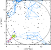 |
Fig. 1. Tetrahedra in a spherical cell: the empty circles represent the 3D distribution of CDM particles in a cubic region of size 8 h−1 Mpc projected in 2D. They represent the input set of points on which we perform the Delaunay tessellation. The gray circle represents the spherical cell. For clarity, we only show, in dashed light blue lines, the tetrahedra which have their four vertices included in a slice of 1.5 h−1 Mpc (in the z-direction) around the center of the cell. As an example we highlight one tetrahedron overlapping the boundary of the spherical cell (dark blue in the bottom left-hand corner). The red and green filled circles represent the randomly distributed points over the tetrahedron, the green ones represent those points lying inside the spherical cell and that are then used to assign a velocity to the corresponding region of the tetrahedron. This is repeated for all tetrahedrons of the tessellation that overlap the boundary of the spherical cell. |
Each Voronoi tetrahedron can be described by a set of four points x1, x2, x3 and x4 where xi = (xi, yi, zi); they are therefore defined by the transformation matrix (see Pueblas & Scoccimarro 2009)
 (1)
(1)
where Δxi = xi − x1. As a result, the volume of the j-th tetrahedron can be computed as wj = |Ψ|/6. The matrix Ψ can also be seen as the matrix transforming the basis of the vectors composed of Δx2, Δx3 and Δx4 into the cartesian basis. If the position s is taken as the tetrahedron basis, then the corresponding coordinates in the cartesian basis are obtained as x = x1 + Ψs. The same can be applied in order to interpolate linearly the velocity of a point located in s,
 (2)
(2)
where
 (3)
(3)
For tetrahedra entirely contained inside the sphere one can show that the volume average of the interpolated velocity field inside the tetrahedron is the arithmetic mean of the four velocities taken at each vertex;  . As mentioned above, for tetrahedra crossing the cell boundary, we randomly populate their volume with a uniform distribution of N = 100 points (see Fig. 1) and we evaluate their corresponding velocities using Eq. (2). The volume-averaged velocity assigned to the tetrahedron can be computed as
 (4)
(4)
where Nin is the number of random points belonging to the spherical cell and the fraction of its volume inside the spherical cell can be estimated as  . Finally, the volume-averaged velocity assigned to the spherical cell is obtained with the sum
 (5)
(5)
where Nt is the total number of tetrahedra with at least one vertex belonging to the spherical cell. We note that we checked explicitly that in the most clustered catalogue, that is, the one corresponding to the ΛCDM cosmology at z = 0, the number of objects in a spherical cell is always greater than 8, thus avoiding empty cells.
Once the velocity and density grids of 5123 regularly spaced sampling points have been built, we can Fourier transform them by means of a Fast Fourier Transform algorithm. Since a simple count-in-cell density interpolation can be severely affected by aliasing when transforming to Fourier space, we employ an interlacing technique to reduce this spurious contribution (Hockney & Eastwood 1988; Sefusatti et al. 2016). Regarding the shot noise correction, we neglect it because the mean number of particles in each cell is  which corresponds to a 3% contribution to the variance at z = 1.5 and for the Mν = 0.53eV (snapshot having the lowest variance). We then compute the divergence of the velocity field θk by simply combining the three velocity grids as θk = i(kxvx + kyvy + kzvz). Then the density power spectrum Pδδ, the cross power spectrum Pδθ, and the divergence of the velocity power spectrum Pθθ are estimated by averaging over spherical shells in k-space. We note that we also average the modes, and assign the value of the angular average of the spectra to the k-space position of the corresponding mode average.
4. Results
Our goal is to provide accurate prescriptions to estimate the Pθθ and Pδθ auto- and cross-spectra in the regime where the perturbative approach fails in describing the velocity field and its power spectra (Crocce et al. 2012).
The fitting functions for the velocity power spectra adopted in Jennings et al. (2011) and Jennings (2012) describe the nonlinear velocity spectra Pθθ and Pδθ in terms of the nonlinear matter power spectrum Pδδ assuming a cosmology-independent relation between these quantities at redshift zero and introducing a scaling relation to extend the results at higher redshift. However, the relations between Pθθ and Pδδ and between Pθδ and Pδδ are not universal and depend strongly, in the first place, on the amplitude of linear fluctuations, as measured for example by σ8. This is particularly evident when comparing our set of massive neutrino cosmologies where the neutrino mass directly affects this quantity. In Fig. 2, the velocity spectra (auto and cross) are plotted as a function of the corresponding matter density power spectrum. These relations, far from being universal, clearly depend as much on redshift as they depend on the sum of neutrino masses, via the amplitude suppression induced by the latter. The cosmology-independence of the fit proposed by Jennings et al. (2011) is perhaps justified by the fact that the different cosmological models considered in that paper share the same amplitude normalisation in terms of the σ8 parameter.
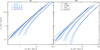 |
Fig. 2. Relation between the velocity cross (left panel) and auto (right panel) spectra with the density auto-spectrum for the different redshifts and cosmologies considered in this work. The shade of blue represents different values of the total neutrino mass, darker when the neutrino mass is increasing. The various redshifts (z = 0, 0.5, 1, 1.5) are respectively represented with dot-dashed, long dashed, short dashed, and solid lines. The black dotted line represents for each redshift the linear mapping ( |


We chose a different approach to fit the velocity power spectra measured in the DEMNUni-I simulations. In our set of simulations, all cosmological models considered present the same amplitude for the total-matter power spectrum in the large-scale limit, matching current CMB constraints (Planck Collaboration XIII 2016). However, since the presence of massive neutrinos suppresses the growth of fluctuations below the free-streaming scale, we obtain quite different values for σ8(z = 0) as a function of neutrino mass (see Table 1). We are thus able to test a wider range of amplitudes and shapes of the linear power spectrum, since neutrinos affect both of them.
Figure 3 shows the ratio of the measured power spectrum of the density, velocity, and cross to their respective linear predictions. Across all cosmological models and redshifts considered, we notice the usual increase in small-scale power for the density power spectrum Pδδ as well as the slower nonlinear growth for the velocity perturbations leading to a nonlinear suppression of Pδθ and particularly of Pθθ (see e.g., Bernardeau et al. 2002).
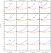 |
Fig. 3. Ratio between nonlinear (measured) PNL and the linear (predicted) PLin power spectra in the ΛCDM case (∑mν = 0) and for the three neutrino masses (∑mν = {0.17, 0.3, 0.53} eV). The density–density, density–velocity divergence, and velocity divergence–velocity divergence spectra are represented by blue solid, red short dashed, and green long dashed lines, respectively. Each row shows the redshift evolution of these ratios (from top to bottom panels: z = 0, 0.5, 1. and 1.5.) |
Following Hahn et al. (2015), we therefore choose to model the nonlinear corrections to the velocity spectra in terms of damping functions, in order to account for the suppression of power characterising the velocity divergence field. In addition, the level of such suppression will be, as observed, dependent on cosmology. In our approach, we do not assume a universal mapping independently of the considered cosmology. The main motivation supporting this is the empirical evidence that the velocity spectra are damped differently for different cosmological backgrounds.
In this section we explain our general fitting formulae and show how the chosen parameters depend on the value of the overall matter clustering. For simplicity, we first employ fitting functions featuring one single free parameter that accounts for the damping of the linear prediction in the nonlinear regime (see Fig. 3). As first approximation, one can model the velocity spectra using one single damping function such as
 (6)
(6)
and
 (7)
(7)
where the (only) two free parameters are the typical damping scales kδ and kθ. We note that  refers to the nonlinear density-density CDM power spectrum computed from the Halofit calibration of Takahashi et al. (2012) while
  refers to the linear auto-spectrum of the velocity divergence which can be computed as
  .
.
The fit for the velocity power spectra is carried out using a least-squares approach, that is, we compute the likelihood of the parameters given the measured spectra with the χ2 function defined as
![Mathematical equation: $$ \begin{aligned} \chi ^2=\sum _{i=1}^{N}\frac{\left[ P_{x{ y}}^\mathrm{NL}(k_i)-P_{x{ y}}(k_i) \right]^2}{\sigma _i^2}, \end{aligned} $$](/articles/aa/full_html/2019/02/aa34513-18/aa34513-18-eq18.gif) (8)
(8)
where N is the total number of wavenumbers considered in the fit,  is the measured auto- or cross-spectrum and
  is its variance at the i−th wave mode ki. We limit the fitting range to kmax = 0.6 h Mpc−1, and since we have only one realisation for each cosmology we neglect the shot-noise and the nonGaussian contributions to the covariance between wave modes. Under these assumptions the error can be approximated as
 (9)
(9)
We note that our choice of using a fixed power α = 1 for the exponent, rather than having more degrees of freedom (i.e., exp(−(k/k*)α)), comes from a further test we carried out, which shows that the best-fit value of α is always close to 1 if we treat it as a free parameter (see also Hahn et al. 2015). We note that this is at odds with what one would expect when considering the propagator in renormalized perturbation theory (Bernardeau et al. 2008, 2012; Crocce et al. 2012), in which case α would be closer to 2.
The results of the fit are shown in the first and third columns of Fig. 4. One can see that the simple modeling provided by Eq. (6) is able to reproduce the cross power spectrum Pδθ in the nonlinear regime with an accuracy better than 5% up to k = 0.65 h Mpc−1. The fit is not working as well for the auto spectrum Pθθ (third panel) especially at low redshift. The inaccuracy in this case can reach 7–8% in between k = 0.1 h Mpc−1 and k = 0.3 h Mpc−1. Nonetheless, this approximation could be considered sufficient for analyses that do not require precision around the BAO scale of better than few percent. For more general applications, we improve the accuracy of the model by increasing the degrees of freedom of the fitting functions.
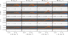 |
Fig. 4. Fractional deviation of the measured velocity spectra from our best-fitting models. Different rows mark different redshifts as specified on the left of the panels. The first and third columns show the fit of Pδθ using Eq. (6), and the fit of Pθθ using Eq. (7). The second and fourth columns show results corresponding to Eqs. (10) and (11). The black dashed line marks the 0, while the light/dark gray bands represent the 5%/3% deviations from the measurements. Finally, the red shaded color shows the results for various neutrino masses (darker when increasing the neutrino mass) using the fitted shape parameters while the blue shaded lines show the results when using the fitted dependance of the shape parameters with respect to σ8, m (see Eq. (12)). |
In the case of the cross-power spectrum, it is sufficient to add only one parameter b, which we fit between k = 0.55 and k = 0.7 h Mpc−1,
 (10)
(10)
For the auto-spectrum Pθθ, it turns out that two extra free parameters are required for a proper gain in accuracy. We therefore adopt a polynomial fitting for the damping function, as
 (11)
(11)
involving three parameters, which we fit in the range 0.01 < k < 0.7 h Mpc−1. The performances of the new fitting functions are shown in the second and fourth columns of Fig. 4. In this case, the measurements of Pθθ are reproduced with a maximum systematic error of 3% on all scales below k = 0.7 h Mpc−1, and for all redshifts and neutrino masses considered. We therefore use a total of only five free parameters kδ, b, a1, a2 and a3 to mimic, with a 3% level accuracy at k < 0.7 h Mpc−1, the nonlinear effects on both the auto- and cross-spectra Pθθ and Pδθ.
Let us now focus on the sensitivity of these parameters to cosmology and specifically to the overall amplitude of the matter power spectrum. From our set of four simulations at four different redshifts we are able to span a large range of possible values of σ8, which we use as a proxy for the amount of nonlinearities. Regarding neutrino cosmologies it is necessary to choose whether we use the σ8 defined for cold dark matter only, σ8, c, or the one defined for the total matter, σ8, m. It has been shown (Castorina et al. 2015) that regarding the bias or the nonlinear effects on the density power spectrum Pδδ, what matters is the amplitude of the cold dark matter clustering and not the total one. We have analyzed the dependency of the fitted parameters with respect to both amplitudes σ8, c and σ8, m and we found that one should use the total matter σ8, m parameter in order to assess the correct values of kδ, b, a1, a2 and a3; at least, this choice is the one that lowers the residual dependency with respect to the neutrino mass. Figure 5 shows that the cosmological dependance of the fitting parameters can be mostly encapsulated into the σ8, m parameter evaluated at the corresponding redshift. The most relevant example is the good match at redshift 1.5 of the ΛCDM simulation with the Mν = 0.53eV simulation at redshift 1; these simulations share almost the same value of the total matter σ8, m, while differing significantly in the power spectrum shape. For the two cases, we obtain the same values for the fitted parameters kδ and kθ.
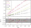 |
Fig. 5. Top panel: dependence of the fitting parameters kδ, b, kθ, a1, a2 and a3 on the total matter clustering amplitude σ8,m at each redshift, in the corresponding simulation (symbols). Lines are showing the fit of the dependance. Bottom panel: residual between the fitted σ8,m dependance and the measured one. |
On the contrary, when using the cold dark matter σ8,c parameter (see Table 1) the residuals are increasing because of spurious neutrino mass dependence when going from one cosmology to another. This effect can be explained by the fact that if massive neutrinos have a weak effect on the dark matter clustering in the nonlinear regime, they add, instead, a relevant contribution to the velocity field which is felt by dark matter particles. As a result, it seems that the preferred dependence on the total matter σ8,m comes from the fact that nonlinearities in the velocity field are generated by the whole matter distribution (cold dark matter plus neutrinos). This confirms the need for running cosmological simulations including massive neutrino particles in order to generate a velocity field correctly treated in the nonlinear regime, especially for what concerns RSD analyses.
The final step of our fitting process is to fit the dependence of the shape parameters kδ, b, a1, a2, a3 and kθ with respect to the total matter σ8,m. To this purpose we limit ourselves to linear or quadratic fitting depending on the parameters, finding
 (12)
(12)
where σ8,m refers to the linear rms of total matter fluctuations computed at the required redshift. Therefore, the cross- and auto-spectra Pδθ and Pθθ can be computed as follows: compute the linear and nonlinear cold dark matter power spectrum at the required redshift, evaluate the linear σ8,m as
 (13)
(13)
where R = 8h−1Mpc, ![Mathematical equation: $ \hat W(x)\equiv 3/x^3\left [ \sin x - x\cos x\right] $](/articles/aa/full_html/2019/02/aa34513-18/aa34513-18-eq26.gif) and Pm is the linear total matter power spectrum. Finally, compute the kδ, b, kθ, a1, a2 and a3 parameters from Eq. (12) and the velocity spectra from Eqs. (10) and (11) (or (6) and (7) depending on the required accuracy). In order to summarize the overall accuracy of our fitting formula, we show in Fig. 4 the comparison between the intrinsic accuracy of the fitting formula (for the shape) in red shade and the final accuracy obtained assuming the additional fitted dependency on σ8,m in blue shade. One can see that the accuracy below k = 0.8 h Mpc−1 is about 3% for the cross-power spectrum while the auto-power spectrum reaches a similar accuracy below k = 0.7 h Mpc−1.
and Pm is the linear total matter power spectrum. Finally, compute the kδ, b, kθ, a1, a2 and a3 parameters from Eq. (12) and the velocity spectra from Eqs. (10) and (11) (or (6) and (7) depending on the required accuracy). In order to summarize the overall accuracy of our fitting formula, we show in Fig. 4 the comparison between the intrinsic accuracy of the fitting formula (for the shape) in red shade and the final accuracy obtained assuming the additional fitted dependency on σ8,m in blue shade. One can see that the accuracy below k = 0.8 h Mpc−1 is about 3% for the cross-power spectrum while the auto-power spectrum reaches a similar accuracy below k = 0.7 h Mpc−1.
5. Summary
We set up an original algorithm in order to estimate the velocity field in cosmological N-body simulations. From those measurements performed on sixteen particle distributions spanning four different cosmological models and four redshifts, that is, a series of 16 snapshots, we have shown that the mapping from the nonlinear CDM density power spectrum Pδδ to the nonlinear velocity spectra Pδθ and Pθθ cannot be considered as universal but shows a clear dependence on the amplitude of dark matter clustering (see Fig. 2).
Adopting a very simple modeling involving only two free parameters, we managed to reproduce our measurements with a precision of 3% below k = 0.6 h Mpc−1 for the cross-power spectrum Pδθ. However, we reached only a 5% accuracy at redshifts higher than or equal to z = 0.5 and for k lower than 0.7 h Mpc−1. We then present an improved version of the fitting function which involves a total of five free parameters (two for the cross-spectrum and three for the auto-spectrum) and allows us to obtain an overall accuracy of 3% for wave modes lower than 0.7 h Mpc−1.
Finally, we we showed evidence of the dependence of the shape parameters of the proposed fitting functions on the total matter rms fluctuations in spheres of radius 8 h−1 Mpc and proposed simple fitting forms for the shape parameters with respect to the σ8,m parameter evaluated at the considered redshift. This preferred dependence with respect to the total matter amplitude rather than the cold dark matter one confirms the relevance of the neutrino perturbations on the cold dark matter velocity field in the nonlinear regime.
In a future paper we shall generalize these results using the second set of the DEMNUni cosmological simulations that include dynamical dark energy, extending our study of the dependence of the shape parameters on the rms amplitude of clustering σ8,m.
Acknowledgments
This work were developed in the framework of the ERC Darklight project, supported by an Advanced Research Grant of the European Research Council (n. 291521). CC, LG and ES also acknowledge a contribution from ASI through grant I/023/12/0. ES is also supported by INFN INDARK PD51 grant. The DEMNUni-I simulations were carried out in the framework of the “The Dark Energy and Massive-Neutrino Universe” using the Tier-0 IBM BG/Q Fermi machine of the Centro Interuniversitario del Nord-Est per il Calcolo Elettronico (CINECA). We acknowledge a generous CPU allocation by the Italian SuperComputing Resource Allocation (ISCRA).
References
- Ali-Haïmoud, Y., & Bird, S. 2013, MNRAS, 428, 3375 [NASA ADS] [CrossRef] [Google Scholar]
- Amendola, L., Appleby, S., Avgoustidis, A., et al. 2018, Liv. Rev. Rel., 21, 2 [Google Scholar]
- Baldi, M., Villaescusa-Navarro, F., Viel, M., et al. 2014, MNRAS, 440, 75 [NASA ADS] [CrossRef] [Google Scholar]
- Bassett, B., & Hlozek, R. 2010, in Baryon acoustic oscillations, ed. P. Ruiz-Lapuente, 246 [Google Scholar]
- Bernardeau, F., & van de Weygaert, R. 1996, MNRAS, 279, 693 [NASA ADS] [CrossRef] [Google Scholar]
- Bernardeau, F., van de Weygaert, R., Hivon, E., & Bouchet, F. R. 1997a, MNRAS, 290, 566 [NASA ADS] [CrossRef] [Google Scholar]
- Bernardeau, F., van de Weygaert, R., Hivon, E., & Bouchet, F. R. 1997b, MNRAS, 290, 566 [NASA ADS] [CrossRef] [Google Scholar]
- Bernardeau, F., Colombi, S., Gaztañaga, E., & Scoccimarro, R. 2002, Phys. Rev., 367, 1 [Google Scholar]
- Bernardeau, F., Crocce, M., & Scoccimarro, R. 2008, Phys. Rev. D, 78, 103521 [NASA ADS] [CrossRef] [Google Scholar]
- Bernardeau, F., Crocce, M., & Scoccimarro, R. 2012, Phys. Rev. D, 85, 123519 [NASA ADS] [CrossRef] [Google Scholar]
- Bianchi, D., Percival, W. J., & Bel, J. 2016, MNRAS, 463, 3783 [NASA ADS] [CrossRef] [Google Scholar]
- Bose, B., & Koyama, K. 2016, J. Cosmol. Astropart. Phys., 8, 032 [NASA ADS] [CrossRef] [Google Scholar]
- Carbone, C., Petkova, M., & Dolag, K. 2016, J. Cosmol. Astropart. Phys., 7, 034 [NASA ADS] [CrossRef] [Google Scholar]
- Castorina, E., Sefusatti, E., Sheth, R. K., Villaescusa-Navarro, F., & Viel, M. 2014, J. Cosmol. Astropart. Phys., 2, 49 [NASA ADS] [CrossRef] [Google Scholar]
- Castorina, E., Carbone, C., Bel, J., Sefusatti, E., & Dolag, K. 2015, J. Cosmol. Astropart. Phys., 7, 043 [Google Scholar]
- Crocce, M., Scoccimarro, R., & Bernardeau, F. 2012, MNRAS, 427, 2537 [NASA ADS] [CrossRef] [Google Scholar]
- Emberson, J. D., Yu, H.-R., Inman, D., et al. 2017, Res. Astron. Astrophys., 17, 085 [NASA ADS] [CrossRef] [Google Scholar]
- Fonseca de la Bella, L., Regan, D., Seery, D., & Hotchkiss, S. 2017, J. Cosmol. Astropart. Phys., 11, 039 [NASA ADS] [CrossRef] [Google Scholar]
- Guzzo, L., Pierleoni, M., Meneux, B., et al. 2008, Nature, 451, 541 [NASA ADS] [CrossRef] [PubMed] [Google Scholar]
- Hahn, O., Angulo, R. E., & Abel, T. 2015, MNRAS, 454, 3920 [NASA ADS] [CrossRef] [Google Scholar]
- Hand, N., Seljak, U., Beutler, F., & Vlah, Z. 2017, J. Cosmol. Astropart. Phys., 10, 009 [NASA ADS] [CrossRef] [Google Scholar]
- Hashimoto, I., Rasera, Y., & Taruya, A. 2017, Phys. Rev. D, 96, 043526 [NASA ADS] [CrossRef] [Google Scholar]
- Hockney, R. W., & Eastwood, J. W. 1988, Computer Simulation using Particles (New York: Taylor & Francis) [Google Scholar]
- Inman, D., Emberson, J. D., Pen, U.-L., et al. 2015, Phys. Rev. D, 92, 023502 [NASA ADS] [CrossRef] [Google Scholar]
- Jennings, E. 2012, MNRAS, 427, L25 [NASA ADS] [Google Scholar]
- Jennings, E., Baugh, C. M., & Pascoli, S. 2011, MNRAS, 410, 2081 [NASA ADS] [Google Scholar]
- Jennings, E., Baugh, C. M., & Hatt, D. 2015, MNRAS, 446, 793 [NASA ADS] [CrossRef] [Google Scholar]
- Kaiser, N. 1987, MNRAS, 227, 1 [NASA ADS] [CrossRef] [Google Scholar]
- Koda, J., Blake, C., Davis, T., et al. 2014, MNRAS, 445, 4267 [NASA ADS] [CrossRef] [Google Scholar]
- Lesgourgues, J., & Pastor, S. 2006, Phys. Rev., 429, 307 [Google Scholar]
- Liu, J., Bird, S., Zorrilla Matilla, J. M., et al. 2018, J. Cosmol. Astropart. Phys., 3, 049 [Google Scholar]
- Matsubara, T. 2008a, Phys. Rev. D, 78, 083519 [NASA ADS] [CrossRef] [Google Scholar]
- Matsubara, T. 2008b, Phys. Rev. D, 77, 063530 [NASA ADS] [CrossRef] [Google Scholar]
- Okumura, T., Hand, N., Seljak, U., Vlah, Z., & Desjacques, V. 2015, Phys. Rev. D, 92, 103516 [NASA ADS] [CrossRef] [Google Scholar]
- Palanque-Delabrouille, N., Yèche, C., Baur, J., et al. 2015, J. Cosmol. Astropart. Phys., 11, 011 [CrossRef] [Google Scholar]
- Perko, A., Senatore, L., Jennings, E., & Wechsler, R. H. 2016, ArXiv e-prints [arXiv:1610.09321] [Google Scholar]
- Pezzotta, A., de la Torre, S., Bel, J., et al. 2017, A&A, 604, A33 [NASA ADS] [CrossRef] [EDP Sciences] [Google Scholar]
- Planck Collaboration XIII. 2016, A&A, 594, A13 [NASA ADS] [CrossRef] [EDP Sciences] [Google Scholar]
- Pueblas, S., & Scoccimarro, R. 2009, Phys. Rev. D, 80, 043504 [NASA ADS] [CrossRef] [Google Scholar]
- Reid, B. A., & White, M. 2011, MNRAS, 417, 1913 [NASA ADS] [CrossRef] [Google Scholar]
- Romano-Díaz, E., & van de Weygaert, R. 2007, MNRAS, 382, 2 [NASA ADS] [CrossRef] [Google Scholar]
- Sánchez, A. G., Scoccimarro, R., Crocce, M., et al. 2017, MNRAS, 464, 1640 [NASA ADS] [CrossRef] [Google Scholar]
- Sato, M., & Matsubara, T. 2011, Phys. Rev. D, 84, 043501 [NASA ADS] [CrossRef] [Google Scholar]
- Scoccimarro, R. 2004, Phys. Rev. D, 70, 083007 [NASA ADS] [CrossRef] [Google Scholar]
- Sefusatti, E., Crocce, M., Scoccimarro, R., & Couchman, H. M. P. 2016, MNRAS, 460, 3624 [NASA ADS] [CrossRef] [Google Scholar]
- Seljak, U., & McDonald, P. 2011, J. Cosmol. Astropart. Phys., 11, 039 [NASA ADS] [CrossRef] [Google Scholar]
- Senatore, L., & Zaldarriaga, M. 2014, ArXiv e-prints [arXiv:1409.1225] [Google Scholar]
- Takahashi, R., Sato, M., Nishimichi, T., Taruya, A., & Oguri, M. 2012, ApJ, 761, 152 [NASA ADS] [CrossRef] [Google Scholar]
- Taruya, A., Nishimichi, T., Saito, S., & Hiramatsu, T. 2009, Phys. Rev. D, 80, 123503 [NASA ADS] [CrossRef] [Google Scholar]
- Taruya, A., Nishimichi, T., & Saito, S. 2010, Phys. Rev. D, 82, 063522 [NASA ADS] [CrossRef] [Google Scholar]
- Taruya, A., Nishimichi, T., & Bernardeau, F. 2013, Phys. Rev. D, 87, 083509 [NASA ADS] [CrossRef] [Google Scholar]
- Uhlemann, C., Kopp, M., & Haugg, T. 2015, Phys. Rev. D, 92, 063004 [NASA ADS] [CrossRef] [Google Scholar]
- Upadhye, A., Kwan, J., Pope, A., et al. 2016, Phys. Rev. D, 93, 063515 [NASA ADS] [CrossRef] [Google Scholar]
- Valageas, P. 2011, A&A, 526, A67 [NASA ADS] [CrossRef] [EDP Sciences] [Google Scholar]
- van de Weygaert, R., & Bernardeau, F. 1998, in Large Scale Structure: Tracks and Traces, eds. V. Mueller, S. Gottloeber, J. P. Muecket, & J. Wambsganss, 207 [Google Scholar]
- Viel, M., Haehnelt, M. G., & Springel, V. 2010, J. Cosmol. Astropart. Phys., 6, 015 [NASA ADS] [CrossRef] [Google Scholar]
- Villaescusa-Navarro, F., Marulli, F., Viel, M., et al. 2014, J. Cosmol. Astropart. Phys., 3, 11 [NASA ADS] [CrossRef] [Google Scholar]
- Villaescusa-Navarro, F., Banerjee, A., Dalal, N., et al. 2018, ApJ, 861, 53 [NASA ADS] [CrossRef] [Google Scholar]
- Vlah, Z., Castorina, E., & White, M. 2016, J. Cosmol. Astropart. Phys., 12, 007 [NASA ADS] [CrossRef] [Google Scholar]
- Weinberg, D. H., Mortonson, M. J., Eisenstein, D. J., et al. 2013, Phys. Rev., 530, 87 [Google Scholar]
- Yu, Y., Zhang, J., Jing, Y., & Zhang, P. 2015, Phys. Rev. D, 92, 083527 [NASA ADS] [CrossRef] [Google Scholar]
- Zel’dovich, Y. B. 1970, A&A, 5, 84 [NASA ADS] [Google Scholar]
- Zennaro, M., Bel, J., Villaescusa-Navarro, F., et al. 2017, MNRAS, 466, 3244 [NASA ADS] [CrossRef] [Google Scholar]
- Zhang, P., Pan, J., & Zheng, Y. 2013, Phys. Rev. D, 87, 063526 [NASA ADS] [CrossRef] [Google Scholar]
- Zhang, P., Zheng, Y., & Jing, Y. 2015, Phys. Rev. D, 91, 043522 [NASA ADS] [CrossRef] [Google Scholar]
- Zheng, Y., Zhang, P., Jing, Y., Lin, W., & Pan, J. 2013, Phys. Rev. D, 88, 103510 [NASA ADS] [CrossRef] [Google Scholar]
- Zheng, Y., Zhang, P., & Jing, Y. 2015, Phys. Rev. D, 91, 043523 [NASA ADS] [CrossRef] [Google Scholar]
All Tables
Parameters of the four νΛCDM simulations that change among the different realisations.
All Figures
|
Fig. 1. Tetrahedra in a spherical cell: the empty circles represent the 3D distribution of CDM particles in a cubic region of size 8 h−1 Mpc projected in 2D. They represent the input set of points on which we perform the Delaunay tessellation. The gray circle represents the spherical cell. For clarity, we only show, in dashed light blue lines, the tetrahedra which have their four vertices included in a slice of 1.5 h−1 Mpc (in the z-direction) around the center of the cell. As an example we highlight one tetrahedron overlapping the boundary of the spherical cell (dark blue in the bottom left-hand corner). The red and green filled circles represent the randomly distributed points over the tetrahedron, the green ones represent those points lying inside the spherical cell and that are then used to assign a velocity to the corresponding region of the tetrahedron. This is repeated for all tetrahedrons of the tessellation that overlap the boundary of the spherical cell. |
| In the text | |
|
Fig. 2. Relation between the velocity cross (left panel) and auto (right panel) spectra with the density auto-spectrum for the different redshifts and cosmologies considered in this work. The shade of blue represents different values of the total neutrino mass, darker when the neutrino mass is increasing. The various redshifts (z = 0, 0.5, 1, 1.5) are respectively represented with dot-dashed, long dashed, short dashed, and solid lines. The black dotted line represents for each redshift the linear mapping ( |
| In the text | |
|
Fig. 3. Ratio between nonlinear (measured) PNL and the linear (predicted) PLin power spectra in the ΛCDM case (∑mν = 0) and for the three neutrino masses (∑mν = {0.17, 0.3, 0.53} eV). The density–density, density–velocity divergence, and velocity divergence–velocity divergence spectra are represented by blue solid, red short dashed, and green long dashed lines, respectively. Each row shows the redshift evolution of these ratios (from top to bottom panels: z = 0, 0.5, 1. and 1.5.) |
| In the text | |
|
Fig. 4. Fractional deviation of the measured velocity spectra from our best-fitting models. Different rows mark different redshifts as specified on the left of the panels. The first and third columns show the fit of Pδθ using Eq. (6), and the fit of Pθθ using Eq. (7). The second and fourth columns show results corresponding to Eqs. (10) and (11). The black dashed line marks the 0, while the light/dark gray bands represent the 5%/3% deviations from the measurements. Finally, the red shaded color shows the results for various neutrino masses (darker when increasing the neutrino mass) using the fitted shape parameters while the blue shaded lines show the results when using the fitted dependance of the shape parameters with respect to σ8, m (see Eq. (12)). |
| In the text | |
|
Fig. 5. Top panel: dependence of the fitting parameters kδ, b, kθ, a1, a2 and a3 on the total matter clustering amplitude σ8,m at each redshift, in the corresponding simulation (symbols). Lines are showing the fit of the dependance. Bottom panel: residual between the fitted σ8,m dependance and the measured one. |
| In the text | |
Current usage metrics show cumulative count of Article Views (full-text article views including HTML views, PDF and ePub downloads, according to the available data) and Abstracts Views on Vision4Press platform.
Data correspond to usage on the plateform after 2015. The current usage metrics is available 48-96 hours after online publication and is updated daily on week days.
Initial download of the metrics may take a while.